Effective photon-photon interaction in a
two-dimensional “photon fluid”

Abstract

We formulate an effective theory for the atom-mediated photon-photon interactions in a two-dimensional “photon fluid” confined in a Fabry-Perot resonator. With the atoms modelled by a collection of anharmonic Lorentz oscillators, the effective interaction is evaluated to second order in the coupling constant (the anharmonicity parameter). The interaction has the form of a renormalized two-dimensional delta-function potential, with the renormalization scale determined by the physical parameters of the system, such as density of atoms and the detuning of the photons relative to the resonance frequency of the atoms. For realistic values of the parameters, the perturbation series has to be resummed, and the effective interaction becomes independent of the “bare” strength of the anharmonic term. The resulting expression for the non-linear Kerr susceptibility, is parametrically equal to the one found earlier for a dilute gas of two-level atoms. Using our result for the effective interaction parameter, we derive conditions for the formation of a photon fluid, both for Rydberg atoms in a microwave cavity and for alkali atoms in an optical cavity.

I Introduction

Quantum physics in two-dimensions has many interesting features which give rise to effects that cannot be seen in three-dimensional systems. One of the most interesting two-dimensional effects is the formation of incompressible electron fluids that characterize the plateau states of the quantum Hall effect Girvin90 . Also high temperature superconductivity is believed to be essentially a two-dimensional effect.

The interest in the physics of low-dimensional systems has motivated both theoretical and experimental searches for new kinds of two-dimensional many-body systems. In the case of weakly interacting Bose-condensed atomic gases, two-dimensionality can be reached in highly asymmetric traps asymmetric , and quantum states similar to the quantum Hall states have been predicted for such systems when in rapid rotation BEC .

Another idea that has been advocated by one of us chiao1 ; Chiao2000 is that photons also, under specific conditions in photonic traps, can form a two-dimensional system of weakly interacting particles with an effective mass determined by the (fixed) momentum in the suppressed dimension. Such a photon gas can in principle undergo phase transitions, much like a cold atomic gas, and can in a condensed phase sustain vortices and sound excitations, in a manner similar to that of an ordinary superfluid.

This picture of the photons as a two-dimensional fluid has been based on the (effective) Maxwell theory of electromagnetic waves in a non-linear medium where only one longitudinal mode inside a cavity is excited by an incoming laser beam. The corresponding mean field equation has the same form as the Gross-Pitaevski equation, or the non-linear Schrödinger equation with a quartic non-linearity, and when coupled to an external driving field it has been referred to as the Luigiato-Lefever (LL) equation. The LL equation has been used to discuss the apparence of transverse patterns in the light trapped inside Fabry-Perot and ring cavities Lugiato87 .

The LL equation is a non-linear classical field equation, but it can also be interpreted as a quantum field theory with the electromagnetic field as an operator field. The non-linear term is then viewed as a short range ($\delta$-function) photon-photon interaction. This interpretation is the basis for the photon fluid idea, and it has implications beyond the classical non-linear optics description.

However, the interpretation of the non-linear field equation as a quantum theory raises several questions. One has to do with the dimensional reduction itself. When only the fundamental longitudinal mode is excited there is clearly an effective reduction of dimension, since the dynamics is restricted to the two transverse directions. This corresponds to the situation where the cavity is small, with a length in the longitudinal direction of the order of half a wave length. In the optical regime such a resonator is extremely small, and even if it can be made in principle, a simpler realization of a small resonator is in the microwave regime in conjunction with Rydberg atoms which can couple strongly to the microwave photons. For the cavities that are presently used in laser experiments the longitudinal mode is highly excited relative to the fundamental mode, and in this case two-dimensionality is obtained only as long as the scattering to other longitudinal modes can be neglected.

Another question concerns the photon-photon scattering chiao2 . A two-dimensional delta-function interaction is only well defined to lowest order in perturbation theory, and in a full quantum description such a short range interaction is meaningful only as a renormalized interaction. This implies that the scattering amplitude is determined by a renormalization length in addition to the interaction strength. In the effective photon theory this is not a free parameter, but should be determined by the full microscopic theory of the photons interacting with the atoms of the non-linear medium.

In this work we will address the first question simply by assuming that only one longitudinal mode is excited. Our main objective will then be to examine the photon-photon interaction from a microscopic point of view. Of particular interest is to examine in what sense the effective interaction can be interpreted as a delta function interaction and to determine how the renormalized strength of the interaction depends on the physical parameters of the system.

The approach we will take is to derive the effective photon theory from from the full quantum theory of the electromagnetic field and the non-linear medium, rather than from a macroscopic description of the electromagnetic field. However, we will use the simplified model of the atoms in the medium as a collection of Lorentz oscillators supplemented by a quartic oscillator term to account for the non-linearity Boyd . At the quantum level, the linear Lorentz oscillator model yields “polaritons” as the coupled atom-photon degrees of freedom, as shown by Hopfield and others Hopfield58 ; Huttner92 .

In the next section (2) we use the Feynman path-integral method to find an expression for the interaction between the physical modes of the coupled photon-oscillator system in terms of an effective photon action. In Section 3 we consider the effective theory for the low-lying transverse momentum modes in a cavity where only the lowest longitudinal mode is excited, and derive the corresponding two-dimensional low-energy effective action. In the following section (4), we summarize the question of how to correctly describe the renormalized delta function interaction in two dimensions. Then in Section 5, we relate this to an evaluation of quantum corrections to the effective interaction (to second order in the coupling parameter) and determine the leading logarithmic corrections to the scattering amplitude. In Section 6 we summarize the physical scales and discuss the conditions under which interesting quantum phenomena like Bose-Einstein condensation and the formation of two-photon bound states may take place. In section 7 we examine two possible scenarios for experimental realizations of a 2D photon fluid. Based on order of magnitude estimates, we discuss under what conditions a photon fluid in thermal equilibrium may form for millimeter-wave photons interacting with Rydberg atoms and for optical photons interacting with alkali atoms. Both cases might offer possibilities to observe genuine quantum effects in an interacting photon gas, although our estimates indicate severe constraints on the physical parameters. We close this section by discussing a third possible scenario, in which a 2D photon fluid forms just inside the surface of a high-Q microsphere of glass. Concluding remarks are found in Section 8.

II 2 The effective photon action

For photons interacting off resonance with the atoms (i.e., the oscillators), the atoms have two types of effects on the scattered photons. There is a linear effect, where the elastic scattering off the atoms changes the dispersion of the photons. For photons with low transverse momentum in the cavity, this leads to a renormalization of the effective mass of the photons, which without the atoms is determined by the (fixed) longitudinal photon momentum $\hbar k_{L}$, as $m_{0}=\hbar k_{L}/c$. The other effect is the non-linear or anharmonic effect of the photon-atom interaction, which gives rise to the effective photon-photon interaction.

There are several ways to derive the effective photon action from the full quantum theory of photons and oscillators, all based on the assumption that the non-linear term is small and can be treated as a perturbation. One way is to solve, as the first step, the linear part of the problem exactly by diagonalizing the Hamiltonian. As the next step the non-linear terms can be expressed in terms of the transformed, decoupled variables; in this way the resonance problems, which would appear in a more direct perturbative treatment, are avoided. However, another simpler approach which we will adopt here, is to derive the effective action of the electromagnetic field by use of the Feynman path integral method, where a (non-local) field transformation yields the result without any matrix diagonalization. To check the result of this method we have also performed, in Appendix A, a decoupling of the linear variables by matrix diagonalization, and show that this can be done in a way that is substantially simpler than the standard method.

In this section we do not impose the cavity boundary conditions, which later will be used as constraints on the effective photon modes in order to derive a dimensionally reduced theory.

We start from the total classical action

$$\mbox{$$}{\cal S}[\vec{A},\vec{R}_{i}]={\cal S}_{\gamma}[\vec{A}]+{\cal S}_{M}[\vec{R}_{i}]+{\cal S}_{I}[\vec{A},\vec{R}_{i}]$$ (1)

which is the sum of a free photon part ${\cal S}_{\gamma}$, a matter part ${\cal S}_{M}$, for the atoms, and an interaction ${\cal S}_{I}$ which describes the their coupling to the radiation. $\vec{R}_{i}$ describes the atomic degrees of freedom, which here are given as the displacement vectors of a discrete set of oscillators labeled by $i$. In the following we will put $\hbar=c=1$.

The free photon part, ${\cal S}_{\gamma}$, is given by the Maxwell term

$$\mbox{$$}{\cal S}_{\gamma}=\frac{1}{2}\int d^{3}r\,dt\,[E^{2}-B^{2}]\text{ ,}$$ (2)

where $\vec{E}=-\dot{\vec{A}}$ and $\vec{B}=\nabla\times\vec{A}$ with $\vec{A}$ satisfying the Coulomb gauge condition $\nabla\cdot\vec{A}=0$. The oscillator part includes an anharmonic term,

$$\mbox{$$}{\cal S}_{M}=\int dt\,\sum_{i}\left(\frac{M}{2}{\dot{\vec{R}_{i}}}^{2}-\frac{M}{2}\omega_{0}^{2}{\vec{R}_{i}}^{2}-\frac{\Lambda M^{2}}{4}{\vec{R}_{i}}^{4}\right)\,,$$ (3)

and the atoms are coupled to the electromagnetic field via a dipole interaction,

$$\mbox{$$}{\cal S}_{I}=\int\,dt\sum_{i}q\vec{A}(\vec{r}_{i})\cdot\dot{\vec{R}_{i}}\,.$$ (4)

Here $\vec{r}_{i}$ is the spatial position of the i:th oscillator, and we shall furthermore assume that the atoms are uniformly distributed in space with a number density $\rho$, so that discrete sums can be replaced by integrals over a continuous position vector $\vec{r}$. Since only the transverse part of $\vec{R}$ couples to the photon field, it is consistent to neglect the longitudinal part and impose a Coulomb “gauge” condition also on the oscillator, i.e., $\nabla\cdot\vec{R}=0$.

The effective photon action ${\cal S}_{eff}[\vec{A}]$ is defined by the following (path) integral over the oscillator variables $R_{i}$

$$\mbox{$$}e^{i{\cal S}_{eff}[\vec{A}]}=\int\prod_{i}{\cal D}R_{i}\,e^{i{\cal S}[\vec{A},\vec{R}_{i}]}\,.$$ (5)

To perform the $R_{i}$ integrations, we go to Fourier space and expand to lowest order in $\Lambda$,

$$\mbox{$$}e^{i{\cal S}_{eff}} = e^{i{\cal S}_{\gamma}}\int\prod_{i}{\cal D}R_{i}\,e^{i\int\frac{d\omega}{2\pi}\sum_{i}[\frac{M}{2}\vec{R}_{i}(-\omega)(\omega^{2}-\omega_{0}^{2})\vec{R}_{i}(\omega)-i\omega q\vec{A}_{i}(-\omega)\cdot\vec{R}_{i}(\omega)]}$$

$$[ 1-\frac{i\Lambda M^{2}}{4}\int\prod_{n=1}^{4}\frac{d\omega_{n}}{2\pi}\,2\pi\delta(\sum_{n=1}^{4}\omega_{n})\vec{R}_{i}(\omega_{1})\cdot\vec{R}_{i}(\omega_{2})\vec{R}_{i}(\omega_{3})\cdot\vec{R}_{i}(\omega_{4})+O(\Lambda^{2})]\,.$$

The first term is evaluated directly by completing the square and making the shift
$\vec{R}_{i}(\omega)\rightarrow\vec{R}_{i}(\omega)-i\omega\frac{q}{M}\vec{A}_{i}{\cal D}_{0}(\omega)$, with ${\cal D}_{0}(\omega)$ as the retarded propagator,

$$\mbox{$$}{\cal D}_{0}(\omega)=\frac{1}{\omega^{2}-\omega_{0}^{2}+i\omega\epsilon}\,.$$ (7)

It yields the quadratic part of the effective action,

$$\mbox{$$}{\cal S}_{eff}^{(2)} = \frac{1}{2}\int d^{3}x\int\frac{d\omega}{2\pi}\,\vec{A}(\vec{x},-\omega)\left[\omega^{2}+\nabla^{2}-\eta^{2}\omega^{2}{\cal D}_{0}(\omega)\right]\vec{A}(\vec{x},\omega)\text{,}$$ (8)

where in this expression we have taken the continuum limit $\sum_{i}\rightarrow\rho\int d^{3}x$ and also introduced the effective plasma frequency $\eta=(\rho q^{2}/M)^{1/2}$.

The quartic $\vec{R}$ term in (II) is most easily evaluated by again performing the shift in $\vec{R}_{i}(\omega)$, to give $\vec{A}$ dependent terms of the form $\vec{A}^{4}$, $(\vec{A}\cdot\vec{A})(\vec{R}\cdot\vec{R}$) and $(\vec{A}\cdot\vec{R})(\vec{A}\cdot\vec{R})$. The $\vec{A}^{4}$ term can be directly re-exponentiated and gives a quartic contribution to the effective action, which in the continuum limit is

$$\mbox{$$}{\cal S}_{eff}^{(4)}=-\frac{2\pi\eta^{4}\Lambda}{4\rho}\int d^{3}x\int\prod_{n=1}^{4}\left[\frac{d\omega_{n}}{2\pi}\omega_{n}\,{\cal D}_{0}(\omega_{n})\right]\delta(\sum_{n=1}^{4}\omega_{n})\vec{A}(\omega_{1},\vec{x})\cdot\vec{A}(\omega_{2},\vec{x})\,\vec{A}(\omega_{3},\vec{x})\cdot\vec{A}(\omega_{4},\vec{x})\,.$$ (9)

The terms proportional to $(\vec{A}\cdot\vec{A})(\vec{R}\cdot\vec{R}$) and $(\vec{A}\cdot\vec{R})(\vec{A}\cdot\vec{R})$ can be evaluated using the formula,

$$\mbox{$$}\int\prod_{i}{\cal D}R_{i}\,e^{i\int\frac{d\omega}{2\pi}\sum_{i}[\frac{M}{2}\vec{R}_{i}(-\omega)(\omega^{2}-\omega_{0}^{2})\vec{R}_{i}(\omega)}R_{j}^{a}(\omega_{1})R_{k}^{b}(\omega_{2})={\cal N}\frac{2\pi i}{M}{\cal D}_{0}(\omega_{1})\delta(\omega_{1}+\omega_{2})\delta_{ab}\delta_{jk}\,\,\,,$$ (10)

where ${\cal N}$ is a field-independent normalization factor. They give, in principle, a correction term to the quadratic action, but due to the integration over ${\cal D}_{0}(\omega_{1})$ this correction term vanishes.

Note that the expansion and re-exponentiation of the non-linear term will generate correction terms, but these are higher order in $\Lambda$ and will be neglected. Thus, to first order in $\Lambda$, the effective action is given by the quadratic part (8) and the quartic term (9).

The effective action defined by (8) and (9) corresponds to a Lagrangian that is non-local in time. However by a further transformation it can be brought into a local form. We first note that the quadratic part of the action defines a modified dispersion equation

$$\mbox{$$}\omega^{2}-k^{2}-\eta^{2}\frac{\omega^{2}}{\omega^{2}-\omega_{0}^{2}}=0$$ (11)

with solutions

$$\mbox{$$}\omega_{\pm}^{2}(k^{2})=\frac{1}{2}\left(k^{2}+\omega_{0}^{2}+\eta^{2}\right)\pm\frac{1}{2}\sqrt{\left(k^{2}+\omega_{0}^{2}+\eta^{2}\right)^{2}-4\omega_{0}^{2}k^{2}}\,.$$ (12)

This equation defines the dispersion of the “polaritons”, i.e., the two decoupled degrees of freedom of the linear problem which mixes the photon and dipole variables. For $k^{2}<\omega_{0}^{2}+\eta^{2}$ $\omega_{-}$ represents essentially the photon mode and $\omega_{+}$ the dipole mode, whereas for $k^{2}>\omega_{0}^{2}+\eta^{2}$ the interpretation of the two modes is reversed. In the intermediate interval with $k^{2}\approx\omega_{0}^{2}$ the photon and the dipole modes are strongly mixed.

The following field transformation is now applied

$$\mbox{$$}\vec{A}(\vec{k},\omega)\rightarrow\vec{A}^{(\pm)}(\vec{k},\omega)=\sqrt{\frac{\omega^{2}-\vec{k}^{2}-\eta^{2}\frac{\omega^{2}}{\omega^{2}-\omega_{0}^{2}}}{\omega^{2}-\omega_{\pm}(k^{2})}}\;\;\vec{A}(\vec{k},\omega)$$ (13)

and this gives for the quadratic part of the action

$$\mbox{$$}S^{(2)}_{eff}=\frac{1}{2}\int\frac{d^{3}k}{(2\pi)^{3}}\int\frac{d\omega}{2\pi}\;\vec{A}^{(\pm)}(\vec{k},\omega)^{*}\;(\omega^{2}-\omega_{\pm}^{2})\;\vec{A}^{(\pm)}(\vec{k},\omega)\,.$$ (14)

The dependence on $\omega^{2}$ shows that the transformed action corresponds to a Lagrangian that is local in time. The non-locality in time has been traded for a non-locality in space, but this is less problematic in a Lagrangian formulation. Note, however, the ambiguity in the transformations (13), depending of which one of the solutions $\omega_{\pm}$ we choose. Clearly, the relevant choice is the one which fits the energy of the photons in the effective theory. This means $\omega_{-}$ for the case of red detuning (energy below $\omega_{0}$) and $\omega_{+}$ for blue detuning (energy above $\omega_{0}$).

When the transformed field is introduced in the quartic part of the effective action we make a further simplification by assuming that the fields satisfy the dispersion equation of the linear problem. This allows the following substitution

$$\mbox{$$}i\omega{\cal D}_{0}(\omega)\vec{A}(\vec{k},\omega) \rightarrow\lim_{\omega^{2}\rightarrow\omega_{\pm}^{2}}\ \frac{1}{\omega^{2}-\omega_{0}^{2}}\sqrt{\frac{\omega^{2}-\omega_{\pm}^{2}}{\omega^{2}-k^{2}-\eta^{2}\frac{\omega_{0}^{2}}{\omega^{2}-\omega_{0}^{2}}}}\;{\vec{E}}^{(\pm)}(\vec{k},\omega)$$ (15)

$$=\frac{1}{\sqrt{(\omega_{\pm}^{2}-\omega_{0}^{2})^{2}+\eta^{2}\omega_{0}^{2}}}\;{\vec{E}}^{(\pm)}(\vec{k},\omega)\,,$$

where ${\vec{E}}^{(\pm)}(\vec{k},\omega)=i\omega_{\pm}\vec{A}^{(\pm)}(\vec{k},\omega)$. For the interaction part of the action this gives the following expression,

$$\mbox{$$}{\cal S}_{eff}^{(4)} =-\frac{(2\pi)^{4}\eta^{4}\Lambda}{4\rho}\prod_{n=1}^{4}\left[\int\frac{d^{3}k_{n}\;d\omega_{n}}{(2\pi)^{4}}\frac{1}{\sqrt{(\omega_{\pm}(k_{n})^{2}-\omega_{0}^{2})^{2}+\eta^{2}\omega_{0}^{2}}}\right]\delta(\sum_{n=1}^{4}\vec{k}_{n})\delta(\sum_{n=1}^{4}\omega_{n})$$ (16)

$$\times\vec{E}^{(\pm)}(\vec{k}_{1},\omega_{1})\cdot\vec{E}^{(\pm)}(\vec{k}_{2},\omega_{2})\,\vec{E}^{(\pm)}(\vec{k}_{3},\omega_{3})\cdot\vec{E}^{(\pm)}(\vec{k}_{4},\omega_{4})\,.$$

The application of the dispersion equation to the field variables of the interaction term can be justified when this term is used perturbatively, with the fields satisfying the field equation of the unperturbed system. However, it is interesting to note that the expression (16) in fact is valid beyond this approximation, as is demonstrated by the diagonalization of the quadratic problem performed in Appendix A.

III 3 Dimensional reduction and the effective 2d $\phi^{4}$ theory

Due to the boundary conditions imposed by the mirrors, the component of the photon momentum normal to the mirrors (the longitudinal momentum) is quantized at discrete values. We assume an idealized situation with infinite flat mirrors, thus the longitudinal momenta are quantized as $k_{L}=\pi n/L$, with $L$ as the distance between the mirrors and $n$ as an integer. We also assume photons to be fed to the cavity by a laser (or maser) tuned close to resonance with one of the modes, either slightly below (red detuning), or slightly above the resonance (blue detuning). However, we do not take the effect of photons entering or departing the cavity explicitly into account, and in this sense we consider an idealized situation with perfectly reflecting mirrors. All the photons inside the cavity are assumed to be trapped in the same longitudinal mode, and throughout the paper we will assume this to be the lowest mode $n=1$.

The transverse components of the photon momentum $\vec{k}$ we assume to be restricted to small values, $k_{T}<<k_{L}$. The dispersion of free (non-interacting) photons inside the Fabry-Perot resonator becomes essentially that of 2D massive, non-relativistic particles chiao1 ,

$$\mbox{$$}\omega_{k}=\sqrt{k_{T}^{2}+k_{L}^{2}}\approx k_{L}+\frac{k_{T}^{2}}{2k_{L}},$$ (17)

with the longitudinal momentum $k_{L}$ playing the role of the photon mass. The dimensional reduction is then based on the assumption that only one longitudinal mode (the lowest) is excited, and that scattering to other modes can be neglected. We should stress that this does not mean that higher modes are not important as virtual states in the perturbative expansion - in fact they are.

For simplicity we shall in the following refer to the transverse momentum simply as $k_{T}\equiv k$ and the longitudinal momentum as $k_{L}=\pi/L\equiv m_{0}$.

When the coupling between the photons and the oscillators is taken into account, the dispersion equation is given by (12), and the relation between $\vec{k}$ and $\omega(k)$ is no longer so simple. In Fig.1a $\omega_{-}(k)$ and $\omega_{+}(k)$ are shown as functions of the transverse momentum for red detuning, which is the case we will first consider. It displays how for small momenta, $\omega_{-}(k)$ corresponds to the “photon branch” with quadratic dependence on $k$, while for large momenta the photon branch is represented by $\omega_{+}(k)$ . In the following we will simply refer to excitations of this mode as “photons” and the other one as “dipoles”. Due to the mixing there is an avoided level crossing at intermediate momenta, where there is no clear distinction between the photon and the dipole mode.

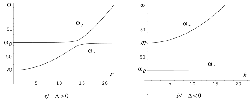
Figure 1: Dispersion curves for the photon like and dipole like excitations. Fig 1a shows the curves for red detuning ($\Delta=\omega_{0}-m>0$), where the photon branch corresponds to the curve $\omega_{-}$ for low momentum $k$ and to $\omega_{+}$ for high momentum. Fig 1b shows the curves for blue detuning ($\Delta=\omega_{0}-m<0$), where the photon branch corresponds to $\omega_{+}$ for all momenta. The curves are shown in dimensionless units with $|\Delta|=1$. The parameter values are $\omega_{0}=100$ and $\eta=0.1$.

For the case of interacting photons, just as for non-interacting photons, a low-momentum description can be made where the photons appear as non-relativistic, massive particles. Thus, when the photon frequency is separated from the resonance frequency of the oscillator mode by a detuning gap $\Delta=\omega_{0}-m_{0}$, and the transverse momentum is restricted by

$$\mbox{$$}k^{2}\ll m_{0}\Delta\ll\omega_{0}^{2}\ \,,$$ (18)

then the previous expressions for $S_{eff}^{(2)}$ and $S_{eff}^{(4)}$ ((8) and (9)) define a low momentum effective action for the photons, with a dispersion relation of a non-relativistic form

$$\mbox{$$}\omega(k)=m+\frac{k^{2}}{2m}+...\,.$$ (19)

In the following we shall in addition assume weak coupling between the photons and dipoles, in the sense

$$\mbox{$$}\eta^{2}\ll\Delta^{2}\ .$$ (20)

The effective photon mass is then given by

$$\mbox{$$}m^{2}=m_{0}^{2}-\eta^{2}\frac{m_{0}}{2\Delta}+...\,,$$ (21)

with a small renormalization of the mass due to the interaction with the dipole field. Note that the weak coupling condition (20) is not essential for the non-relativistic description of the 2D photons, but is introduced to simplify the calculations. In physical realizations of the 2D photon gas one may also have to consider the case of strong mixing of the photon and dipole degrees of freedom, as discussed in the section on Rydberg atoms below.

With the longitudinal momentum fixed to $m_{0}$ and $\omega(k)$ approximated by $m$, the field variable $A^{(-)}$ can be written as,

$$\mbox{$$}\vec{A}^{(-)}(\vec{r},z,t)=\sum_{a=\pm 1}\int\frac{d^{2}k}{(2\pi)^{2}}\frac{1}{\sqrt{mL}}\sin(m_{0}z)\left[e^{-i(mt-\vec{k}\cdot\vec{r})}\;\vec{\epsilon}_{a}(\vec{k})\,\phi_{a}(\vec{k},t)+c.c.\right]\,,$$ (22)

where $\vec{\epsilon}_{a}(\vec{k})$ are the polarization vectors and $\phi_{a}(\vec{k},t)$ are the corresponding field components, which now only depend on the transverse momentum $\vec{k}$. Note that both the frequency and the momentum of the longitudinal mode have been extracted from $\phi_{a}(\vec{k},t)$ in order to express this as a slowly varying field.

When the assumptions about small transverse momentum and weak coupling are imposed, the quadratic part of the effective action gets the form (to order $k^{2}$),

$$\mbox{$$}{\cal S}_{\phi}^{(2)}=\int d^{2}rdt\,\sum_{a=\pm 1}\left[\frac{i}{2}\left(\phi_{a}^{*}\dot{\phi}_{a}-\dot{\phi}_{a}^{*}\phi_{a}\right)-\frac{1}{2m}\left|\vec{\nabla}\phi_{a}\right|^{2}\right]$$ (23)

Here we have neglected terms proportional to $\dot{\phi}/m$ (slowly-varying field approximation), and $\vec{\nabla}$ is now the two-dimensional gradient. Note that the two polarization directions appear as two species of particles. The action has the standard form of a non-relativistic, free field theory.

We will now consider the interaction term. In the same approximation as used above we have

$$\mbox{$$}\frac{1}{\sqrt{(\omega_{-}(k)^{2}-\omega_{0}^{2})^{2}+\eta^{2}\omega_{0}^{2}}}\approx\frac{1}{2m|\Delta|}\,.$$ (24)

If this $k$-independent expression is used in the interaction part of the action, (9), and the $\vec{E}^{(-)}$ field is expressed in terms of $\phi_{a}$, it simplifies to

$$\mbox{$$}{\cal S}_{\phi}^{(4)}=-\frac{\pi g}{2m}\int d^{2}rdt\,\sum_{a=\pm 1}\left[|\phi_{a}|^{4}+2|\phi_{a}|^{2}|\phi_{-a}|^{2}\right]\,.$$ (25)

where $g$ is the (bare) interaction strength given by

$$\mbox{$$}g=\frac{1}{(2\pi)^{2}}\frac{3}{16}\frac{\Lambda}{\rho}\left(\frac{\eta}{\Delta}\right)^{4}\,.$$ (26)

The first term of (25) can be interpreted as a delta function interaction between photons with the same helicity, the second between photons of opposite helicities. In the simplest case, with only one type of photon polarization ($\phi_{a}=\phi$), the corresponding interaction Lagrangian simplifies to

$$\mbox{$$}{\cal L}_{\phi}^{(4)}=-\frac{\pi g}{2m}|\phi(\vec{r},t)|^{4}\,.$$ (27)

Thus, with the approximations used, we reach a form of the effective photon Lagrangian which agrees with the nonlinear Schrödinger equation previously derived from the classical field theory of a dimensionally reduced Maxwell field interacting with a non-linear medium Akhmanov . The photons behave like 2D massive particles with a repulsive, pointlike interaction.

In the case of blue detuning, i.e., $\Delta<0$, the situation is quite different. Typical dispersion curves are shown in Fig.1b, and we see that now the $\omega_{+}(k)$ branch is photon-like both for small and large momenta, and there is no avoided level crossing, but only a level repulsion at small momenta.

However, also for blue detuning a low momentum effective action can be given where all the above formula, derived for red detuning, still hold for scattering between the photons. But an important change is that the photons now are the “high energy” particles relative to the dipoles, and it is energetically possible for them to “decay” into the low lying dipole modes. At tree level (to first order in the interaction) the dangerous process is $\gamma\gamma\rightarrow\gamma{\rm D}$ which for blue detuning can conserve both energy and momentum. The corresponding interaction piece in the Lagrangian can again be read from (16), but now with one of the fields as $\vec{E}^{(-)}$ (dipole field) and the three others as $\vec{E}^{(+)}$ (photon field). In the low momentum approximation it is

$$\mbox{$$}{\cal L}_{\rm mix}^{(4)}=-\frac{\pi g}{m}\frac{\Delta}{\eta}(\tilde{\phi}^{*}\phi)(\phi^{*}\phi)\,,$$ (28)

where $\phi$ is the photon field and $\tilde{\phi}$ is the dipole field.

An important quantity for assessing whether a gas of blue detuned photons can be maintained in the cavity, is the ratio between the cross section of the above (‘inelastic’) decay process, and the normal (‘elastic’) scattering $\gamma\gamma\rightarrow\gamma\gamma$ induced by the interaction (26). A straightforward calculation yields,

$$\mbox{$$}\sigma_{tot}^{el.}(k) = \frac{1}{2}\left(\pi g\right)^{2}\frac{1}{k}$$ (29)

$$\sigma_{tot}^{inel.}(k) = \left(\frac{\pi g\Delta}{\eta}\right)^{2}\sqrt{\frac{2}{m|\Delta|}}$$

where $k$ is the momentum in the center of mass. Thus, demanding $\sigma_{tot}^{inel.}\ll\sigma_{tot}^{el.}$, implies the condition

$$\mbox{$$}k\ll\left(\frac{\eta}{\Delta}\right)^{2}\sqrt{\frac{m|\Delta|}{8}}\,.$$ (30)

We shall return to numerical estimates of the physical parameters in section 7.

We conclude this section with some comments on Galilean invariance. The effective action, given by (8) and (9), is neither Lorentz nor Galilean invariant, since the relativistic photons are coupled to dipoles defined in a fixed frame. Nevertheless the effective theory defined by (23) and (25) is Galilean invariant due to the low momentum approximations made in the vertices. In the next section we will consider loop effects where the low momentum approximations are not any longer valid, and it is far from obvious that the resulting corrections to the effective theory will respect the Galilean invariance. As we shall see, however, the leading corrections do have this symmetry, so the interpretation of the photons as a nonrelativistic Bose system has validity beyond the Born approximation.

IV 4 Renormalization of the $\delta$-function interaction.

In a many-particle interpretation the interaction Lagrangian (27) corresponds to a delta-function potential

$$\mbox{$$}V(r)=\frac{\pi g}{m}\sum_{i<j}\delta^{(2)}(\vec{r}_{ij})$$ (31)

where $\vec{r}_{ij}$ is the two-particle relative position. However, it is well known that a pure delta function interaction in dimensions higher than one is not well defined beyond first order in perturbation theory. In two dimensions the second order term gives rise to a logarithmic divergence in the scattering amplitude. To make the delta function interaction meaningful requires regularization of the interaction and renormalization of the interaction strength. As discussed in ref.jackiw1 the form of the s-wave scattering amplitude for such a renormalized interaction is

$$\mbox{$$}f(k)=-(2\pi)^{2}\sqrt{\frac{1}{2\pi k}}\,\frac{\frac{g_{r}}{4}}{1-\frac{g_{r}}{4}\left(\ln\frac{k^{2}}{\mu_{r}^{2}}-i\pi\right)}$$ (32)

where $g_{r}$ is the renormalized coupling constant and $\mu_{r}$ is a new parameter that is introduced by the renormalization (the renormalization scale). The corresponding phase shift for small $g_{r}$ is given by $\delta_{0}=\pi g_{r}/4$, which is the Born approximation value when $g=g_{r}$. For small valus of $k$ it approaches the universal expression, $\delta_{0}\approx\pi/\ln k^{2}$, that is common for a large class of short range potentials chadan98 .

Formally, the delta function interaction in two dimensions is dimensionless, i.e., it scales as the kinetic energy. However, the renormalization breaks the scaling symmetry and introduces a length scale through the parameter $\mu_{r}$. This is similar to the situation in QCD, where the effect is referred to as dimensional transmutation thorn . One should note that the two parameters $g_{r}$ and $\mu_{r}$ are not independent. Thus, $g_{r}$ may be fixed as the bare parameter $g$ and all the effect of the renormalization may be absorbed in $\mu_{r}$, or $g_{r}$ may be viewed as depending on $\mu_{r}$, where $\mu_{r}$ is chosen to match the physical momentum interval. In the latter case $g_{r}$ is referred to as an effective (or running) coupling constant. The explicit dependence on $\mu_{r}$ is given by

$$\mbox{$$}{\frac{1}{g}_{r}}={\frac{1}{g}}-\ln{\frac{\mu_{r}^{2}}{\mu_{0}^{2}}}$$ (33)

with $\mu_{0}$ as a constant. From this expression we notice that for large momenta (large $\mu_{r}$) the effective coupling constant goes to zero, so this is a quantum mechanical analogue of the asymptotic freedom of QCD. Note also the curious fact that for sufficiently large $k$ the effective interaction is always attractive, irrespectively of the sign of the bare parameter $g$, whereas it in the other limit is repulsive.

The above discussion refers to a situation where the $\phi^{4}$ theory is treated as a fundamental theory where $g_{r}$ and $\mu_{r}$ are free parameters, to be determined by experiment. However, treated as a an effective (low energy) theory they are in principle determined by the physical parameters of the complete system. For example, in the case of a quasi two-dimensional atomic Bose gas in a highly asymmetric trap, the renormalization scale of the two-dimensional theory is essentially given by the extension of the trap perpendicular to the plane in which the atoms move petrov ; hansson1 .

In the present case the renormalized interaction strength may be determined by taking more explicitly into account the effect of the dipole degrees of freedom. This we do by using Schrödinger perturbation thery, with the interaction Hamiltonian extracted from the the action (16), to calculate contributions to the scattering amplitude beyond the Born approximation. With the expression for the scattering amplitude given by (32), which we assume to be correct for low momenta $k$, we note that the renormalization scale $\mu_{r}$ can be determined from the contribution to second order in $g$ (with $g_{r}=g$). In such a second order calculation of the scattering amplitude the contributions from the dipole mode cannot be neglected, since the intermediate states are not restricted to low momenta. Thus, both the field modes $\vec{E}^{(\pm)}$ are included in the calculation, and the exact expressions for the mode frequences $\omega_{\pm}(k)$ are used rather than the low momentum approximations.

In the following we present a simple calculation of the leading contributions to the scattering amplitude. The result shows that the form of the amplitude is as expected and it gives an estimate of the renormalization scale $\mu_{r}$. In Appendix B we perform a more complete calculation of some of the non-leading terms in the scattering amplitudes and give the corresponding expressions for the scattering amplitude, for both red and blue detuning.

V 5 The scattering amplitude to $O(g^{2})$.

Consider the T-matrix, related to the scattering matrix by $S_{fi}=\delta_{fi}-2\pi i\delta(E_{f}-E_{i})T_{fi}$, where $E_{f}$ and $E_{i}$ are the energies of the final and initial states. To second order $T_{fi}$ has the form

$$\mbox{$$}T_{fi}=\langle k^{\prime}_{1}k^{\prime}_{2}|H_{int}|k_{1}k_{2}\rangle+\frac{1}{2}\int d^{2}p_{1}d^{2}p_{2}\frac{\langle k^{\prime}_{1}k^{\prime}_{2}|H_{int}|p_{1}p_{2}\rangle\langle p_{1}p_{2}|H_{int}|k_{1}k_{2}\rangle}{\omega(k_{1})+\omega(k_{2})-\omega(p_{1})-\omega(p_{2})+i\ e}$$ (34)

where we here have simplified the notation by the sum over field modes, longitudinal momenta and polarization variables in the intermediate state. The form of the interaction matrix element is

$$\mbox{$$}\langle p_{1}p_{2}| H_{int} |k_{1}k_{2}\rangle=\frac{1}{(2\pi)^{3}}\frac{\Lambda\eta^{4}}{2\rho\Delta^{2}}\delta(k_{1}+k_{2}-p_{1}-p_{2})(\delta_{n_{1}n_{2}}+\frac{1}{2}\delta_{n_{1}1}\delta_{n_{2}1}-\delta_{n_{1}n_{2}-2})$$ (35)

$$\times \sqrt{\frac{\omega(p_{1})}{(\omega(p_{1})^{2}-\omega_{0}^{2})^{2}+\eta^{2}\omega_{0}^{2}}\;\frac{\omega(p_{2})}{(\omega(p_{2})^{2}-\omega_{0}^{2})^{2}+\eta^{2}\omega_{0}^{2}}}\;\vec{e}^{\;*}\cdot\vec{e}_{\alpha}(\vec{p}_{1})\;\;\vec{e}^{\;*}\cdot\vec{e}_{\beta}(\vec{p}_{2})$$

where we have approximated the energy of the incoming photons $(k_{1}$ and $k_{2}$) by $m$, since these are in the lowest longitudinal mode. These photons have the same polarization vector $\vec{e}$, while the particles (“polaritons”) in the intermediate state have polarization vectors $\vec{e}_{\alpha}(\vec{p}_{1})$ and $\vec{e}_{\beta}(\vec{p}_{2})$. The quantum numbers $n_{1}$ and $n_{2}$ determine the longitudinal momenta of the particles in the intermediate state.

In the low-momentum approximation the T-matrix element is independent of the sum of the transverse momenta, $\vec{K}=\vec{k}_{1}+\vec{k}_{2}$, i.e., it is Galilean invariant. This follows since $\omega(k_{1})$ and $\omega(k_{2})$ can be approximated by $m$ in all places, except in the energy denominator when the intermediate particles are also in the lowest longitudinal mode. In that case the pole at $p_{1}^{2}+p_{2}^{2}=k_{1}^{2}+k_{2}^{2}$ makes the $k$-dependence important. However, due to momentum conservation, we have in the low-energy approximation

$$\mbox{$$}\omega(k_{1})+\omega(k_{2})-\omega(p_{1})-\omega(p_{2}) = \frac{1}{2m}(k_{1}^{2}+k_{2}^{2}-p_{1}^{2}-p_{2}^{2})$$ (36)

$$= \frac{1}{2m}(2k^{2}-2(\vec{p}_{1}-\frac{1}{2}\vec{K})^{2})$$

where $\vec{k}=\frac{1}{2}(\vec{k}_{1}-\vec{k}_{2})$ is the relative momentum. The expression shows that $\vec{K}$ can be absorbed in the integration variable $\vec{p}_{1}$.

Thus, the T-matrix has the following momentum dependence

$$\mbox{$$}T_{fi}=\delta(\vec{K}_{f}-\vec{K}_{i})\,{\cal T}(\vec{k}_{f},\vec{k}_{i})$$ (37)

where $\vec{K}_{f}$ and $\vec{K}_{i}$ are the sum of momenta for the outgoing and incoming particles and $\vec{k}_{f}$ and $\vec{k}_{i}$ are the relative momenta. For pure s-wave scattering (delta function interaction) the reduced T-matrix element ${\cal T}$ only depends on the magnitude of the relative momentum,

$$\mbox{$$}{\cal T}(\vec{k}_{f},\vec{k}_{i})={\cal T}(k^{2})$$ (38)

and is related to the s-wave scattering amplitude through

$$\mbox{$$}f(k^{2})=-(2\pi)^{2}m\sqrt{\frac{1}{2\pi k}}{\cal T}(k^{2})$$ (39)

Since we are interested in the behaviour of the scattering amplitude for small transverse momenta, in the first order expression we simply put them equal to zero. With all photons in the same helicity state, the first order contribution is

$$\mbox{$$}{\cal T}_{1}(k^{2})=\frac{g}{2\pi m}$$ (40)

in accordance with the expression for the low-energy Lagrangian (27). To second order there are three diagrams shown in fig. 2. Diagram 2a corresponds to two particles in the intermediate states, while diagrams 2b and 2c correspond to four and six particles in the intermediate states. Thus, the contributions from diagrams 2b and 2c are suppressed by the energy denominator, since the energy difference between the two initial and the four or six intermediate particles necessarily has to be large on the scale set by the transverse momentum. For this reason we shall only consider contributions from diagram 2a. Note that there are two types of particles in the intermediate state, characterized by energies $\omega_{-}$ and $\omega_{+}$. As an important point also note that the transverse momenta of the intermediate particle states cannot be assumed to be small, and also excitations to higher longitudinal momenta have to be considered. We now discuss how to calculate the leading contributions to diagram 2a.

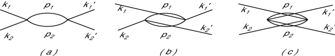
Figure 2: Second order contributions to the scattering amplitude. Only contributions from diagram (a) are included in this paper, since the contributions from (b) and (c) are suppressed by a factor $\Delta/m$.

At low momenta, there is a potentially large contribution to diagram 2a, when the energy denominator vanishes, and as expected this will give rise to the logarithmically infrared divergent term $\sim\ln k^{2}$ in (32). This term is dominant in the limit of asymptotically small momenta where the approximations leading to (16) become exact.

The importance of the high momentum contribution comes from the fact that $\omega_{-}$ does not increase with momentum, but rather approaches the resonance value $\omega_{0}$, c.f. Fig. 1. Thus, even if intermediate states with frequencies close to $\omega_{0}$ are considered as highly excited relative to the low energy photons, the large number of dipoles may make contributions from these modes important. In fact, if the dipoles are treated as a continuum, the integral over intermediate momenta will diverge. In reality we know that there is a physical cutoff related to the discreteness of the system of dipoles. We introduce this simply as a cutoff in momentum at a value corresponding to the (average) distance between the dipoles.

With a clear separation of the scales in the momentum integrals the leading contributions from high and low momenta can be estimated separately. In order to see how this works we examine the following toy problem. Consider the integral

$$\mbox{$$}I=\int_{0}^{\Lambda^{2}}dx\,\frac{1}{x+p^{2}}\frac{m^{4}+x^{2}}{x+\Delta^{2}}$$ (41)

which can be evaluated exactly, to give

$$\mbox{$$}I=\Lambda^{2}+\frac{1}{{p^{2}}-{{\Delta}^{2}}}\Big{(}{m^{4}}\log\big{[}\frac{{p^{2}}({{\Delta}^{2}}+{{\Lambda}^{2}})}{{{\Delta}^{2}}({p^{2}}+{{\Lambda}^{2}})}\big{]}+{p^{4}}\log\big{[}\frac{{p^{2}}}{{p^{2}}+{{\Lambda}^{2}}}\big{]}-{\Delta^{4}}\log\big{[}\frac{{\Delta^{2}}}{{\Delta^{2}}+{{\Lambda}^{2}}}\big{]}\Big{)}$$ (42)

However, assuming

$$\mbox{$$}p^{2}\ll\Delta^{2}\ll m^{2}\ll\Lambda^{2}\,$$ (43)

the integral can be estimated by the following approximation,

$$\mbox{$$}I \approx \int_{0}^{\Delta^{2}}dx\,\frac{1}{x+p^{2}}\frac{m^{4}+x^{2}}{x+\Delta^{2}}+\int_{m^{2}}^{\Lambda^{2}}dx\,\frac{1}{x+p^{2}}\frac{m^{4}+x^{2}}{x+\Delta^{2}}$$

$$\approx \frac{m^{2}}{\Delta^{2}}\int_{0}^{\Delta^{2}}dx\,\frac{1}{x+p^{2}}+\int_{m^{2}}^{\Lambda^{2}}dx\,1$$

$$\approx -\frac{m^{4}}{\Delta^{2}}\ln\frac{p^{2}}{\Delta^{2}}+\Lambda^{2}\,,$$

where the low and high momentum contributions are treated separately. This expression reproduces the exact result up to $O(m^{2}/\Lambda^{2})$. Below we will examine the leading contributions to the second order scattering amplitude in this way, by evaluating separately the contributions from low and high momenta. In this calculation the detuning parameter and the photon mass will play the role of $\Delta$ and $m$ in the toy problem. We refer to Appendix B for a more complete treatment.

V.1 The high-momentum contribution

For large momenta the important contribution comes from the term with two dipole excitations in the intermediate state. For these excitations we have have $\omega(p)^{2}\approx\omega_{0}^{2}$ and the momentum integral is divergent without the cutoff. The only effect of the coupling between the photons and the oscillators appears in the denominators of the form

$$\mbox{$$}\frac{1}{(\omega(p)^{2}-\omega_{0}^{2})^{2}+\eta^{2}\omega_{0}^{2}}\rightarrow\frac{1}{\eta^{2}\omega_{0}^{2}}$$ (45)

where it prevents the expression from diverging when $\omega(p)\rightarrow\omega_{0}^{2}$.

We can neglect contributions from the transverse momenta of the scattered (external) photons, since these are smaller by ${\cal O}[(k/m)^{2}]$ relative to the leading term. This means that the contribution gives rise to a $k$-independent renormalization of the interaction strength. We also neglect terms that are higher order in the coupling strength $\eta$. With $\omega(k)=m$ for the external photon states and $\omega(p)=\omega_{0}$ for the intermediate states the energy denominator is approximated by

$$\mbox{$$}\frac{1}{\omega(k_{1})+\omega(k_{2})-\omega(p_{1})-\omega(p_{2})}\rightarrow-\frac{1}{4m\Delta}$$ (46)

and the matrix elements of the interaction get a simple form

$$\mbox{$$}\left\langle{p_{1},p_{2}}\right|H_{int}\left|{k_{1}\,k_{2}}\right\rangle = \frac{\Lambda\eta^{2}}{2(2\pi)^{3}\rho\Delta^{2}\omega_{0}}\;\;\vec{e}^{\;*}\cdot\vec{e}_{\alpha}(\vec{p}_{1})\;\;\vec{e}^{\;*}\cdot\vec{e}_{\beta}(\vec{p}_{2})$$ (47)

$$\times \delta(\vec{p}_{1}+\vec{p}_{2}-\vec{k}_{1}-\vec{k}_{2})(\delta_{n_{1}n_{2}}+\frac{1}{2}\delta_{n_{1}1}\delta_{n_{2}1}-\delta_{n_{1}(n_{2}-2)})$$

For high momenta the summation over the polarization vectors gives simply a factor $3/4$ for each intermediate particle (as discussed in Appendix B) and the momentum integral and sum therefore gets trivial, with a momentum-independent matrix element. Integrating over transverse momenta and summing over longitudinal momenta gives

$$\mbox{$$}{\cal T}_{2a}(k^{2})=-\frac{3\pi}{64}\frac{\Lambda}{m^{2}\Delta}{\cal T}_{1}\equiv\alpha{\cal T}_{1}\,,$$ (48)

where $\alpha$ is a new dimensionless parameter. Since the dimensional reduction is not effective at high momenta (we have to sum also over the longitudinal momenta) this parameter is a characteristic of the full three-dimensional theory, and is a measure of the importance of renormalization of the nonlinear effects for intermediate momenta, i.e., for $g\ln k^{2}\Delta^{2}\ll\alpha$.

In order to obtain the finite result (48) we have introduced a cutoff, $p_{max}=\pi/l_{osc}$, in the momentum integration, where $l_{osc}=\rho^{-\frac{1}{3}}$ is the distance between the oscillators, and a cutoff in the discrete longitudinal momentum variable at $N=L/l_{osc}=L\pi p_{max}$. This means that we have $(p_{max}/\pi)^{3}=\rho$, with $\rho$ as the 3D oscillator density.

V.2 The low-momentum contribution

The important low momentum contribution comes from the term with two photons in the intermediate state. The energy denominator then vanishes when the momenta of the intermediate photons match the ones of the external photons. Since all photons then are low momentum photons, for the leading contribution we can replace $\omega(p)$ by the low energy expression $m+p^{2}/2m$ (and $\omega(k)$ by $m+k^{2}/2m$) to get the energy denominator on the form

$$\mbox{$$}\frac{1}{\omega(k_{1})+\omega(k_{2})-\omega(p_{1})-\omega(p_{2})}\rightarrow\frac{2m}{k_{1}^{2}+k_{2}^{2}-p_{1}^{2}-p_{2}^{2}}\,.$$ (49)

Here $p_{1}$ and $p_{2}$ are the transverse photon momenta of the intermediate state. In this case only the lowest longitudinal mode has to be included in the intermediate state. In the same way as for high momenta there are corrections, but they are supressed by factors $\eta^{2}/m^{2}$ or $\Delta^{2}/m^{2}$, and we shall neglect them.

We note that an integration of the intermediate state momentum of this term alone gives rise to a logarithmic ultraviolet divergence. Eventually this divergence is of course cut off by the interparticle distance, but before that the integrand is suppressed by the factor

$$\mbox{$$}\sqrt{\frac{\omega(p)}{(\omega(p)^{2}-\omega_{0}^{2})^{2}+\eta^{2}\omega_{0}^{2}}}\approx\sqrt{\frac{m}{(2m\Delta-p^{2})^{2}+\eta^{2}\omega_{0}^{2}}}$$ (50)

which will introduce an effective cutoff in the momentum integral at $2m|\Delta|$ and thus provide a scale for the logarithm. If this is introduced as an explicit cutoff, the momentum integral, after the angular integration, gets the form

$$\mbox{$$}I = 2\pi\int_{0}^{2m|\Delta|}dp^{2}\frac{1}{(k^{2}-p^{2}+i\epsilon)}=-\frac{1}{(2m\Delta)^{4}}\left(\ln\frac{k^{2}}{2m|\Delta|}-i\pi\right)$$ (51)

There will also be a constant ($k$ independent) contribution, but as shown explicitly in Appendix B this is generally small compared to the leading high momentum contribution (48). With the relevant constants and symmetry factors included, the logarithmic contribution to ${\cal T}$ is, for red and blue detuning,

$$\mbox{$$}{\cal T}_{2c}(k^{2})=\frac{g}{4}\left(\ln\frac{k^{2}}{2m|\Delta|}-i\pi\right){\cal T}_{1}$$ (52)

There is also a term corresponding to one photon and one dipole in the intermediate state, but the real part of this is subleading relative to the terms already included and can therefore be omitted. However, for blue detuning it has an imaginary part

$$\mbox{$$}{\cal T}_{2b}^{blue}(k^{2})=i\pi g\left(\frac{\eta}{\Delta}\right)^{2}{\cal T}_{1}\,.$$ (53)

Although small compared to the leading contribution, this is the dominant imaginary part corresponding to the decay process $\gamma\gamma\rightarrow\gamma D$ discussed earlier. As a check on our calculations, we have verified that this imaginary part of the scattering amplitude is correctly related to the total inelastic cross section in (29).

V.3 The scattering amplitude

Combining (40), (48) and (52) we get the following approximation for the (one loop) scattering amplitude corresponding to red detuning

$$\mbox{$$}{\cal T}(k^{2})=\frac{g}{2\pi m}\left[1+\alpha+\frac{g}{4}\left(\ln\frac{k^{2}}{2m\Delta}-i\pi\right)\right]\,.$$ (54)

The expression is consistent with the expression for the scattering amplitude of a renormalized delta function interaction, when expanded to second order in the coupling strength. Resumming the diagram 2a as a geometrical series in fact gives the full scattering amplitude (32), if we set $g_{r}=g$ and define the renormalization scale $\mu_{r}=\mu_{0}$ by

$$\mbox{$$}\mu_{0}^{2}=2m|\Delta|e^{-\frac{4\alpha}{g}}\,.$$ (55)

The same expression is valid for blue detuning if we neglect the effect of scattering $\gamma\gamma\rightarrow\gamma D$. Note, however, that the sign of $\alpha$ is different in the two cases. The value of the exponent is

$$\mbox{$$}-\frac{4\alpha}{g}=\frac{1}{2}(2\pi)^{3}\frac{\rho\Delta^{3}}{m^{2}\eta^{4}}$$ (56)

and we note that this (in absolute value) will be much larger than $1$ with the assumptions about parameter values which we have made.

The choice of renormalization scale, $\mu_{0}$ in (55) is however misleading in that the logarithm becomes large. The definition $\mu_{r}=2m|\Delta|$ amounts to a more natural choice since the interpretation of the photons as massive non-relativistic particles only makes sense for $k^{2}/(2m)<|\Delta|$. The corresponding value for the renormalized coupling constant is

$$\mbox{$$}g_{r}=\frac{g}{1-\alpha},$$ (57)

and relative to the bare (first order) coupling constant $g$, the change in $g_{r}$ remains small as long as the logarithm is small and $\alpha\approx\Lambda/(m^{2}\Delta)<<1$. But depending on the parameter values, $\alpha$ may in reality become large and give rise to a significant renormalization effect. For large $\alpha$ we have

$$\mbox{$$}g_{r}\approx-\frac{g}{\alpha}=\frac{1}{\pi^{3}}\frac{m^{2}\eta^{4}}{\rho\Delta^{3}}$$ (58)

and we note that in this limit the effective interaction is independent both of momentum and of the anharmonicity parameter $\Lambda$ of the oscillator spectrum. The detuning parameter $\Delta$ (and not the anharmonicity parameter $\Lambda$) now determines the sign of the effective coupling, with repulsive interaction for red detuning and attractive interaction for blue detuning.

V.4 Comparison with the Kerr nonlinear susceptibility coefficient $\chi^{(3)}$ for two-level atoms

Since the renormalization parameter $\alpha$ is proportional to $1/\Delta$, it easily gets large for small detuning, $\Delta<<\omega_{0}$, as shown explicitly for the case of photons interacting with Rydberg atoms, in the section below. The renormalized coupling constant $g_{r}$ (which then is much smaller than the bare coupling constant $g$) should then be interpreted as the physical interaction parameter. One should, however, note that the expression we have found for $g_{r}$ is not based on a systematic expansion in $\Lambda$, but rather by resumming “dangerous” terms in the expansion. There will be other contributions to the renormalized coupling, but these are parametrically small, i.e., supressed by powers of small ratios like $\eta/m$ or $\Delta/m$. Without resumming other parts of the perturbation series, we cannot determine in which parameter range these terms can be neglected. For the following estimates we shall simply assume that we are in that range.

The interpretation of $g_{r}$ as the physical interaction parameter is reinforced by the fact that the expression we have found (58), depends on the detuning parameter $\Delta$, the effective plasma frequency $\eta$, and the atomic number density $\rho$ in exactly the same way as the non-linear Kerr susceptibility coefficient $\chi_{G}^{(3)}$ for a dilute gas of two-level atoms, as obtained by Grischkowsky Grischkowsky ,

$$\chi_{G}^{(3)}=\frac{\rho\mu_{e}^{4}}{2\Delta^{3}}$$ (59)

with $\mu_{e}$ as the dipole matrix element (for one component of the dipole vector) connecting the two states of the two-level atom. Rewritten in our notation,

$$\mbox{$$}\mu_{e}^{2}=\frac{q^{2}}{M\omega_{0}}=\frac{\pi^{3}}{2}\frac{g_{r}}{m^{2}\omega_{0}^{2}}$$ (60)

which gives

$$\mbox{$$}\chi_{G}^{(3)}=\frac{\eta^{4}}{2\rho\omega_{0}^{2}\Delta^{3}}=\frac{\pi^{3}}{2\omega_{0}^{2}}g_{r}\text{ .}$$ (61)

To compare the expressions, we write the 3D susceptibility, extracted from our effective action (16), in terms of the dimensionless bare coupling constant $g$,

$$\chi^{(3)}=\frac{1}{16}\frac{\eta^{4}\Lambda}{\rho m^{4}\Delta^{4}}=\frac{(2\pi)^{2}}{3}\frac{g}{m^{4}}\,.$$ (62)

If we assume that the 3D susceptibility renormalizes in the same way as the 2D dimensionless $g$ (the renormalization comes from high $k$ where the dimensional reduction from 3D to 2D is not relevant), then

$$\mbox{$$}\chi_{r}^{(3)}=\frac{(2\pi)^{2}}{3}\frac{g_{r}}{m^{4}}=\frac{8}{3\pi}\left(\frac{\omega_{0}}{m}\right)^{2}\chi_{G}^{(3)}\,.$$ (63)

and since $m\approx\omega_{0}$, our expression for $\chi^{(3)}$ is very close to Grischkowsky’s.

That the factor $8/3\pi\approx.85$ is very close to one is of no significance, since our coefficient depends on the details of the ultraviolet cutoff. What is relevant, however, is that the two quite different approaches give essentially the same result for the susceptibility, and also that our result is independent of the bare non-linear coupling.

VI 6 Scales, Bose-Einstein condensation and two photon bound states

Based on the discussion of the effective photon-photon interaction in the previous sections, we will now consider some of the physical aspects of the formation of a two-dimensional photon fluid. We first summarize the important parameters that characterize the photon system, and then discuss the conditions under which two particularly interesting phenomena could occur: the formation of a two dimensional Bose-Einstein condensate, and the formation of two-photon bound states. We should stress that both these effects are essentially quantum mechanical, and cannot be described by classical non-linear optics.

VI.1 Important scales

The strength of the mixing between the photons and the oscillators is given by the effective plasma frequency $\eta$ defined by

$$\mbox{$$}\eta^{2}=\frac{\hbar cq^{2}\rho}{M}\,,$$ (64)

and mixing becomes important when $\eta^{2}\sim\Delta^{2}$. From now on we shall restore factors of $c$ and $\hbar$ in the formulas.

The (unrenormalized) interaction strength is given by the dimensionless coupling constant $g$,

$$\mbox{$$}g=\frac{1}{(2\pi)^{2}}\frac{3}{16}\frac{\hbar\Lambda}{c^{3}\rho}\left(\frac{\eta}{\Delta}\right)^{4}\,.$$ (65)

The importance of the non-linear loop corrections to the interaction strength is, for momenta $k^{2}\sim 2\hbar m\Delta$, determined by the dimensionless parameter $\alpha$,

$$\mbox{$$}\alpha=-\frac{3\pi}{64}\frac{\hbar^{3}\Lambda}{c^{4}m^{2}\Delta}\,.$$ (66)

and for large $\alpha$ the effective coupling constant is given by

$$\mbox{$$}g_{r}\approx\frac{1}{\pi^{3}}\frac{cm^{2}\eta^{4}}{\hbar^{2}\rho\Delta^{3}}\,.$$ (67)

Finally, for very small momenta, with

$$\mbox{$$}g\ln\frac{k^{2}}{2m\Delta}\sim 1+\alpha\,,$$ (68)

the logarithmic term will become important and contribute to the renormalization of the interaction.

VI.2 Photonic Bose-Einstein condensates

As mentioned in the introduction, one of the most exciting aspects of forming a photon gas, would be the possibility to study phase transitions. First, recall that there is no Bose-Einstein condensation (BEC) in a free two dimensional gas. However, the situation is different when the gas is in a trapping potential, where the transition temperature is given by $k_{B}T_{c}\approx\sqrt{N}\hbar\Omega$ Bagnato91 , where $N$ is the total number of bosons and $\Omega$ is the frequency of the (harmonic) trapping potential. In an interacting gas the situation is more complicated. The Mermin-Wagner theorem Mermin66 rules out true long-range order, but there is still the possibility of a Kosterlitz-Thouless (KT) transition, with the formation of a “quasicondensate” at a critical temperature $k_{B}T_{c}\approx\rho_{2D}\hbar^{2}/{m}$, with $\rho_{2D}$ the 2D boson density and $m$ the boson mass. In the context of two-dimensional atomic BEC, the phase transition in a quasi two dimensional Bose gas with repulsive delta function interactions was recently analyzed by Petrov, Holzmann and Shlyapnikov petrov . They find that in a trapping potential a true condensate will form well below $T_{c}$, whereas for intermediate temperatures $T<T_{c}$ it will change to a quasicondensate with a spatially fluctuating phase.

For a two-dimensional (dilute) photon gas a similar analysis should be relevant. We will make some comments on this in the discussion of a photon gas interacting with Rydberg atoms in the next section. For this discussion the expressions for the effective interaction parameter, (67) and the two-dimensional cross-section (29) are important. There are also important questions concerning the thermalization time and the possibility of regulating the effective temperature of the photon gas. With the parameter values discussed below the critical temperature is typically very much higher than the excitation energies. This indicates that a thermalized photon fluid would tend to form a Bose condensate rather than a normal fluid, and that the phase transition temperature cannot easily be reached by varying the parameter values of the photon fluid.

VI.3 A two-dimensional two photon bound state

The scattering amplitude (32) always has a pole for complex $k$ on the second Riemann sheet, at $k^{2}=-2mE_{b}$. This corresponds to a bound state, a “diphoton state” diphoton , with binding energy $E_{b}$ given by

$$\mbox{$$}E_{b}=\frac{\mu_{0}^{2}}{2m}e^{\frac{4}{g}}=|\Delta|e^{\frac{4}{g_{r}}}\,.$$ (69)

Somewhat surprisingly it looks like one could have a bound state for either sign of $g_{r}$, and this is indeed the case for a fundamental delta function interaction jackiw1 . We note, however, that for repulsive interactions ($g_{r}>0$), the bound state would occur at large $k$, far outside the range of validity of our effective theory. For attractive interaction ($g_{r}<0$) however, the presence of such a two photon bound state is a bona fide quantum mechanical effect with no obvious counterpart as a solution of the non-linear Schrödinger equation.

When $|\alpha|<1$, attractive interaction corresponds to negative $\Lambda$, and diphoton states could in principle form for red detuning, where the photons are stable against decay to the lower energy dipole mode. However, when $\alpha>>1$, which seems most relevant for physical realizations (se discussion below), weakly bound photon pairs would occur only for blue detuning. In this case we do not expect the formation of stable bound pairs due to the presence of the decay channel to the dipole mode.

VII 7 The 2D photon fluid: Physical realizations

In this section we shall discuss two possible experimental scenarios for the formation of a 2D photon fluid. First, we consider microwave photons in a cavity filled with Rydberg atoms. This scenario is quite close to the one described in the previous sections, since the highly excited atoms are well described as harmonic oscillators with a small anharmonicity. As a second example we shall consider optical photons in a cavity filled with alkali atoms in their ground states.

The question we shall address is the following: Can the parameters of these systems be tuned in such a way that there results a sufficiently large effective photon-photon interaction—mediated by virtual transitions within the atoms—so that a two-dimensional photon fluid can form within a Fabry-Perot resonator? One might expect that such a fluid arises after many effective photon-photon collisions within the cavity. Based on the analysis of the previous sections we reach an answer to this question which is qualified affirmative. The conditions for a photon fluid in thermal equilibrium to form may be met, but only under conditions where the parameters can be tuned to optimal values. For the Rydberg atoms these conditions seem more difficult to satisfy than for the optical photons.

However, the conclusions concerning the formation of a photon fluid are based on simple order of magnitude estimates of the physical parameters. One should note that the expressions used in these estimates were found above assuming certain conditions (separation of physical scales) which are not necessarily met in the real system. Also the expression found for the interaction parameter $g_{r}$ is based on the resummation of certain large contributions, while other higher order contributions are left out. For this reason we can present only a preliminary evaluation of the conditions for a 2D photon fluid to form. A detailed evaluation of these conditions is outside the scope of the present paper.

VII.1 Rydberg atoms in a microwave Fabry-Perot cavity: Numerical estimates

We first consider the case where microwave photons interact via Rydberg atoms excited near resonance, with both photons and atoms injected into a microwave version of a Fabry-Perot cavity. Consider a ribbon-shaped beam of Rydberg atoms passing through the gap between a pair of parallel, conducting plates, separated by a spacing $L_{L}\approx\lambda_{0}/2$. The plates are partially transparent to microwaves, for example, by having a regular square array of small holes, and can thus act as the (highly reflective) mirrors of a microwave Fabry-Perot cavity. Microwave photons can be injected into the cavity from the outside, and their transverse distribution, after many photon-photon interactions mediated by the atoms, can be monitored in transmission. The resonance frequency of the cavity can be tuned to near a resonance frequency of the Rydberg atoms.

For simplicity, let the plates be square in shape, with a typical transverse dimension of $L_{T}>>\lambda_{0}$, where $\lambda_{0}$ is the microwave resonance wavelength of the Rydberg atom transition of interest. The longitudinal mode number of the cavity is restricted to that of the fundamental longitudinal mode of the cavity (by our choice of spacing $L_{L}\equiv L=\lambda_{0}/2$ between the plates), but there can exist many possible transverse modes of the cavity, which are closely spaced near the fundamental longitudinal mode.

For concreteness, we shall use as a guide the parameters of the experiment of the Paris group Gawlik , where Rubidium atoms were excited to $n=50$, where $n$ is the principal quantum number of the Rydberg atom. The Rydberg atoms can be put into the “circular” state $|n,l=n-1,m=n-1\rangle$, which have a maximal electric dipole moment, and thus a maximal coupling to the microwave photons. Since the typical size of such a Rydberg atom is given by the radii of the circular Bohr orbits $a_{n}=n^{2}a_{0}$, where $a_{0}\approx 0.5$ Å is the Bohr radius, the atom can be quite large in size, e.g., $a_{n=50}\approx 0.125$ microns. The electric dipole transition matrix element for the $n=50\rightarrow n=51$ transition is also quite large, and therefore the photon-photon coupling mediated by such atoms virtually excited near resonance should be correspondingly large.

In the regime of high $n$, the energy levels of Rydberg atoms are almost equally spaced,

$$E_{n+\Delta n}=-\frac{\text{Ry}}{(n+\Delta n)^{2}}=E_{n}+\frac{2\text{Ry}}{n^{3}}\Delta n-\frac{3\text{Ry}}{n^{4}}\Delta n^{2}+\dots$$ (70)

where $Ry=13.6$eV is the Rydberg constant. The dominant photon-induced transitions will be between the circular states, $|n,n-1,n-1\rangle\rightarrow|n\pm 1,n\pm 1-1,n\pm 1-1\rangle$, where the wave function of the state $|n,n-1,n-1\rangle$ is

$$\mbox{$$}\psi_{n}(r,\theta,\psi)=\left[\frac{(2\kappa)^{3}}{8\pi n}\right]^{\frac{1}{2}}\frac{(-1)^{n-1}}{2^{n-1}(n-1)!}e^{-\kappa r}\,(2\kappa r)^{n-1}\,(\sin\theta)^{n-1}\,e^{i(n-1)\phi}\,,$$

with $\kappa=1/na_{0}$. This system is very well suited to be modeled by an anharmonic oscillator model of the type discussed earlier. We shall determine the anharmonic parameter $\Lambda$, the oscillator frequency $\omega$, and the oscillator mass $M$ of this model in terms of the Rydberg atom parameters, by matching the both the energy spectra to terms quadratic in $n$ and the dipole matrix elements between the levels $n$ and $n+1$.

One might object to this procedure since in our previous calculations we assumed the oscillators to be in their ground state rather than in a highly excited state. In particular this means that the effect of virtual transitions to lower Rydberg states that would be present in Rydberg atoms with the spectrum(70) are not taken into account. However, it should be kept in mind that the detuning for transitions of Rydberg atoms to lower states will be substantially larger than those to the higher states. In any case, for the simple numerical estimates made in this section we shall ignore this effect, and assume that only upward transitions $n\rightarrow n+1$ are important. This approximation will at most give rise to a numerical factor of order of unity in the estimate of the model parameters. For the same reason we shall neglect the fact that the oscillators of our model are three-dimensional and simply match the dipole matrix elements of the Rydberg states with those of the corresponding one-dimensional anharmonic oscillator.

With the above matching procedure for “circular” Rydberg atoms prepared in a state with the initial principal quantum number $n$, we get the following result for the anharmonicity parameter $\Lambda$ of the oscillator model

$$\Lambda=-\frac{8\omega_{0}^{2}\text{Ry}}{\hbar^{2}n^{4}}=-\frac{4\omega_{0}^{3}}{n\hbar}\text{ .}$$ (71)

However, this expression gives for the magnitude of the renormalization constant, $\left|\alpha\right|\simeq$ $\omega_{0}/(n\Delta)$, and $\alpha$ therefore becomes very large, since we shall operate the system with very small detunings near resonance, so that $\Delta<<\omega_{0}$. The detuning $\Delta$, however, must be much larger than the natural line width of the atoms Einstein-A , and in this limit we can use the $\Lambda$ independent expression (67) for the renormalized coupling constant. Note that in this limit the sign of the physical interaction is determined solely by the detuning parameter $\Delta$ - repulsive for red detunings $\Delta>0$, attractive for blue detunings, $\Delta<0$. Matching the dipole matrix elements effectively amounts to introducing a large oscillator strength, $f_{osc}=n^{2}(2n-1)/(n-1)^{2}$ in the expression for the effective plasma frequency $\eta=(q^{2}\rho/M)^{1/2}\rightarrow(\hbar ce^{2}f_{osc}\rho/m_{e})^{1/2}=c(\alpha_{e}f_{osc}\lambdabar_{C}\rho_{atom})^{1/2}$, where $\alpha_{e}$ is the fine structure constant, $m_{e}$ is the electron mass, and $\lambda_{C}=2\pi\lambdabar_{C}$ is the Compton wavelength of the electron. Although, strictly speaking, the detuning $\Delta$ should be much greater than the effective plasma frequency $\eta$, for the purposes of numerical estimates, we shall set $\Delta$ equal to $\eta$. Also, we shall approximate $mc^{2}\approx\hbar\omega_{0}$, where $\omega_{0}$ is the atomic resonance frequency of the transition in question. With this we get,

$$g_{r}=\left(\frac{2}{\pi}\right)^{3/2}\left(\frac{\alpha_{e}f_{osc}}{\rho_{atom}\lambda_{0}^{3}}\frac{\lambda_{C}}{\lambda_{0}}\right)^{1/2}\text{ ,}$$ (72)

where $\lambda_{0}$ is the atomic resonance wavelength of the transition in question.

As a first estimate of the size of $g_{r}$, consider the case of the the $n=50\rightarrow n+1=51$ “circular” Rydberg transition, where $mc^{2}/\hbar\approx\omega_{0}=2\pi\times 51$ GHz, with $\rho\simeq 1000$ atoms per $cm^{3}$ and $f_{osc}=105$. This yields an effective plasma frequency of $\eta\simeq 5.15\times 10^{6}s^{-1}$. For this transition, assuming that $\Delta\simeq\eta$, we find that $g_{r}\simeq 6.32\times 10^{-7}$.

VII.2 Cavity dimensions

To fit the frequency of the Rydberg transition $n=50\longrightarrow 51$, i.e., $\omega_{0}=51$ GHz, we assume the dimensions of the cavity to be chosen as follows,

$$L_{L}=\frac{1}{2}\lambda_{0}\approx 3\text{ mm and}\;L_{T}\approx 100\text{ cm,}$$ (73)

with $L_{L}=L$ as the longitudinal extension of the cavity and $L_{T}$ as the extension in the transverse directions. The limits for the transverse momentum $k_{T}=k$ are therefore

$$\frac{\pi}{L_{T}}<k_{T}<\left(2m\Delta\right)^{1/2}.$$ (74)

For a detuning $\Delta\simeq 2\pi\times 2$ MHz, this implies that there are around 10 nonrelativistic transverse modes in the cavity which can interact via the Rydberg atoms. Higher modes will be available and they will also interact via the atoms, but the energy-momentum relation for these higher modes will be modified relative to the non-relativistic expression. However, even with the limited number of modes available one should in principle be able to see the formation of a photon fluid in a Bose condensed state.

VII.3 The effective photon-photon collition rate and thermalization

We showed earlier that the total elastic cross-section in 2D is given by

$$\sigma^{el}\approx\frac{g_{r}^{2}}{k_{T}}\text{{.}}$$ (75)

The “reaction rate” for photon-photon collisions in 2D is therefore

$$\sigma^{el}v_{T}=\sigma^{el}\frac{\hbar k_{T}}{m}=\frac{\hbar}{m}g_{r}^{2}\text{ .}$$ (76)

The collision frequency $\omega_{coll}$ for photon-photon collisions in 2D is

$$\omega_{coll}=\rho_{2D}\sigma^{el}v_{T}=\rho_{3D}L_{L}\sigma^{el}v_{T}\text{ ,}$$ (77)

where $\rho_{2D}$ is the 2D photon number density, and $\rho_{3D}\,$is the 3D photon number density. Now the number of photon-photon collisions $N$ that occur within a cavity ring-down time $\tau$ is given by $N=\omega_{coll}\tau$, where, given the quality factor $Q$ of the cavity, $\tau=Q/\omega_{0}$. Solving for the number density of photons $\rho_{3D}$ needed for $N_{coll}$ photon-photon collisions, one obtains

$$\mbox{$$}\rho_{2D} = \frac{N}{Q\,g_{r}^{2}}{\left(\frac{\omega_{0}}{c}\right)}^{2}=4\pi^{2}\,\frac{N}{Q\,g_{r}^{2}}\,\lambda_{0}^{-2}$$

$$\rho_{3D} = 8\pi^{2}\,\frac{N}{Q\,g_{r}^{2}}\,\lambda_{0}^{-3}\,.$$ (78)

We note that due to the smallness of the interaction parameter ($g_{r}\simeq 6.3\times 10^{-7}$), there is a large numerical factor in these expressions. If we assume $N\simeq 10$ and a rather high quality factor of $Q\simeq 10^{7}$,

$$\mbox{$$}\frac{N}{Q\,g_{r}^{2}}=2.5\times 10^{6}$$ (79)

and the corresponding value of the photon density therefore gives a KT transition temperature far above the low-momentum regime of the interacting photons,

$$\mbox{$$}k_{B}T_{c}\approx\frac{\rho_{2D}\hbar^{2}}{m}\approx 2\times 10^{6}\,\hbar\omega_{0}$$ (80)

corresponding to a temperature $T_{c}\simeq 4\times 10^{6}$ K. Thus, the low-energy photons are typically in a temperature interval where a Bose condensate will form, rather than a normal fluid.

The microwave intensity inside the cavity is

$$\mbox{$$}I_{in}=\rho_{3D}\,c\,\hbar\omega_{0}$$ (81)

and with the given parameter values we find $I_{3D}\approx 1.1$ mW cm^-2. To convert from the inside-cavity to the outside-cavity intensity, we use the relation $I_{out}=I_{in}/Q$. Note that the incident power $I_{out}$ needed in order to form the photon fluid scales inversely as the $square$ of the quality factor, i.e., $I_{out}\sim Q^{-2}$, since $I_{in}$ is inversely proportional to $Q$.

Based on the above, we estimate that about 1.1 microwatts of incident microwave power is needed in order to get around ten photon-photon collisions within a cavity ring-down time of 30 microseconds. Under such circumstances, we expect that a 2D photon fluid should form inside the cavity.

The value of $Q\simeq 10^{7}$ is feasible ($Q\simeq 10^{8}$ by means of superconducting cavities have already been achieved Haroche ). Note, however, that if $\Delta>\eta$ the situation rapidly deteriorates due to the dependence on the factor $\left(\eta/\Delta\right)^{6}$ of $g_{r}^{2}$.

VII.4 Chemical potential and speed of sound of the photon fluid

From the previous section it might seem that it is always possible to form a photon fluid just by increasing the intensity of the incident microwaves. This conclusion is however not justified, since a too high intensity will make the fluid so dense, and the mean kinetic energy is so large, that the non-relativistic approximations are no longer valid. To get a rough estimate of when this happens, we use an effective Ginzburg-Landau (GL) type theory that should be applicable when the fluid is very dense. The relevant potential is given by

$$\mbox{$$}V=-\mu\left|\phi\right|^{2}+\pi g_{r}\frac{\hbar^{2}}{2m}\left|\phi\right|^{4}\approx 0\text{ .}$$ (82)

where we introduced a chemical potential which, in the Thomas-Fermi approximation, is related to the photon density by the relation

$$\mbox{$$}\mu=\pi g_{r}\frac{\hbar^{2}}{2m}\rho_{2D}\,,$$ (83)

which is obtained by minimizing $V$ with respect to $|\phi|^{2}=\rho_{2D}$. The GL theory defined by $V$ implies sound waves in the photon fluid with a speed given by Chiao2000 ,

$$\mbox{$$}v_{s}=\left(\frac{\mu}{m}\right)^{1/2}\text{ .}$$ (84)

We can also estimate the mean velocity of the photons using the virial theorem,

$$\mbox{$$}\langle E_{kin}\rangle=\frac{mv_{\gamma}^{2}}{2}\rho_{2D}=\langle E_{pot}\rangle=\mu\rho_{2D}$$ (85)

which gives $v_{gamma}=\sqrt{2}v_{s}$.

Imposing the consistency condition that $v_{s}=(\mu/m)^{1/2}<c$, we obtain an upper limit on the 2D photon number density that $\rho_{2D}<2m^{2}c^{2}/\hbar^{2}\pi g_{r}$. Combining this with the formation condition that $N>>1$, and using $\omega_{0}=mc^{2}/\hbar$, we obtain the upper and lower bounds on $\rho_{2D}$

$$\frac{m^{2}c^{2}}{\hbar^{2}Qg_{r}^{2}}<<\rho_{2D}<\frac{2m^{2}c^{2}}{\hbar^{2}\pi g_{r}}\text{ .}$$ (86)

We therefore conclude that a self-consistency condition for the formation of the photon fluid is

$$Q>>\frac{\pi}{2}g_{r}^{-1}\text{ .}$$ (87)

Thus, the choice of a high-$Q$ resonator is an important criterion for the formation of a photon fluid. For the case of the Rydberg transition $n=50\rightarrow 51$, we see that it would be necessary for $Q>>10^{6}$, so that the choice of $Q\simeq 10^{7}$ may be sufficient.

VII.5 Alkali atoms in an optical Fabry-Perot cavity

The apparent advantages of using microwaves and Rydberg atoms, rather than a more standard setup with lasers and e.g. Rubidium atoms, is twofold. First the cavity dimensions are not too small, and second, the large dipole moment of the atoms implies a large nonlinearity. The obvious disadvantage is that the Rydberg atoms are much harder to create and manipulate. Also since we have shown that the anharmonic parameter $\Lambda$ drops out of the renormalized coupling constant $g_{r}$ for small $\Delta$, it is of interest to consider an optical Fabry-Perot cavity with alkali atoms in their ground states, for which there is only a single transition to one excited state with a very strong oscillator strength of the order of unity, which almost completely exhausts the $f$-oscillator sum rule. For alkali atoms, a two-level model for the atom is therefore a more appropriate one Grischkowsky . However, the renormalized coupling constant for photon-photon interactions, and the resulting rates for collisions found in the previous section, should still apply here, provided that we remember to use the condition that the detuning $\Delta$ be comparable to the effective plasma frequency $\eta$ for the expressions for collision rates.

Consider the case of a fundamental longitudinal mode Fabry-Perot cavity with $L_{L}\approx\lambda_{0}/2$. In this case, the $Q$ of the cavity is also approximately its finesse. High quality mirrors with $Q\simeq 10^{5}$ are commercially available PMS . For a strongly allowed alkali transition, $f_{osc}\simeq 1$. If we assume a density $\rho_{atom}\simeq 10^{9}$ rubidium atoms per cm³ (rubidium atoms have a transition wavelength of $\lambda_{0}=780$ nm), this leads to an effective plasma frequency $\eta\simeq 2\pi\times 200$ MHz (which is comparable to the Doppler width of rubidium atoms at room temperature), With $\Delta\simeq\eta$ this gives $g_{r}\simeq 12\times 10^{-3}$. The minimum required $Q$ is therefore around 130, which is easily satisfied. Thus, if we set $N\simeq 10$ and $Q\simeq 10^{5}$, from Eq.(81) we obtain $I_{3D}\simeq 10^{6}$ W cm^-2, or an outside power requirement of a 0.1 Watt per square millimeter incident on the Fabry-Perot, which is feasible.

One consequence of going from microwave to visible wavelengths, is that the number of nonrelativistic transverse modes given by Eq.(74) can be much larger. For the given parameter values one finds that there are around 200 nonrelativistic transverse modes which can be coupled together. Also the estimated KT transition temperature is relatively lower, with $k_{B}T_{c}\approx 0.7\,\hbar\omega_{0}$.

VII.6 High-$Q$ microspheres of glass and the formation of a 2D photon fluid

Let us finally comment on a third possible way in which a 2D photon fluid could form. Extremely high-$Q$ optical cavities with $Q\simeq 10^{10}$ have been fabricated out of low-loss, small-diameter glass microspheres Ilchenko . A 120-$\mu$m diameter glass microsphere immersed in superfluid helium has been observed to exhibit a nonlinear, dispersive bistable behavior with a threshold power of as low as 10 microwatts, due to the intrinsic Kerr nonlinearity of the glass which constitutes the microsphere Haroche1998 . Due to the curvature of the microspheres the photons are tightly confined to propagate within an optical wavelength or so of the two-dimensional spherical surface, i.e., within its “whispering-gallery” modes. This tight, two-dimensional confinement of the light should also allow an effective dimensional reduction from 3D to 2D in the photon degrees of freedom, which differs from the mechanism of dimensional reduction in a planar Fabry-Perot cavity discussed here in this paper. Thus a two-dimensional photon fluid could also in principle form just within the inside surface of the microsphere, due to the photon-photon scatterings mediated by the intrinsic Kerr nonlinearity of the glass, and may have already been indirectly observed in the experiments of Haroche1998 . It should be noted that the change of topology from that of a plane to that of a sphere should not make the formation of the 2D photon fluid impossible in principle.

VIII 8 Concluding remarks

In this paper we used a microscopic approach to study the effective interaction between photons confined to a quasi-two-dimensional cavity filled with a non-linear medium. With the atoms modelled by a collection of non-linear Lorentz oscillators, the interaction was studied to second order in perturbation theory. The linear problem was first solved by decoupling the “polariton modes”, and we described efficient ways to do this, both by use of a path integral approach and by use of exact diagonalization, as shown in Appendix A. A main motivation was to examine the description of the effective interaction, induced by the non-linearity, as a 2D short range (delta function) interaction and to determine the renormalization scale associated with this interaction. We noticed several interesting complications. For red detuning relative to the oscillator frequency, the expression found to second order fits with the form of a normalized delta-function potential. However, the renormalization parameter is typically large and a resummation of “dangerous” terms has been performed in order to extract an effective, renormalized interaction strength. This way of including higher order contributions raises questions of whether other contributions, not included here (since they are parametrically small), may also be of importance. However, additional support for the expression found for the renormalized interaction parameter comes from other evaluations of the non-linear susceptibility of a gas of alkali atoms. For blue detuning, we discussed the possible formation of photonic bound states, and noticed the possibility that photons might “decay” into oscillator excitations.

The last part of the paper was devoted to a discussion of possible experimental scenarios, where a photon fluid may form in a Fabry-Perot resonator. In these cases, two-dimensionality is obtained by constraining the photons in one direction to their fundamental mode. By means of order of magnitude estimates we examined the constraints on the physical parameters in order for a photon fluid to form. There is a potential conflict between the need to have a high density of photons in order to obtain a satisfactory collision frequency and the possibility of having a too high density measured in units of the photon Compton wave length, since the effective photon mass is typically very small. For photons in a microwave cavity interacting with Rydberg atoms the corresponding constraints are serious, although by choosing optimal parameter values the conditions for creating a 2D photon fluid can probably be met. Such an experimental realization is otherwise attractive, as the model of photons interacting with Rydberg atoms is closely related to the oscillator model used in the paper. For photons in an optical cavity, the constraints on the physical parameters seem less severe, although the use of such small scale cavities may pose a larger experimental challenge. We noticed that in both cases the typical temperature associated with a Kosterlitz-Thouless phase transition lies well above the energy scale associated with non-relativistic 2D photons, and for such low energies a condensate will typically form if the collision frequency is sufficiently large on the scale set by the ringdown time of the cavity. In addition to the two possible experimental realizations discussed in some detail, we also suggest that other types of realizations of the 2D photon fluid may be possible, and in particular we pointed at the use of high-$Q$ microspheres of glass as being potentially interesting in this context.

Let us finally stress the point that in this study we have made some simplifying assumptions, in particular about a clear separation of the physical (energy) scales associated with the formation of a 2D photon fluid. In real systems, these conditions may not be well satisfied, and in the discussion of microwave photons interacting with Rydberg atoms we noticed that one may have to tune the frequency so close to the resonance value that the photons become strongly mixed with the oscillator degrees of freedom, i.e., they are genuine polaritons rather than photons. For this reason we consider the order of magnitude estimates applied to these realizations only as preliminary ones. A more detailed study is needed to settle more firmly the conditions for the creation of 2D photon fluids in such small Fabry-Perot cavities.

VIII.1 Acknowledgements

We thank John Garrison and Colin McCormick for helpful discussions. RYC acknowledges the partial support of this work by NSF grant PHY-0101501. JML thanks the Miller Institute for Basic Research in Science for financial support and hospitality. Supports from the Research Council of Norway and the US-Norway Fulbright Foundation are also acknowledged. THH thanks Nick Khuri and the theory group at Rockefeller University, as well as Shivaji Sondhi and the condensed matter group at Princeton University for hospitality.

IX Appendix A . Alternative derivation of the effective photon action

In this Appendix we derive the effective action (14) and (16) by an alternative method which does not require any field transformation of the type (13) which is non local in time. In addition to verifying the soundness of the simple procedure used in the text, the present derivation explicitly shows that the effective action is the sum of the two contributions in (14) and (16) corresponding to the two frequencies $\omega_{\pm}$.

The most natural object to consider given the action (1), would be the generating functional $Z[\vec{J}_{\vec{A}},\vec{J}_{\vec{R}}]$, which can be written as a Feynman path integral over the fields $\vec{A}$ and $\vec{R}$. By a change of variables one can diagonalize the quadratic part of the action, and then use perturbation theory to calculate Greens functions. However, becuause of the time derivative coupling (4), this will give rise to expressions which are nonlocal in time, since this procedure fails to correctly describe the normal modes. An obvious way to proceed is to switch to a Hamiltonian formalism, do an explicit diagonalization of the quadratic piece of the Hamiltonian by a symplectic transformation on the phase space, and finally express the nonlinear term in the new variables. This method is however cumbersome, and we now present a simpler approach based on the path integral.

The essential step is to use an alternative form of the action which is related to (1) by a Legendre transformation. Rather than just writing down this transformation, we shall go back to the derivation of the Feynman path integral, since this will illuminate the physical meaning of the new variables. The usual Hamiltonian description of (1) would comprise two canonical pairs $(\vec{A},-\vec{E})$ and $(\vec{R},\vec{P})$, where $\vec{P}=M\dot{\vec{R}}+q\vec{A}$. Since we are dealing with a coupled system of matter and radiation, it is rather natural to introduce the electric displacement vector by

$$\mbox{$$}\vec{D}=\vec{E}+q\rho\vec{R}=\nabla\times\vec{C}\,,$$ (88)

where the last identity defines the ”displacement vector potential” $\vec{C}$ provided that there are no macroscopic charges, i.e., $\nabla\cdot\vec{D}=0$. The variables $\vec{D}$ and $\vec{C}$ were used earlier by Hillery and Mlodinow in the context of quantization of non-linear electrodynamics hillery1984 . It is easy to show that $\vec{C}$ forms a canonical pair with the magnetic field strength $\vec{B}$. If we furthermore introduce the rescaled oscillator fields

$$\mbox{$$}\vec{Q} = \sqrt{\rho M}\vec{R}$$ (89)

$$\vec{\Pi} = \frac{1}{\sqrt{\rho M}}\vec{R}\,,$$

the canonical commutation relations take the form,

$$\mbox{$$}[B_{i}(\vec{r}),C_{j}(\vec{r}^{\prime})] = i\hbar\delta_{ij}\delta^{3}(\vec{r}-\vec{r}^{\prime})$$ (90)

$$\left[Q_{i}(\vec{r}),\Pi_{j}(\vec{r}^{\prime})\right] = i\hbar\delta_{ij}\delta^{3}(\vec{r}-\vec{r}^{\prime})\,,$$

and the corresponding quadratic Hamiltonian density is,

$$\mbox{$$}{\cal H}^{(2)}=\frac{1}{2}(\vec{B}^{2}+\vec{D}^{2})+\frac{1}{2}\left[\vec{\Pi}^{2}+(\omega_{0}^{2}+\eta^{2})\vec{Q}^{2}\right]-\eta\vec{D}\cdot\vec{Q}\,,$$ (91)

where again $\vec{D}=\nabla\times\vec{C}$, and $\eta^{2}=q^{2}\rho/M$. We now consider $\vec{B}$ and $\vec{\Pi}$ as the momenta and derive the path integral expression for the generating functional

$$\mbox{$$}Z[\vec{J}_{D}\vec{J}_{R}]=\int{\cal D}\vec{C}{\cal D}\vec{Q}\,e^{i{\cal S}[\vec{C},\vec{Q}]+i\int(\vec{J}_{D}\cdot\vec{D}+\vec{J}_{R}\cdot\vec{R})}\,,$$ (92)

by first writing a phase space path integral and then integrating over the momenta $\vec{B}$ and $\vec{\Pi}$. As we shall see below, the electric displacement field $\vec{C}$ will in the limit of weak coupling correspond to the photon, and the oscillator $\vec{Q}$ to the oscillating dipoles. At finite coupling these two modes mix and form two effective propagating ”polaritron” modes. In Fourier space, the quadratic part of the Lagrangian takes the form

$$\mbox{$$}{\cal L}^{(2)}=\frac{1}{2}\left(\matrix{C(-\vec{k})_{i}&Q(-\vec{k})_{i}}\right)\left(\matrix{P^{T}_{ij}(\omega^{2}-\vec{k}^{2})&i\epsilon_{ijk}\eta k_{k}\cr-i\epsilon_{ijk}\eta k_{k}&P^{T}_{ij}(\omega^{2}-\omega_{0}^{2}-\eta^{2})}\right)\left(\matrix{C(\vec{k})_{j}\cr Q(\vec{k})_{j}}\right)\,,$$ (93)

where $P^{T}_{ij}=\delta_{ij}-\hat{k}_{i}\hat{k}_{j}$ is a transverse projector. Since in this formulation, the dipole coupling term does not involve any time derivative, the quadratic part of the action can be diagonalized by a unitary transformaton which is local in time (although nonlocal in space):

$$\mbox{$$}\left(\matrix{C_{i}\cr Q_{i}}\right)=\left(\matrix{\cos\theta_{k}P^{T}_{ij}&-i\sin\theta_{k}\epsilon_{ijk}\hat{k}_{k}\cr i\sin\theta_{k}\epsilon_{ijk}\hat{k}_{k}&\cos\theta_{k}P^{T}_{ij}}\right)\left(\matrix{A^{(-)}_{j}\cr A^{(+)}_{j}}\right)$$ (94)

where

$$\mbox{$$}\cos\theta_{k}=\sqrt{\frac{\omega_{0}^{2}-\omega_{-}^{2}}{\omega_{+}^{2}-\omega_{-}^{2}}}$$ (95)

with $k^{2}=\vec{k}^{2}$ and, $\omega_{\pm}(k^{2})$ given by (12).

The resulting action is most conveniently expressed in spherical components defined by $R_{m}=\hat{e}_{m}^{*}\cdot\vec{R}$ etc. , with $\hat{e}_{m}^{*}\cdot\hat{e}_{m^{\prime}}=\hat{e}_{-m}\cdot\hat{e}_{m^{\prime}}=\delta_{mm^{\prime}}$, $\hat{k}\cdot\hat{e}_{m}=0$ and $m=\pm 1$. We get

$$\mbox{$$}{\cal L}^{(2)}(\vec{A}^{(+)},\,\vec{A}^{(-)})=\frac{1}{2}\sum_{m=\pm 1}A^{(+)}_{-m}(-\vec{k})(\omega^{2}-\omega_{+}^{2})A^{(+)}_{m}(\vec{k})+A^{(-)}_{-m}(-\vec{k})(\omega^{2}-\omega_{-}^{2})A^{(-)}_{m}(\vec{k})\,.$$ (96)

For the interaction term, we must express $\vec{R}$ in terms of $A^{(\pm)}$ using (94),

$$\mbox{$$}R_{m}(\vec{k})=\frac{1}{\sqrt{\rho M}}\left(\cos\theta_{k}A^{(+)}_{m}(\vec{k})+\sin\theta_{k}A^{(-)}_{m}(\vec{k})\right)\,,$$ (97)

where we also redefined $A^{(-)}_{\pm 1}(\vec{k})\rightarrow\pm A^{(-)}_{\pm 1}(\vec{k})$.

The final result for the generating function is,

$$\mbox{$$}Z[\vec{J}_{D},\vec{J}_{R}]=\int{\cal D}\vec{A}^{(+)}{\cal D}\vec{A}^{(-)}\,e^{i{\cal S}[A_{a}^{(+)},\,A_{a}^{(-)}]-i\int(\vec{J}_{D}\cdot\vec{D}+\vec{J}_{R}\cdot\vec{R})}\,.$$ (98)

with ${\cal S}[\vec{A}^{(+)},\vec{A}^{(-)}]={\cal S}^{(2)}+{\cal S}^{(4)}$ explicitly given by

$$\mbox{$$}{\cal S}_{eff}^{(2)} = \frac{1}{2}\int\frac{d^{3}k}{(2\pi)^{3}}\int\frac{d\omega}{2\pi}\,{\cal L}^{(2)}(\vec{A}^{(+)},\,\vec{A}^{(-)})$$ (99)

$${\cal S}_{eff}^{(4)} = -\frac{\rho\lambda M^{2}}{4!}\prod_{n=1}^{4}\left[\int\frac{d^{3}k_{n}\;d\omega_{n}}{(2\pi)^{4}}\right](2\pi)^{4}\delta(\sum_{n=1}^{4}\omega_{n})\delta(\sum_{n=1}^{4}\vec{k}_{n})$$

$$\times \vec{R}(\vec{k}_{1},\omega_{1})\cdot\vec{R}(\vec{k}_{2},\omega_{2})\,\vec{R}(\vec{k}_{3},\omega_{3})\cdot\vec{R}(\vec{k}_{4},\omega_{4})\,,$$

where $\vec{R}$ is given by (97). Note that the interaction is non local becauce of the $k^{2}$ dependence in the denominators in the $\cos\theta_{k}$ and $\sin\theta_{k}$ factors. Using the identities

$$\mbox{$$}\cos^{2}\theta_{k} = \frac{\eta^{2}\omega_{+}^{2}}{(\omega_{+}^{2}-\omega_{0}^{2})^{2}+\eta^{2}\omega_{0}^{2}}$$ (101)

$$\sin^{2}\theta_{k} = \frac{\eta^{2}\omega_{-}^{2}}{(\omega_{-}^{2}-\omega_{0}^{2})^{2}+\eta^{2}\omega_{0}^{2}}\,,$$

and substituting the expression (97) for $\vec{R}$ we recover (16).

X Appendix B. Scattering amplitude to second order

We perform here a more detailed evaluation of the second order contributions to the scattering amplitude. The contributions from low and high momenta of the intermediate states are examined, and we consider in both cases only the leading contributions in terms of the small quantities $k/m,\Delta/m$, and $\eta/\Delta$. The contributions come from diagram a) in Fig.2, with the intermediate lines corresponding to either the photon or the dipole mode, with transverse momenta running from zero to the cutoff $1/l_{osc}$, where $l_{osc}$ is the physical distance between the oscillators. There is also a sum over all longitudinal momenta, in terms of the discrete momentum variable $n$, and a sum over the polarization vectors of the fields.

The full expression for the interaction Hamiltonian is

$$\mbox{$$}H_{int}=K\prod\limits_{r=1}^{4}{\left[{\int{{{d^{2}k_{r}}\over{\left({2\pi}\right)^{2}}}}}\right]}\;\delta\left({\sum\limits_{r}{\vec{k}_{r}}}\right)\;\sum\limits_{\{n_{r}\}}{(\delta_{n_{1}+n_{2},n_{3}+n_{4}}+2\delta_{n_{1}+n_{3},n_{2}+n_{4}}-4\delta_{n_{1}+n_{2}+n_{3},n_{4}})}$$

$$\times\sum\limits_{\{i_{r}=\pm\}}\prod\limits_{r=1}^{4}[\Lambda_{i_{r}}\left({k_{r},n_{r}}\right)]{\vec{E}^{(i_{1})}(\vec{k}_{1},n_{1},t)\cdot\vec{E}^{(i_{2})}(\vec{k}_{2},n_{2},t)\vec{E}^{(i_{3})}(\vec{k}_{3},n_{3},t)\cdot\vec{E}^{(i_{4})}(\vec{k}_{4},n_{4},t)}$$ (102)

where $K=(2\pi)^{2}\Lambda\eta^{4}/(8\rho L)$ and $\Lambda_{\pm}\left({k,n}\right)=[\omega_{\pm}(k,n)^{2}-\omega_{0}^{2})^{2}+\eta^{2}\omega_{0}^{2}]^{-1/2}$ , $\;n_{r}(r=1,..,4$) is the summation variable for the longitudinal mode and $i_{r}$ for the photon/dipole mode. From this expression the T-matrix and the corresponding scattering amplitude can be determined. The T-matrix is related to the scattering matrix by $S_{fi}=\delta_{fi}-2\pi i\delta(E_{f}-E_{i})T_{fi}$, where $E_{f}$ and $E_{i}$ are the energies of the final and initial states, and to second order $T_{fi}$ has the form

$$\mbox{$$}T_{fi}=\langle k^{\prime}_{1}k^{\prime}_{2}|H_{int}|k_{1}k_{2}\rangle+\frac{1}{2}\int d^{2}p_{1}d^{2}p_{2}\frac{\langle k^{\prime}_{1}k^{\prime}_{2}|H_{int}|p_{1}p_{2}\rangle\langle p_{1}p_{2}|H_{int}|k_{1}k_{2}\rangle}{\omega(k_{1})+\omega(k_{2})-\omega(p_{1})-\omega(p_{2})+i\ e}$$ (103)

where we here have simplified the notation by suppressing the sum over field modes, longitudinal momenta and polarization variables in the intermediate state. Galilean invariance implies the following form

$$\mbox{$$}T_{fi}=\delta(K_{f}-K_{i}){\cal T}(k_{f},k_{i})$$ (104)

where $K_{f}$ and $K_{i}$ are the sum of momenta for the outgoing and incoming particles and $k_{f}$ and $k_{i}$ are the relative momenta. For pure s-wave scattering (delta function interaction) ${\cal T}$ only depends on the magnitude of the relative momentum,

$$\mbox{$$}{\cal T}(k_{f},k_{i})={\cal T}(k^{2})$$ (105)

and is related to the s-wave scattering amplitude through

$$\mbox{$$}f=-(2\pi)^{2}m\sqrt{\frac{1}{2\pi k}}{\cal T}(k^{2})$$ (106)

For the present case, the first order contribution to ${\cal T}$ is

$$\mbox{$$}{\cal T}_{1}=\frac{g}{2\pi m}=\frac{3}{16(2\pi)^{3}}\frac{\Lambda\eta^{4}}{m\rho\Delta^{4}}$$ (107)

With the interaction matrix elements evaluated and the sum over polarization performed, the expression for the second order contribution to ${\cal T}$ is

$$\mbox{$$}{\cal T}(k^{2}) = \frac{1}{2}C^{2}\sum_{n_{1}n_{2}}\sum_{i_{1}i_{2}}(\delta_{n_{1}n_{2}}+\frac{5}{4}\delta_{n_{1}1}\delta_{n_{2}1}+\delta_{n_{1}n_{2}-2})$$

$$\times \int d^{2}p\left[\frac{\omega_{i_{1}}(p,n_{1})}{((\omega_{i_{1}}(p,n_{1}))^{2}-\omega_{0}^{2})^{2}+\eta^{2}\omega_{0}^{2}}\;\frac{\omega_{i_{2}}(p,n_{2})}{((\omega_{i_{2}}(p,n_{2}))^{2}-\omega_{0}^{2})^{2}+\eta^{2}\omega_{0}^{2}}\right.$$

$$\times \left.\left(1-\frac{1}{2}\frac{p^{2}}{p^{2}+n_{1}^{2}m_{0}^{2}}\right)\left(1-\frac{1}{2}\frac{p^{2}}{p^{2}+n_{2}^{2}m_{0}^{2}}\right)\frac{1}{2\omega_{-}(k,1)-\omega_{i_{1}}(p,n_{1})-\omega_{i_{2}}(p,n_{2})+i\epsilon}\right]$$

. (108)

with $C=K/(4(2\pi)^{4}m\Delta^{2})$. Here the reference frame is chosen where the total transverse momentum vanishes. The energy of both incoming and scattered photons is $\omega_{-}(k,1)$, with the photons in the lowest longitudinal mode (and where red detuning has been assumed). Since these are low momentum photons, we have $\omega_{-}(k,1)\approx m+k^{2}/m$.

A simplification may be introduced by considering the effect of mixing between photons and dipoles, described through the parameter $\eta$. This mixing affects the expression in two ways. The first one is through the $\eta$ dependent term that is explicit in (X). This term is important when the particle energies are close to the resonance value $\omega_{0}$. The other one is the indirect one which enters through the particle energy $\omega_{\pm}$. When summing over both the photon and dipole modes in the intermediate state this $\eta$ dependence is less important. It only affects the lowest longitudinal mode and only for transverse momenta in a small interval $p\approx\Delta$. We will neglect this effect, which can be viewed as higher order in $\eta^{2}$ and use the energy expressions for the uncoupled modes,

$$\mbox{$$}\omega_{-} = \sqrt{p^{2}+n^{2}m_{0}^{2}}$$

$$\omega_{+} = \omega_{0}$$ (109)

(Note, with this redefinition $\omega_{-}$ is the photon mode also when higher in energy than the dipole mode.) We consider now separately contributions from the different modes in the intermediate states.

X.1 Two-dipole intermediate states

Since $\omega_{+}$ is independent of $p$ there is no suppression of the integrand for high momenta and the integral over $p$ and sum over $n$ are divergent without the momentum cutoff. This cutoff we set to $p_{max}$ for the transverse momentum and $N=p_{max}L/\pi$ for the longitudinal momentum. The connection with the oscillator density is $\rho=1/l_{osc}^{3}=(p_{max}/\pi)^{3}$. Since we assume $L>>l_{osc}$ most of the contribution comes from large transverse and longitudinal momenta where the dimensional reduction no longer is effective . We note that the only momentum dependence now sits in the polarization factor, which we approximate by

$$\mbox{$$}1-\frac{1}{2}\frac{p^{2}}{p^{2}+n^{2}m_{0}^{2}}=1-\frac{1}{2}\sin^{2}\theta\approx\frac{3}{4}$$ (110)

where $\theta$ is the angle between the momentum vector and the $z$-axis. In the last term we have approximated $\sin^{2}\theta$ by $1/2$ which is correct when we (for large momenta) can treat the longitudinal momentum as a continuous variable.

With these approximations the momentum sum and integral can trivially be performed, and the contribution is

$$\mbox{$$}{\cal T}_{2a} = -\frac{9}{32}C^{2}\pi Np_{max}^{2}\frac{1}{\Delta\eta^{4}\omega_{0}^{2}}$$ (111)

$$= -\frac{3\pi}{64}\frac{\Lambda}{m^{2}\Delta}{\cal T}_{1}$$

We note that the sign of this $k$-independent contribution depends on the sign of $\Delta$, the detuning parameter.

X.2 The photon-dipole contribution

We now consider the terms where one of the intermediate modes is a photon mode and the other a dipole mode. The momentum integral is convergent, with the main contribution coming from low momenta. For $p<<nm$ we approximate the polarization factors by 1, and ${\cal T}$ is simplified to

$$\mbox{$$}{\cal T}_{2b} = -2\pi C^{2}\frac{1}{\eta^{2}\omega_{0}^{2}}\sum_{n}(2+\frac{1}{4}\delta_{n1}-\delta_{n2})$$ (112)

$$\times \int_{nm}^{\infty}dp\left[\frac{p^{2}}{(p^{2}-\omega_{0}^{2})^{2}+\eta^{2}\omega_{0}^{2}}\;\frac{1}{p+\Delta-m-i\epsilon}\right]$$

The leading contribution (in $\Delta/m$) comes from the term $n=1$. Evaluation of the momentum integral gives for red detuning $\Delta>0$,

$$\mbox{$$}{\cal T}_{2b} = -\frac{9}{128}\frac{1}{(2\pi)^{4}}\frac{\Lambda^{2}\eta^{5}}{m\rho^{2}\Delta^{5}}$$ (113)

$$= -\frac{3}{8}\frac{1}{2\pi}\frac{\Lambda\eta}{\rho\Delta}{\cal T}_{1}$$

and for blue detuning

$$\mbox{$$}{\cal T}_{2b} = \frac{9}{128}\frac{1}{(2\pi)^{5}}\frac{\Lambda^{2}\eta^{6}}{m\rho^{2}\Delta^{6}}-i\frac{9}{512}\frac{1}{(2\pi)^{4}}\frac{\Lambda^{2}\eta^{6}}{m\rho^{2}\Delta^{6}}$$ (114)

$$= \frac{3}{8}\frac{1}{(2\pi)^{2}}(1-i\frac{\pi}{2})\frac{\Lambda\eta^{2}}{\rho\Delta^{2}}{\cal T}_{1}$$

One should note the difference between red detuning ($\Delta>0$) and blue detuning ($\Delta<0$). In the latter case the integration path passes a pole which gives rise to an imaginary part. That is not the case for red detuning.

X.3 Two-photon intermediate states

With two photons in the intermediate state the main contribution comes from the term $n_{1}=n_{2}=1$ which has a pole at $p^{2}=k^{2}$. The low momentum approximation, $\omega_{-}(p^{2})\approx m+p^{2}/2m$ can be used, and the expression for ${\cal T}$ simplifies to

$$\mbox{$$}{\cal T}_{2c} = -\frac{9}{4}\pi C^{2}m^{3}\int_{0}^{\infty}dp\,p\frac{1}{((p^{2}-2m\Delta)^{2}+\eta^{2}\omega_{0}^{2})^{2}}\;\frac{1}{p^{2}-k^{2}-i\epsilon}$$ (115)

This gives as leading terms for red detuning

$$\mbox{$$}{\cal T}_{2c} = \frac{9}{1024}\frac{1}{(2\pi)^{5}}\frac{\Lambda^{2}\eta^{8}}{m\rho^{2}\Delta^{8}}(\log\frac{k^{2}}{2m\Delta}-i\pi)+\frac{9}{512}\frac{1}{(2\pi)^{4}}\frac{\Lambda^{2}\eta^{5}}{m\rho^{2}\Delta^{5}}$$ (116)

$$= \left(\frac{3}{64}\frac{1}{(2\pi)^{2}}\frac{\Lambda\eta^{4}}{\rho\Delta^{4}}(\log\frac{k^{2}}{2m\Delta}-i\pi)+\frac{3}{32}\frac{1}{(2\pi)}\frac{\Lambda\eta}{\rho\Delta}\right){\cal T}_{1}$$

For blue detuning the expression is

$$\mbox{$$}{\cal T}_{2c} = \frac{9}{1024}\frac{1}{(2\pi)^{5}}\frac{\Lambda^{2}\eta^{8}}{m\rho^{2}\Delta^{8}}(\log\frac{k^{2}}{2m|\Delta|}-i\pi)-\frac{9}{256}\frac{1}{(2\pi)^{5}}\frac{\Lambda^{2}\eta^{6}}{m\rho^{2}\Delta^{6}}$$ (117)

$$= \left(\frac{3}{64}\frac{1}{(2\pi)^{2}}\frac{\Lambda\eta^{4}}{\rho\Delta^{4}}(\log\frac{k^{2}}{2m|\Delta|}-i\pi)-\frac{3}{16}\frac{1}{(2\pi)}\frac{\Lambda\eta^{2}}{\rho\Delta^{2}}\right){\cal T}_{1}$$

The pole at $p^{2}=k^{2}$ gives as expected a term that depends logarithmically on $k^{2}$.

X.4 The full expression

When adding the contributions we find for $\Delta>0$,

$$\mbox{$$}{\cal T}_{2} = \left(\frac{3}{64}\frac{1}{(2\pi)^{2}}\frac{\Lambda\eta^{4}}{\rho\Delta^{4}}(\log\frac{k^{2}}{2m\Delta}-i\pi)-\frac{3\pi}{64}\frac{\Lambda}{m^{2}\Delta}-\frac{9}{32}\frac{1}{(2\pi)}\frac{\Lambda\eta}{\rho\Delta}\right){\cal T}_{1}$$ (118)

$$\approx \left(\frac{3}{64}\frac{1}{(2\pi)^{2}}\frac{\Lambda\eta^{4}}{\rho\Delta^{4}}(\log\frac{k^{2}}{2m\Delta}-i\pi)-\frac{3\pi}{64}\frac{\Lambda}{m^{2}\Delta}\right){\cal T}_{1}$$

where in the last expression we have assumed $\eta<<\rho/m^{2}$ and have left out the small term. For $\Delta<0$ we find

$$\mbox{$$}{\cal T}_{2} = \left(\frac{3}{64}\frac{1}{(2\pi)^{2}}\frac{\Lambda\eta^{4}}{\rho\Delta^{4}}(\log\frac{k^{2}}{2m|\Delta|}-i\pi)-\frac{3\pi}{64}\frac{\Lambda}{m^{2}\Delta}+\frac{3}{16}\frac{1}{(2\pi)^{2}}(1+i\pi)\frac{\Lambda\eta^{2}}{\rho\Delta^{2}}\right){\cal T}_{1}$$ (119)

$$\approx \left(\frac{3}{64}\frac{1}{(2\pi)^{2}}\frac{\Lambda\eta^{4}}{\rho\Delta^{4}}(\log\frac{k^{2}}{2m|\Delta|}-i\pi)-\frac{3\pi}{64}\frac{\lambda}{m^{2}\Delta}+i\frac{3}{32}\frac{1}{2\pi}\frac{\Lambda\eta^{2}}{\rho\Delta^{2}}\right){\cal T}_{1}$$

We note that whereas the expression for red detuning agrees with the expected form for a renormalized delta function interaction, the expression for blue detuning contains an additional imaginary part. This is small compared with the constant real part, but has nevertheless some significance. As noted above it arises from the pole in the energy factor in the case where one photon and one dipole is present in the intermediate state. It is therefore related to the possibility of real scattering of the two photons into a photon and a dipole excitation, as discussed in the text.

References

- (1) “The Quantum Hall Effect”, Eds. E. Prange and S.M. Girvin, Springer Verlag (New York) 1990.
- (2) H. Gauck et al., Phys. Rev. Lett. 81, 5298 (1998); V. Vuletic et al., Phys. Rev. Lett. 81, 5768 (1998); 82, 1406 (1999); 83, 943 (1999); I. Bouchoule et al., Phys. Rev. A 59, R8 (1999); M. Morinaga et al., Phys. Rev. Lett. 83, 4037 (1999).
- (3) N.K. Wilkin, J.M.F. Gunn and R.A. Smith, Phys. Rev. Lett. 80, 2265 (1998); N.R. Cooper and N.K. Wilkin, Phys. Rev. B 7bf 60, R16279 (1999); N.K. Wilkin and J.M.F. Gunn, Phys. Rev. Lett. 84, 6 (2000); S. Viefers, T.H. Hansson and S.M. Reimann, Phys. Rev. A 62, 053604 (2000).
- (4) R.Y. Chiao and J. Boyce, Phys. Rev. A 60, 4114 (1999).
- (5) R. Y. Chiao, Opt. Comm. 179, 157 (2000).
- (6) L.A. Lugiato and R. Lefever, Phys. Rev. Lett. 58, 2209 (1987).
- (7) M.W. Mitchell, C.I. Hancox and R.Y. Chiao, Phys. Rev. A 62, 043819 (2000).
- (8) Nonlinear Optics, 2nd edition, by Robert W. Boyd, p. 27.
- (9) J.J. Hopfield, Phys. Rev. 112, 1555 (1958).
- (10) B. Huttner and S.M. Barnett, Phys. Rev. A 46, 4306 (1992).
- (11) R.Y. Chiao, I.H. Deutsch, J.C. Garrison, and E.W. Wright, ”Solitons in Quantum Nonlinear Optics,”, in Frontiers in Nonlinear Optics: the Serge Akhmanov Memorial Volume, H. Walther, N. Koroteev, and M. O. Scully, eds., Institute of Physics Publishing, Bristol and Philadelphia, 1993, p. 151-182.
- (12) R. Jackiw in M. A. B. Bég Memorial Volume (World Scientific, Singapore, 1991).
- (13) K. Chadan, N.N. Khuri, A. Martin and T.T. Wu, Phys. Rev. D 58 025014 (1998).
- (14) C. Thorn, Phys. Rev. D 19, 639 (1979).
- (15) D.S. Petrov, M. Holzmann and G.V. Shlyapnikov, Phys. Rev. Lett. 84, 2551 (2000).
- (16) T.H. Hansson, J.M. Leinaas and S. Viefers, Phys. Rev. Lett. 86, 2930 (2001).
- (17) D. Grischkowsky, Phys. Rev. Lett. 24, 866 (1970).
- (18) Bagnato and Kleppner, Phys. Rev. A 44, 7439 (1991).
- (19) N.D. Mermin and H. Wagner, Phys. Rev. Lett. 17, 1133 (1966)
- (20) I.H. Deutsch, R.Y. Chiao, and J.C. Garrison, Phys. Rev. Lett. 69, 3627 (1992).
- (21) P. Nussenzveig, F. Bernadot, M. Brune, J. Hare, J. M. Raimond, S. Haroche, and W. Gawlik, Phys. Rev. A 48, 3991 (1993).
-
(22)
The detuning must be much larger than the natural
linewidth, in order to avoid any transitions. In particular,
it is necessary that , where is the Einstein
coefficient for the rate
of spontaneous emission. Since , this
restriction is not
important for the case of microwave transitions of the Rydberg atoms, but could
become important for the case of optical transitions of alkali atoms.
Boyd Boyd in Eq. (3.5.39) gives
For the case of the Rydberg atom transition, one finds that , so that the detuning must be much greater than 15 Hz, which is not much of a restriction. For the case of rubidium atoms in their ground atoms excited near the resonance wavelength of , one finds that , so that a detuning of much greater than 18 MHz is required. We shall later use the value of , which satisfies this requirement.(120) - (23) M. Brune, F. Schmidt-Kaler, A. Maali, J. Dreyer, E. Hagley, J. M. Raimond, and S. Haroche, Phys. Rev. Lett. 76, 1800 (1996).
- (24) http://reoinc.com/products/lasers_components.cfm
- (25) M. L. Gorodetsky, A. A. Savchenkov, and V. S. Ilchenko, Opt. Lett. 21, 453 (1996).
- (26) F. Treussart, V. S. Ilchenko, J.-F. Roch, J. Hare, V. Lefèvre-Seguin, J.-M. Raimond, and S. Haroche, Eur. Phys. J. D 1, 235 (1998).
- (27) M. Hillery and L.D. Mlodinow, Phys. Rev. A 30, 1860 (1984).