Violations of fundamental symmetries in atoms and tests of unification theories of elementary particles

Abstract

High-precision measurements of violations of fundamental symmetries in atoms are a very effective means of testing the standard model of elementary particles and searching for new physics beyond it. Such studies complement measurements at high energies. We review the recent progress in atomic parity nonconservation and atomic electric dipole moments (time reversal symmetry violation), with a particular focus on the atomic theory required to interpret the measurements.

Contents

toc

I Introduction

The Glashow-Weinberg-Salam $SU(3)\times SU(2)\times U(1)$ standard model of elementary particles [1] has enjoyed 30 years of undisputed success. It has been tested in physical processes covering a range in momentum transfer exceeding ten orders of magnitude. It correctly predicted the existence of new particles such as the neutral Z boson. However, the standard model fails to provide a deep explanation for the physics that it describes. For example, why are there three generations of fermions? What determines their masses and the masses of gauge bosons? What is the origin of CP violation? The Higgs boson (which gives masses to the particles in the standard model) has not yet been found. The standard model is unable to explain Big Bang baryogenesis which is believed to arise as a consequence of CP violation.

It is widely believed that the standard model is a low-energy manifestation of a more complete theory (perhaps one that unifies the four forces). Many well-motivated extensions to the standard model have been proposed, such as supersymmetric, technicolor, and left-right symmetric models, and these give predictions for physical phenomena that differ from those of the standard model.

Some searches for new physics beyond the standard model are performed at high-energy and medium-energy particle colliders where new processes or particles would be seen directly. However, a very sensitive probe can be carried out at low energies through precision studies of quantities that can be described by the standard model. The new physics is manifested indirectly through a deviation of the measured values from the standard model predictions. The atomic physics tests that are the subject of this review lie in this second category. These tests exploit the fact that low-energy phenomena are especially sensitive to new physics that is manifested in the violations of fundamental symmetries, in particular P (parity) and T (time-reversal), that occur in the weak interaction. The deviations from the standard model, or the effects themselves, may be very small. To this end, exquisitely precise measurements and calculations are required.

More than twenty years ago atomic experiments played an important role in the verification of the standard model. While the first evidence for neutral weak currents (existence of the neutral Z boson) was discovered in neutrino scattering [2], the fact that neutral currents violate parity was first established in atomic experiments [3] and only later observed in high-energy electron scattering [4]. Now atomic physics plays a major role in the search for possible physics beyond the standard model. Precision atomic and high-energy experiments have different sensitivities to models of new physics and so they provide complementary tests. In fact the energies probed in atomic measurements exceed those currently accessible at high-energy facilities. For example, the most precise measurement of parity nonconservation (PNC) in the cesium atom sets a lower bound on an extra Z boson popular in many extensions of the standard model that is tighter than the bound set directly at the Tevatron (see Section V). Also, the null measurements of electric dipole moments (EDMs) in atoms (an EDM is a $P$- and $T$-violating quantity) place severe restrictions on new sources of $CP$-violation which arise naturally in models beyond the standard model such as supersymmetry. (Assuming CPT invariance, $CP$-violation is accompanied by $T$-violation.) Such limits on new physics have not been set by the detection of CP-violation in the neutral K [5] and B [6] mesons (see, e.g., Ref. [7] for a review of CP violation in these systems).

Let us note that while new physics would bring a relatively small correction to a very small signal in atomic parity violation, in atomic EDMs the standard model value is suppressed and is many orders of magnitude below the value expected from new theories. Therefore, detection of an EDM would be unambiguous evidence of new physics.

This review is motivated by the great progress that has been made recently in both the measurements and calculations of violations of fundamental symmetries in atoms. This includes the discovery of the nuclear anapole moment (an electromagnetic multipole that violates parity) [8], the measurement of the parity violating electron-nucleon interaction in cesium to 0.35% accuracy [8], the improvement in the accuracy (to 0.5%) of the atomic theory required to interpret the cesium measurement [9], and greatly improved limits on the atomic [10] and electron [11] electric dipole moments.

The aim of this review is to describe the theory of parity and time-reversal violation in atoms and explain how atomic experiments are used to test the standard model of elementary particles and search for new physics beyond it. We track the recent progress in the field. In particular, we clarify the situation in atomic parity violation in cesium: it is now firmly established that the cesium measurement [8] is in excellent agreement with the standard model; see Section V.

The structure of the review is the following. Broadly, it is divided into two parts. The first part, Section II to Section VII, is devoted to parity violation in atoms. The second part, Section VIII to Section X, is concerned with atomic electric dipole moments.

In Section II the sources of parity violation, and the standard model predictions, are described. In Section III a summary of the measurements of parity violation in atoms is given, with particular emphasis on the measurements with cesium. Also the atomic calculations are summarized. In Section IV we present a detailed description of the methods for high-precision atomic structure calculations applicable to atoms with a single valence electron. The methods are applied to parity violation in cesium in Section V and the value for the weak nuclear charge is extracted and compared with the standard model prediction. A discussion of the new physics constraints is also presented. In Section VI a brief description for the method of atomic structure calculations for atoms with more than one valence electron is given, and the thallium PNC work is discussed. A brief discussion of the prospects for measuring PNC along a chain of isotopes is also presented. Then in Section VII work on the anapole moment is reviewed.

A description of electric dipole moments in atoms is given in Section VIII, with a summary of all the measurements and a discussion of the $P,T$-violating sources at different energy scales. Then in Section IX a review of $P,T$-violating nuclear moments is given. In Section X a summary of the best limits on $P,T$-violating parameters can be found.

Concluding remarks are presented in Section XI.

For a general introduction to atomic $P$-violation and $P,T$-violation we refer the reader to the excellent books by Khriplovich [12] and Khriplovich and Lamoreaux [13].

II Manifestations and sources of parity violation in atoms

Parity nonconservation (PNC) in atoms arises largely due to the exchange of $Z^{0}$-bosons between atomic electrons and the nucleus. The weak electron-nucleus interaction violating parity, but conserving time-reversal, is given by the following product of axial vector (A) and vector (V) currents:

$$\hat{h}=\frac{G}{\sqrt{2}}\sum_{N}\Big{[}C_{1N}\bar{e}\gamma_{\mu}\gamma_{5}e\bar{N}\gamma^{\mu}N+C_{2N}\bar{e}\gamma_{\mu}e\bar{N}\gamma^{\mu}\gamma_{5}N\Big{]}\ .$$ (1)

Here $G=1.027\times 10^{-5}/m_{p}^{2}$ is the Fermi weak constant, $N$ is a nucleon wave function, and the sum runs over all protons $p$ and neutrons $n$ in the nucleus. The Dirac matrices are defined as

$${\gamma_{0}=\left(\begin{array}[]{cc}I&0\\ 0&-I\end{array}\right)}\ , \qquad{\gamma_{i}=\left(\begin{array}[]{cc}0&\sigma_{i}\\ -\sigma_{i}&0\end{array}\right)}\ , \qquad{\gamma_{5}=\left(\begin{array}[]{cc}0&-I\\ -I&0\end{array}\right)}\ ,$$ (8)

and $\mbox{\boldmath$\sigma$}=2{\bf s}$ are the Pauli spin matrices. The coefficients $C_{1N}$ and $C_{2N}$ give different weights to the contributions of protons and neutrons to the parity violating interaction. To lowest order in the electroweak interaction,

$$C_{1p} = 1/2\Big{(}1-4\sin^{2}\theta_{W}\Big{)}\approx 0.04\ ,\quad C_{1n}=-1/2\ ,$$ (9)

$$C_{2p} = -C_{2n}=1/2\Big{(}1-4\sin^{2}\theta_{W}\Big{)}g_{A}\approx 0.05\ ,$$ (10)

where $g_{A}\approx 1.26$. The Weinberg angle $\theta_{W}$ is a free parameter; experimentally it is $\sin^{2}\theta_{W}\approx 0.23$. The suppression of the coefficients $C_{1p}$ and $C_{2N}$ due to the small factor $(1-4\sin^{2}\theta)$ makes $|C_{1n}|$ about 10 times larger than $C_{1p}$ and $|C_{2N}|$.

There is a contribution to atomic parity violation arising due to $Z^{0}$ exchange between electrons. However, this effect is negligibly small for heavy atoms [14, 15, 16]. It is suppressed by a factor $(1-4\sin^{2}\theta)K/(Q_{W}R(Z))$ compared to the dominant electron-nucleon parity violating interaction, where $K$ is a numerical factor that decreases with $Z$ and $R(Z)$ is a relativistic factor that increases with $Z$ [15]. For ¹³³Cs $6S-7S$, $K\approx 2$ and $R(Z)=2.8$ and so the suppression factor is $\approx 0.04\%$ of the dominant amplitude [15]. This number was confirmed in [16]. We will consider this interaction no further.

1 The nuclear spin-independent electron-nucleon interaction; the nuclear weak charge

Approximating the nucleons as non-relativistic, the time-like component of the interaction $(A_{e},V_{N})$ is given by the nuclear spin-independent Hamiltonian (see, e.g., [12])

$$\hat{h}_{W}=\frac{G}{\sqrt{2}}\gamma_{5}\Big{[}ZC_{1p}\rho_{p}(r)+NC_{1n}\rho_{n}(r)\Big{]}\ ,$$ (11)

$Z$ and $N$ are the number of protons and neutrons. This is an effective single-electron operator. The proton and neutron densities are normalized to unity, $\int\rho_{n,p}d^{3}r=1$. Assuming that these densities coincide, $\rho_{p}=\rho_{n}=\rho$, this interaction reduces to

$$\hat{h}_{W}=\frac{G}{2\sqrt{2}}Q_{W}\rho(r)\gamma_{5}\ ,$$ (12)

where $Q_{W}$ is the nuclear weak charge. The nuclear weak charge $Q_{W}$ is very close to the neutron number. To lowest order in the electroweak interaction, it is

$$Q_{W}=-N+Z(1-4\sin^{2}\theta_{W})\approx-N\ .$$ (13)

This value for $Q_{W}$ is modified by radiative corrections. The prediction of the standard electroweak model for the value of the nuclear weak charge $Q_{W}$ in cesium is [17]

$$Q_{W}^{SM}(^{133}_{55}{\rm Cs})=-73.10\pm 0.03\ .$$ (14)

The nuclear weak charge $Q_{W}$ is protected from strong-interaction effects by conservation of the nuclear vector current. The clean extraction of the weak couplings of the quarks from atomic measurements makes this a powerful method of testing the standard model and searching for new physics beyond it.

The nuclear spin independent effects arising from the nuclear weak charge give the largest contribution to parity violation in heavy atoms compared to other mechanisms. However, note that the weak interaction (12) does not always “work”. This interaction can only mix states with the same electron angular momentum (it is a scalar). Nuclear spin-dependent mechanisms (see below), which produce much smaller effects in atoms, can change electron angular momentum and so can contribute exclusively to certain transitions in atoms and dominate parity violation in molecules.

2 Nuclear spin-dependent contributions to atomic parity violation; the nuclear anapole moment

Using the non-relativistic approximation for the nucleons, the nuclear spin-dependent interaction due to neutral weak currents is (see, e.g., [12])

$$\hat{h}_{NC}=\frac{G}{\sqrt{2}}\sum_{N}C_{2N}\mbox{\boldmath$\alpha$}\cdot\mbox{\boldmath$\sigma$}_{N}\rho(r)\ ,$$ (15)

where $\alpha_{i}=\gamma_{0}\gamma_{i}$. This term arises from the space-like component of the $(V_{e},A_{N})$ coupling. Averaging this interaction over the nuclear state with angular momentum $I$ in the single-particle approximation gives

$$\hat{h}^{I}_{NC}=-\frac{G}{\sqrt{2}}\kappa_{2}\frac{K-1/2}{I(I+1)}\mbox{\boldmath$\alpha$}\cdot{\bf I}\rho(r)\ ,$$ (16)

where $K=(I+1/2)(-1)^{I+1/2-l}$ and $\kappa_{2}=-C_{2}$. There are two reasons for the suppression of this contribution to parity violating effects in atoms. First, unlike the spin-independent effects [Eq. (12)], the nucleons do not contribute coherently; in the nuclear shell model only the unpaired nucleon which carries nuclear spin $I$ makes a contribution. Second, the factor $C_{2}\propto(1-4\sin^{2}\theta_{W})$ is small in the standard model.

There is another contribution to nuclear spin-dependent PNC in atoms arising from neutral currents: the “usual” weak interaction due to the nuclear weak charge, $\hat{h}_{W}$, perturbed by the hyperfine interaction [18]. In the single-particle approximation this interaction can be written as [18, 19]

$$\hat{h}_{Q}^{I}=\frac{G}{\sqrt{2}}\kappa_{Q}\frac{\mbox{\boldmath$\alpha$}\cdot{\bf I}}{I}\rho(r)\ ,$$ (17)

with

$$\kappa_{Q}=-\frac{1}{3}Q_{W}\frac{\alpha\mu_{N}}{m_{p}R_{N}}=2.5\times 10^{-4}A^{2/3}\mu_{N}\ ,$$ (18)

$R_{N}=r_{0}A^{1/3}$ is the nuclear radius, $r_{0}=1.2~{}{\rm fm}$, and $\mu_{N}$ is the magnetic moment of the nucleus in nuclear magnetons. For ¹³³Cs, $\mu_{N}=2.58$ and $\kappa_{Q}=0.017$.

However, the neutral currents are not the dominant source of parity violating spin-dependent effects in heavy atoms. It is the nuclear anapole moment $\kappa_{a}$ that gives the largest effects [20]. This moment arises due to parity violation inside the nucleus, and manifests itself in atoms through the usual electromagnetic interaction with atomic electrons. The Hamiltonian describing the interaction between the nuclear anapole moment and an electron is

$$\hat{h}_{a}=\frac{G}{\sqrt{2}}\kappa_{a}\frac{K}{I(I+1)}\mbox{\boldmath$\alpha$}\cdot{\bf I}\rho(r)\ .$$ (19)

The anapole moment $\kappa_{a}$ increases with atomic number, $\kappa_{a}\propto A^{2/3}$. This is the reason it leads to larger parity violating effects in heavy atoms compared to other nuclear spin-dependent mechanisms. In heavy atoms $\kappa_{a}\sim\alpha A^{2/3}\sim 0.1-1$ [20, 21]. (Note that the interaction (17,18) also increases as $A^{2/3}$, however the numerical coefficient is very small.)

The spin-dependent contributions [Eqs. (16,17,19)] have the same form and produce the same effects in atoms. We will continue our discussion of the nuclear anapole moment and of nuclear spin-dependent effects in atoms in Section VII.

A Simple calculation of the weak interaction in atoms induced by the nuclear weak charge; the $Z^{3}$ enhancement

In 1974 the Bouchiats showed that parity violating effects in atoms increase with the nuclear charge $Z$ faster than $Z^{3}$ [14, 22]. This result was the incentive for studies of parity violation in heavy atoms.

Let us briefly point out where the factor of $Z^{3}$ originates. Taking the non-relativistic limit of the electron wave functions and considering the approximation of infinite boson exchange mass, the Hamiltonian (12) reduces to

$$\hat{h}_{W}=\frac{G}{4\sqrt{2}m}\Big{(}\mbox{\boldmath$\sigma$}\cdot{\bf p}\delta^{3}({\bf r})+\delta^{3}({\bf r})\mbox{\boldmath$\sigma$}\cdot{\bf p}\Big{)}Q_{W}\ ,$$ (20)

where $m$, $\sigma$, ${\bf p}$ are the electron mass, spin, and momentum. The weak Hamiltonian $\hat{h}_{W}$ mixes electron states of opposite parity and the same angular momentum (it is a scalar). It is a local operator, so we need only consider the mixing of $s$ and $p_{1/2}$ states. The matrix element $\langle p_{1/2}|\hat{h}_{W}|s\rangle$, with non-relativistic single-particle $s$ and $p_{1/2}$ electron states, is proportional to $Z^{2}Q_{W}$. One factor of $Z$ here comes from the probability for the valence electron to be at the nucleus, and the other from the operator ${\bf p}$ which, near the nucleus (unscreened by atomic electrons), is proportional to $Z$. The nuclear weak charge $|Q_{W}|\approx N\sim Z$. (See [14, 22, 12] for more details.) It should be remembered that relativistic effects are important, since Dirac wave functions diverge at $r=0$, $\psi_{j}\propto r^{\gamma-1}$, $\gamma=\sqrt{(j+1/2)^{2}-Z^{2}\alpha^{2}}$. Taking into account the relativistic nature of the wave functions brings in a relativistic factor $R(Z)$ which increases with the nuclear charge $Z$. The factor $R\approx 10$ when $Z=80$.

As a consequence, the parity nonconserving effects in atoms increase as

$$\langle p_{1/2}|\hat{h}_{W}|s\rangle\propto R(Z)Z^{2}Q_{W}\ ,$$ (21)

that is, faster than $Z^{3}$.

III Measurements and calculations of parity violation in atoms

An account of the dramatic story of the search for parity violation in atoms can be found in the book [12]. Below we will briefly discuss how parity violation in atoms is manifested, which experiments have yielded non-zero signals of parity violation, what quantity is measured in the atomic experiments, and what is required to interpret the measurements.

Parity violation in atoms produces a spin helix, and this helix interacts differently with right- and left-polarized light (see, e.g., Ref. [12]). The polarization plane of linearly polarized light will therefore be rotated in passing through an atomic vapour.

The weak interaction mixes states of opposite parity (parity violation), e.g., $|p\rangle+\beta|s\rangle$. Therefore, an M1 transition in atoms will have a component originating from an E1 transition between states of the same nominal parity, $E_{PNC}$, e.g. $p_{1/2}-p_{3/2}$. The rotation angle per absorption length in such a transition is proportional to the ratio ${\rm Im}(E_{PNC})/M1$. While it may appear that it is more rewarding to study M1 transitions that are highly forbidden, where there is a larger rotation angle, the ordinary M1 transitions are in fact more convenient for experimental investigation since the angle per unit length $\approx{\rm Im}{E_{PNC}}~{}{M1}$ (see, e.g., [12]).

In measurements of parity violation in highly-forbidden M1 transitions, an electric field $\varepsilon$ is applied to open up the forbidden transition. The M1 transition then contains a Stark-induced E1 component $E_{\rm Stark}$ which the parity violating amplitude interferes with. In such experiments the ratio ${\rm Im}(E_{PNC})/\beta$ is measured, where $\beta$ is the vector transition polarizability, $E_{\rm Stark}\sim\beta\varepsilon$.

Atomic many-body theory is required to calculate the parity nonconserving E1 transition amplitude $E_{PNC}$. This is expressed in terms of the fundamental $P$-odd parameters like the nuclear weak charge $Q_{W}$. Interpretation of the measurements in terms of the $P$-odd parameters also requires a determination of $M1$ or $\beta$.

A Summary of measurements

Zel’dovich was the first to propose optical rotation experiments in atoms [23]. Unfortunately, he only considered hydrogen where PNC effects are small. Optical rotation experiments in Tl, Pb, and Bi were proposed by Khriplovich [24], Sandars [25], and Sorede and Fortson [26]. These proposals followed those by the Bouchiats to measure PNC in highly forbidden transitions in Cs and Tl [22, 14].

The first signal of parity violation in atoms was seen in 1978 at Novosibirsk in an optical rotation experiment with bismuth [3]. Now atomic PNC has been measured in bismuth, lead, thallium, and cesium. PNC effects were measured by optical rotation in the following atoms and transitions: in ²⁰⁹Bi in the transition $6s^{2}6p^{3}~{}^{4}S_{3/2}-6s^{2}6p^{3}~{}^{2}D_{5/2}$ by the Novosibirsk [3], Moscow [27], and Oxford [28, 29] groups and in the transition $6s^{2}6p^{3}~{}^{4}S_{3/2}-6s^{2}6p^{3}~{}^{2}D_{3/2}$ by the Seattle [30] and Oxford [31, 32] groups; in $6s^{2}6p^{2}~{}^{3}P_{0}-6s^{2}6p^{2}~{}^{3}P_{1}$ in ²⁰⁸Pb at Seattle [33, 34] and Oxford [35]; and in the transition $6s^{2}6p~{}^{2}P_{1/2}-6s^{2}6p~{}^{2}P_{3/2}$ in natural Tl ($70.5\%$ ²⁰⁵Tl and $29.5\%$ ²⁰³Tl) at Oxford [36, 37] and Seattle [38]. The highest accuracy that has been reached in each case is: $9\%$ for ²⁰⁹Bi ${}^{4}S_{3/2}-^{2}D_{5/2}$ [29], $2\%$ for ²⁰⁹Bi ${}^{4}S_{3/2}-^{2}D_{3/2}$ [32], $1\%$ for ²⁰⁸Pb [34], and $1\%$ for Tl [38] .

The Stark-PNC interference method was used to measure PNC in the highly-forbidden M1 transitions: $6s~{}^{2}S_{1/2}-7s~{}^{2}S_{1/2}$ in ¹³³Cs at Paris [39, 40, 41, 42] and Boulder [43, 44, 8] and $6s^{2}6p~{}^{2}P_{1/2}-6s^{2}7p~{}^{2}P_{1/2}$ in ^203,205Tl at Berkeley [45, 46]. In the most precise Tl Stark-PNC experiment [46] an accuracy of 20% was reached. In 1997, PNC in Cs was measured with an accuracy of 0.35% [8] – an accuracy unprecedented in measurements of PNC in atoms.

Results of atomic PNC measurements accurate to sub-$5\%$ are listed in Table I.

Several PNC experiments in rare-earth atoms have been prompted by the possibility of enhancement of the PNC effects due to the presence of anomously close levels of opposite parity [47]. Another attractive feature of rare earth atoms is their abundance of stable isotopes. Taking ratios of measurements of PNC in different isotopes of the same element removes from the interpretation the dependence on atomic theory [47]; see Section VI. Null measurements of PNC have been reported for M1 transitions in the ground state configuration $4f^{6}6s^{2}$ of samarium at Oxford [48, 49] and for the $4f^{10}6s^{2}~{}J=8-4f^{10}5d6s~{}J=10$ transition in dysprosium at Berkeley [50]. The upper limits were smaller than expected by theory.

For a recent review of measurements of atomic PNC, we refer the reader to [51]; for a review of the early measurements, see, e.g., [52]. For comprehensive reviews, please see the book [12] and the more recent review [53].

B Summary of calculations

The interpretation of the PNC measurements is limited by atomic structure calculations. The theoretical uncertainty for thallium is at the level of 2.5-3% for the transition $6P_{1/2}-6P_{3/2}$ [54, 55], and is worse for the transition $6P_{1/2}-7P_{1/2}$ at 6% [54] and for lead (8%) [56] and bismuth (12% for the $876~{}{\rm nm}$ transition ${{}^{4}S}_{3/2}-{{}^{2}D}_{3/2}$ and about 70% for the $648~{}{\rm nm}$ transition ${{}^{4}S}_{3/2}-{{}^{2}D}_{5/2}$) [56, 57]. The sizeable error in the calculation for the Bi $648~{}{\rm nm}$ transition arises because there is a strong cancellation of the zeroth order contribution by the first-order correlation corrections, with the amplitude then being comprised largely of the contributions of higher-order correlations [56, 57]. Cesium is the simplest atom of interest in PNC experiments, it has one electron above compact, closed shells. The precision of the atomic calculations for Cs is $0.5\%$ [9] (see also calculations accurate to better than 1%, [57, 16, 58]). For references to earlier calculations for the above atoms and transitions, see, e.g., the book [12].

In Table II we present the values of the most precise calculations for the PNC amplitudes corresponding to those atoms and transitions in which high-precision measurements ($<5\%$ error) have been performed (Table I).

C Cesium

Because of the extraordinary precision that has been achieved in measurements of cesium, and the clean interpretation of the measurements (compared to other heavy atoms), in this review we concentrate mainly on parity violation in cesium. The high precision of the nuclear weak charge extracted from cesium has made this system important in low-energy tests of the standard model and has made it one of the most sensitive probes of new physics. Measurements of parity violation in cesium have also opened up a new window from which parity violation within the nucleus (the nuclear anapole moment; see Section VII) can be studied.

Below we list the measurements and calculations for cesium that have been performed over the years, culminating in a 0.35% measurement and 0.5% calculation.

1 Measurements

Measurements of parity violation in the highly forbidden $6S-7S$ transition in Cs were first suggested and considered in detail in the landmark works of the Bouchiats [14, 22]. Measurements have been performed independently by the Paris group [39, 40, 41, 42] and the Boulder group [43, 44, 8]. The results of the Cs PNC experiments are summarized in Table III.

The Paris result in the first row is the average [41] of their (revised) results for the measurements of PNC in the transitions $6S_{F=4}-7S_{F=4}$ [39] and $6S_{F=3}-7S_{F=4}$ [40]. (The nuclear angular momentum of ¹³³Cs $I=7/2$ and the electron angular momentum $J=1/2$, so the total angular momentum of the atom is $F=3,4$). The Paris group have very recently performed a new measurement of PNC in Cs (last row) using a novel approach, chiral optical gain [42].

Each of the Boulder results [43, 44, 8] cited in the table is an average of PNC in the hyperfine transitions $6S_{F=4}-7S_{F=3}$ and $6S_{F=3}-7S_{F=4}$. The accuracy of the latest result is 0.35%, several times more precise than the best measurements of parity violation in other atoms.

The PNC nuclear spin-independent component, arising from the nuclear weak charge, makes the same contribution to all hyperfine transitions. So averaging the PNC amplitudes over the hyperfine transitions gives the contribution from the nuclear weak charge.

PNC in atoms dependent on the nuclear spin was detected for the first (and only) time in Ref. [8] where it appeared as a difference in the PNC amplitude in different hyperfine transitions. The dominant mechanism for nuclear spin dependent effects in atoms, the nuclear anapole moment, is the subject of Section VII.

2 Calculations

Numerous calculations of the Cs $6S-7S$ $E_{PNC}$ amplitude have been performed over the years. These calculations are summarized in Table IV. The many-body calculations [57, 16], accurate to 1%, performed more than ten years ago represented a significant step forward for atomic many-body theory and parity violation in atoms. At the time, these calculations were unmatched by the PNC measurements which were accurate to 2%. The method of calculation used in Ref. [57] is the subject of Sections IV,V. The method used in Ref. [16] is based on the popular coupled-cluster method, and we refer the interested reader to this work for details.

In the last ten years a series of new measurements have been performed for quantities used to test the accuracy of the atomic calculations [57, 16], such as electric dipole transition amplitudes (see [77]). The new measurements are in agreement with the calculations, resolving a previous discrepancy between theory and experiment. This inspired Bennett and Wieman [77] to claim that the atomic theory is accurate to 0.4% rather than 1% claimed by theorists. Since then, a number of previously unaccounted for contributions to the PNC amplitude have been discovered, the Breit interaction and more recently the strong-field radiative corrections, that enter above the 0.4% level, but below 1% (see Section V).

A re-calculation of the work [57], with some further improvements, was performed recently, with a full analysis of the accuracy of the PNC amplitude. This work, Ref. [9], represents the most accurate (0.5%) calculation to date. It is described in detail in Section V.

The result of [9] differs from [57, 16] by only $\sim 0.1\%$ if Breit, vacuum polarization, and neutron distribution corrections are excluded. One may interpret this as grounds for asserting that the many-body calculations [57, 16, 58, 9] have an accuracy of $0.5\%$ in agreement with the conclusion of [77].

IV Method for high-precision atomic structure calculations in heavy alkali-metal atoms

In this section we describe methods that can be used to obtain high accuracy in calculations involving many-electron atoms with a single valence electron. These are the methods that have been used to obtain the most precise calculation of parity nonconservation in Cs. They were originally developed in works [65, 78, 79, 54] and applied to the calculation of PNC in Cs in Ref. [57]. In [57] it was claimed that the atomic theory is accurate to 1%. A complete re-calculation of PNC in Cs using this method, with a new analysis of the accuracy, indicates that the error is as small as 0.5% [9]. (We refer the reader to Section V, where this question of accuracy is discussed in general; please also see Section V for an in-depth discussion of PNC in Cs.)

In this section the method is applied to energies, electric dipole (E1) transition amplitudes, and hyperfine structure (hfs). A comparison of the calculated and experimental values gives an indication of the quality of the many-body wave functions. Note that the above quantities are sensitive to the wave functions at different distances from the nucleus. Hyperfine structure, energies, and E1 amplitudes are dominated by the contribution of the wave functions at small, intermediate, and large distances from the nucleus. We concentrate on calculations for Cs relevant to the $6S-7S$ PNC E1 amplitude (see Eq. (68) and Section V A 5).

A brief overview of the method is presented in Section IV A. For those not interested in the technical details of the atomic structure calculations, Sections IV B-IV H may be omitted without loss of consistency.

A Overview

The calculations begin in the relativistic Hartree-Fock (RHF) approximation. The $N-1$ self-consistent RHF orbitals of the core are found ($N$ is the total number of electrons in the atom), and the external electron is solved in the potential of the core electrons (the $\hat{V}^{N-1}$ potential). RHF wave functions, energies, and Green’s functions are obtained in this way.

Correlation corrections to the external electron orbitals are included in second (lowest) order in the residual interaction ($\hat{V}_{\rm exact}-\hat{V}^{N-1}$), where $\hat{V}_{\rm exact}$ is the exact Coulomb interaction between the atomic electrons. The correlations are included into the external electron orbitals by adding the correlation potential (the self-energy operator) to the RHF potential when solving for the external electron. Using the Feynman diagram technique, important higher-order diagrams are included into the self-energy in all orders: screening of the electron-electron interaction and the hole-particle interaction. The self-energy is then iterated using the correlation potential method.

Interactions of the atomic electrons with external fields are calculated using the time-dependent Hartree-Fock (TDHF) method; this method is equivalent to the random-phase approximation (RPA) with exchange. Using this approach we can take into account the polarization of the atomic core by external fields to all orders. Then the major correlation corrections are included as corrections to electron orbitals (Brueckner orbitals). Small correlation corrections (structural radiation, normalization) are taken into account using many-body perturbation theory.

B Zeroth-order approximation: relativistic Hartree-Fock method

The full Hamiltonian we wish to solve is the many-electron Dirac equation

$$\hat{H}=\sum_{i=1}^{N}[\mbox{\boldmath$\alpha$}_{i}\cdot{\bf p}_{i}+(\beta-1)m-Ze^{2}/r_{i}]+\sum_{i<j}\frac{e^{2}}{|{\bf r}_{i}-{\bf r}_{j}|}\ .$$ (22)

Here $p$ is the electron momentum, $\alpha$ and $\beta$ are Dirac matrices, $Ze$ is the nuclear charge and $N$ is the number of electrons in the atom ($N=55$ for cesium). This equation cannot be solved exactly, so some approximation scheme must be used. This is done by excluding the complicated Coulomb term and adding instead some averaged potential in which the electrons move. The Coulomb term, minus the averaged potential, can be added back into the equation perturbatively.

It is well known that choosing the electrons to move in the self-consistent Hartree-Fock potential $\hat{V}^{N-1}$, in the zeroth order approximation, simplifies the calculations of higher-order terms (we will come to this in the next section). The single-particle relativistic Hartree-Fock (RHF) Hamiltonian is

$$\hat{h}_{0}=\mbox{\boldmath$\alpha$}\cdot{\bf p}+(\beta-1)m-Ze^{2}/r+\hat{V}^{N-1}\ ,$$ (23)

$\hat{H}_{0}=\sum_{i}\hat{h}_{0}^{(i)}$, where the Hartree-Fock potential

$\displaystyle\hat{V}^{N-1}=\hat{V}_{\rm dir}+\hat{V}_{\rm exch}\ ,$is the sum of the direct and nonlocal exchange potentials created by the $(N-1)$ core electrons $n$,

$$\hat{V}_{\rm dir}\psi(\bf r) = e^{2}\sum_{n=1}^{N-1}\int\frac{\psi^{{\dagger}}_{n}({\bf r}_{1})\psi_{n}({\bf r}_{1})}{|{\bf r}-{\bf r}_{1}|}d{\bf r}_{1}\psi({\bf r})$$ (24)

$$\hat{V}_{\rm exch}\psi(\bf r) = -e^{2}\sum_{n=1}^{N-1}\int\frac{\psi^{{\dagger}}_{n}({\bf r}_{1})\psi({\bf r}_{1})}{|{\bf r}-{\bf r}_{1}|}d{\bf r}_{1}\psi_{n}({\bf r})\ .$$ (25)

The direct and exchange Hartree-Fock potentials are presented diagrammatically in Fig. 1. The Schrödinger equation

$$\hat{h}_{0}\psi_{i}=\epsilon_{i}\psi_{i}\ ,$$ (26)

where $\psi_{i}$, $\epsilon_{i}$ are single-particle wave functions and energies, is solved self-consistently for the $N-1$ core electrons. The Hartree-Fock potential is then kept “frozen” and the RHF equation (23,26) is solved for the states of the external electron. The Hamiltonian $\hat{H}_{0}$ thus generates a complete orthogonal set of single-particle orbitals for the core and valence electrons [80].

Because we are performing calculations for heavy atoms, and we are interested in interactions that take place in the vicinity of the nucleus (the weak and hyperfine interactions), the finite size of the nucleus needs to be taken into account. We use the standard formula for the charge distribution in the nucleus

$$\rho(r)=\frac{\rho_{0}}{1+{\rm exp}[(r-c)/a]},$$ (27)

where $\rho_{0}$ is the normalization constant found from the condition $\int\rho(r){\rm d}^{3}r=1$, $t=a(4\ln 3)$ is the skin-thickness, and $c$ is the half-density radius. We take $t=2.5~{}{\rm fm}$ and $c=5.6710~{}{\rm fm}$ ($\langle r^{2}\rangle^{1/2}=4.804~{}{\rm fm}$) [81].

Energy levels of cesium states relevant to the $6S$-$7S$ E1 PNC transition are presented in Table V. It is seen that the RHF energies agree with experiment to 10%.

In order to obtain more realistic wave functions, we need to take into account the effect of correlations between the external electron and the core. We describe the techniques used to calculate these correlations in the following sections.

C Correlation corrections and many-body perturbation theory

The subject of this section is the inclusion of electron-electron correlations into the single-particle electron orbitals using many-body perturbation theory. We will see that high accuracy can be reached in the calculations by using the Feynman diagram technique as a means of including dominating classes of diagrams in all orders.

The correlation corrections can be most accurately calculated in the case of alkali-metal atoms (for example, cesium). This is because the external electron has very little overlap with the electrons of the tightly bound core, enabling the use of perturbation theory in the calculation of the residual interaction of the external electron with the core.

The exact Hamiltonian of an atom [Eq. (22)] can be divided into two parts: the first part is the sum of the single-particle Hamiltonians, and the second part represents the residual Coulomb interaction

$$\hat{H} = \sum_{i=1}^{N}\hat{h}_{0}({\bf r}_{i})+\hat{U}\ ,$$ (28)

$$\hat{U} = \sum_{i<j}\frac{e^{2}}{|{\bf r}_{i}-{\bf r}_{j}|}-\sum_{i=1}^{N}\hat{V}^{N-1}({\bf r}_{i})\ .$$ (29)

Correlation corrections to the single-particle orbitals are included perturbatively in the residual interaction $\hat{U}$. By calculating the wave functions in the Hartree-Fock potential $\hat{V}^{N-1}$ for the zeroth-order approximation, the perturbation corrections are simplified. The first-order corrections (in the residual Coulomb interaction $\hat{U}$) to the ionization energy vanish, since the diagrams in first-order in the Coulomb interaction are nothing but the Hartree-Fock ones (Fig. 1). So two terms in Eq. (29) cancel each other. The lowest-order corrections therefore correspond to those arising in second-order perturbation theory, $\hat{U}^{(2)}$. These corrections are determined by the four Goldstone diagrams in Fig. 2 [80]. They can be calculated by direct summation over intermediate states [80] or by the “correlation potential” method [65]. This latter method gives higher accuracy and, along with the Feynman diagram technique to be discussed in the following section, enables the inclusion of higher-order effects: electron-electron screening, the hole-particle interaction, and the nonlinear contributions of the correlation potential.

The correlation potential method corresponds to adding a nonlocal correlation potential $\hat{\Sigma}$ to the potential $\hat{V}^{N-1}$ in the RHF equation (23) and then solving for the states of the external electron. The correlation potential is defined such that its average value coincides with the correlation correction to the energy,

$$\delta\epsilon_{\alpha} = \langle\alpha|\hat{\Sigma}|\alpha\rangle$$ (30)

$$\hat{\Sigma}\psi_{\alpha} = \int\hat{\Sigma}({\bf r}_{1},{\bf r}_{2},\epsilon_{\alpha})\psi_{\alpha}({\bf r}_{1})d^{3}r_{1}\ .$$ (31)

It is easy to write the correlation potential explicitly. For example, a part of the operator $\hat{\Sigma}({\bf r}_{1},{\bf r}_{2},\epsilon_{\alpha})$ corresponding to Fig. 2(a) is given by

$$\hat{\Sigma}^{a}({\bf r}_{1},{\bf r}_{2},\epsilon_{\alpha})=e^{4}\sum_{n,\beta,\gamma}\int\int d^{3}r_{3}d^{3}r_{4}\frac{\psi_{n}^{{\dagger}}({\bf r}_{4})r_{24}^{-1}\psi_{\beta}({\bf r}_{4})\psi_{\gamma}({\bf r}_{2})\psi_{\beta}^{{\dagger}}({\bf r}_{3})\psi^{{\dagger}}_{\gamma}({\bf r}_{1})r_{13}^{-1}\psi_{n}({\bf r}_{3})}{\epsilon_{\alpha}+\epsilon_{n}-\epsilon_{\gamma}-\epsilon_{\beta}}.$$ (32)

Note that $\hat{\Sigma}$ is a single-electron and energy-dependent operator. By solving the RHF equation for the states of the external electron in the field $\hat{V}^{N-1}+\hat{\Sigma}$, we obtain “Brueckner” orbitals and energies. The largest correlation corrections are included in the Brueckner orbitals.

See Table V for Brueckner energies of the lower states of cesium calculated in the secon-order correlation potential. $\hat{\Sigma}^{(2)}\equiv\hat{U}^{(2)}$ denotes the “pure” second-order correlation potential (without screening, etc.). It is seen that the inclusion of these corrections improves the energies significantly, from the level of 10% deviation from experiment for the RHF approximation to the level of 1%.

D All-orders summation of dominating diagrams

We saw in the previous section that when we take into account second-order correlation corrections, the accuracy for energies is improved significantly beyond that for energies calculated in the RHF approximation. However, the corrections are overestimated. This overestimation is largely due to the neglect of screening in the electron-electron interaction.

In this section we describe the calculations of three series of higher-order diagrams: screening of the electron-electron interaction and the hole-particle interaction, which are inserted into the correlation potential $\hat{\Sigma}$; and iterations of $\hat{\Sigma}$. With the inclusion of these diagrams the accuracy for energies is improved to the level of 0.1% (see Table V).

The screening of the electron-electron interaction is a collective phenomenon and is similar to Debye screening in a plasma; the corresponding chain of diagrams is enhanced by a factor approximately equal to the number of electrons in the external closed subshell (the $5p$ electrons in cesium) [78]. The importance of this effect can be understood by looking at a not dissimilar example in which screening effects are important, for instance, the screening of an external electric field in an atom. According to the Schiff theorem [84], a homogeneous electric field is screened by atomic electrons (and at the nucleus it is zero). (See [85] where a numerical calculation of an external electric field inside the atom has been performed.)

The hole-particle interaction is enhanced by the large zero-multipolarity diagonal matrix elements of the Coulomb interaction [79]. The importance of this effect can be seen by noticing that the existence of the discrete spectrum excitations in noble gas atoms are due only to this interaction (see, e.g., [86]).

The non-linear effects of the correlation potential are calculated by iterating the self-energy operator. These effects are enhanced by the small denominator, which is the energy for the excitation of an external electron (in comparison with the excitation energy of a core electron) [79].

All other diagrams of perturbation theory are proportional to powers of the small parameter $Q_{nd}/\Delta\epsilon_{\rm int}\sim 10^{-2}$, where $Q_{nd}$ is a nondiagonal Coulomb integral and $\Delta\epsilon_{\rm int}$ is a large energy denominator corresponding to the excitation of a core electron [79].

1 Screening of the electron-electron interaction

The main correction to the correlation potential comes from the inclusion of the screening of the Coulomb field by the core electrons. Some examples of the lowest-order screening corrections are presented in Fig. 3. When screening diagrams in the lowest (third) order of perturbation theory are taken into account, a correction is obtained of opposite sign and almost the same absolute value as the corresponding second-order diagram [78]. Due to these strong cancellations there is a need to sum the whole chain of screening diagrams. However, this task causes difficulties in standard perturbation theory as the screening diagrams in the correlation correction cannot be represented by a simple geometric progression due to the overlap of the energy denominators of different loops (such an overlap indicates a large number of excited electrons in the intermediate states, see e.g. Fig. 3(b,c)). This summation problem is solved by using the Feynman diagram technique.

The correlation corrections to the energy in the Feynman diagram technique are presented in Fig. 4. The Feynman Green’s function is of the form

$$\hat{G}_{{\bf r}_{1}{\bf r}_{2}}(\epsilon)=\sum_{n}\frac{\psi_{n}({\bf r}_{1})\psi^{\dagger}_{n}({\bf r}_{2})}{\epsilon-\epsilon_{n}-i\delta}+\sum_{\gamma}\frac{\psi_{\gamma}({\bf r}_{1})\psi^{\dagger}_{\gamma}({\bf r}_{2})}{\epsilon-\epsilon_{\gamma}+i\delta}\ ,\qquad\delta\rightarrow 0\ ,$$ (33)

where $\psi_{n}$ is an occupied core electron state, $\psi_{\gamma}$ is a state outside the core. While the simplest way of calculating the Green’s function is by direct summation over the discrete and continuous spectrum, there is another method in which higher numerical accuracy can be achieved. As is known, the radial Green’s function $G_{0}$ for the equation without the nonlocal exchange interaction $V_{\rm exch}$ can be expressed in terms of the solutions $\chi_{0}$ and $\chi_{\infty}$ of the Schrödinger or Dirac equation that are regular at $r\rightarrow 0$ and $r\rightarrow\infty$, respectively: $G_{0}(r_{1},r_{2})\sim\chi_{0}(r_{<})\chi_{\infty}(r_{>})$, $r_{<}={\rm min}(r_{1},r_{2})$, $r_{>}={\rm max}(r_{1},r_{2})$. The exchange interaction is taken into account by solving the matrix equation $\hat{G}=\hat{G}_{0}+\hat{G}_{0}\hat{V}_{\rm exch}\hat{G}$. The polarization operator (Fig. 5) is given by

$$\hat{\Pi}_{{\bf r}_{1}{\bf r}_{2}}(\omega)=\int_{-\infty}^{\infty}\frac{d\epsilon}{2\pi}\hat{G}_{{\bf r}_{1}{\bf r}_{2}}(\omega+\epsilon)\hat{G}_{{\bf r}_{2}{\bf r}_{1}}(\epsilon).$$ (34)

This integration is carried out analytically, giving

$$\hat{\Pi}_{{\bf r}_{1}{\bf r}_{2}}(\omega) = \sum_{n,\gamma}\frac{2i(\epsilon_{n}-\epsilon_{\gamma})}{(\epsilon_{n}-\epsilon_{\gamma})^{2}-{\omega}^{2}}\psi_{n}^{{\dagger}}({\bf r}_{1})\psi_{\gamma}({\bf r}_{1})\psi_{\gamma}^{{\dagger}}({\bf r}_{2})\psi_{n}({\bf r}_{2})$$ (35)

$$= i\sum_{n}\psi_{n}^{{\dagger}}({\bf r}_{1})[\hat{G}(\epsilon_{n}+\omega)+\hat{G}(\epsilon_{n}-\omega)]\psi_{n}({\bf r}_{2}).$$ (36)

Using formulae (33) and (35), it is easy to perform analytical integration over $\omega$ in the calculation of the diagrams in Fig. 4. After integration, diagram 4(a) transforms to 2(a,c) and diagram 4(b) transforms to 2(b,d).

Electron-electron screening, to all orders in the Coulomb interaction, corresponds to the diagram chain presented in Fig. 6. To calculate this we perform summation of the polarization operators before carrying out the integration over $\omega$. The whole sum of screening diagrams in Fig. 6 can be represented by

$$\hat{\pi}(\omega)=\hat{\Pi}(\omega)[1+i\hat{Q}\hat{\Pi}(\omega)]^{-1}.$$ (37)

The integration over $\omega$ is performed numerically. The integration contour is rotated $90^{\rm o}$ from the real axis to the complex $\omega$ plane parallel to the imaginary axis (see Fig. 7) – this aids the numerical convergence by keeping the poles far from the integration contour.

The all-order electron-electron screening reduces the second-order correlation corrections to the energies of $S$ and $P$ states of ¹³³Cs by 40%.

2 The hole-particle interaction

The hole-particle interaction is presented diagrammatically in Fig. 8. This diagram describes the alteration of the core potential due to the excitation of the electron from the core to the virtual intermediate state. This electron now moves in the potential created by the $N-2$ electrons, and no longer contributes to the Hartree-Fock potential. Denoting $\hat{V}_{0}$ as the zero multipolarity direct potential of the outgoing electron, the potential which describes the excited and core states simultaneously is [79]

$$\hat{V}=\hat{V}^{N-1}-(1-\hat{P})\hat{V}_{0}(1-\hat{P})\ ,$$ (38)

where $\hat{P}$ is the projection operator on the core orbitals,

$$\hat{P}=\sum_{n=1}^{N-1}|n\rangle\langle n|\ .$$ (39)

The projection operator $\hat{P}$ is introduced into the potential to make the excited states orthogonal to the core states. It is easily seen that for the occupied orbitals $\langle\hat{V}\rangle=\langle\hat{V}^{N-1}\rangle$, while for the excited orbitals $\langle\hat{V}\rangle=\langle\hat{V}^{N-1}\rangle-\langle\hat{V}_{0}\rangle$. Strictly one should also make subtractions for higher multipolarities and for the exchange interaction as well, however these contributions are relatively small and are therefore safe to ignore [79].

To obtain high accuracy, the hole-particle interaction in the polarization operator needs to be taken into account in all orders (see Fig. 9). This is achieved by calculating the Green’s function in the potential (38) and then using it in the expression for the polarization operator (35). The screened polarization operator, with hole-particle interaction included, is found by using the Green’s function in Eq. (37).

The Coulomb interaction, with screening and the hole-particle interaction included in all orders, is calculated from the matrix equation [79]

$$\tilde{Q}=\hat{Q}-i\hat{Q}\hat{\pi}\hat{Q}.$$ (40)

This is depicted diagrammatically in Fig. 10.

The infinite series of diagrams representing the screening and hole-particle interaction can now be included into the correlation potential. This is done by introducing the renormalized Coulomb interaction (Fig. 10) and the polarization operator (Fig. 9) into the second-order diagrams according to Fig. 11.

The screened second-order correlation corrections to the energies of $S$ and $P$ states of cesium are increased by 30% when the hole-particle interaction is taken into account in all orders.

3 Chaining of the self-energy

The accuracy of the calculations can be further improved by taking into account the nonlinear contributions of the correlation potential $\hat{\Sigma}$ (see Fig. 12). The chaining of the correlation potential (Fig. 11) to all orders is calculated by adding $\hat{\Sigma}$ to the Hartree-Fock potential, $\hat{V}^{N-1}$, and solving the equation

$$(\hat{h}_{0}+\hat{\Sigma}-\epsilon)\psi=0$$ (41)

iteratively for the states of the external electron. The inclusion of $\hat{\Sigma}$ into the Schrödinger equation is what we call the “correlation potential method” and the resulting orbitals and energies “Brueckner” orbitals and “Brueckner” energies (see Section IV C).

Iterations of the correlation potential $\hat{\Sigma}$ increase the contributions of $\hat{\Sigma}$ (with screening and hole-particle interaction) to the energies of $S$ and $P$ states of cesium by about 10%.

The final results for the energies are listed in Table V. The inclusion of the three series of higher-order diagrams improves the accuracy of the calculations of the energies to the level of $0.1\%$.

E Other low-order correlation diagrams

Third-order diagrams for the interaction of a hole and particle in the polarization loop with an external electron are depicted in Fig. 13. These are not taken into account in the method described above. However, these diagrams are of opposite sign and cancel each other almost exactly [79]: the small and almost constant potential of a distant external electron practically does not influence the wave functions of the core and excited electrons in the loop; it shifts the energies of the core and excited electrons by the same amount. This cancellation was proved in the work [87] by direct calculation.

Also, correlation corrections to the external electron energy arising from the inclusion of the self-energy into orbitals belonging to closed electron shells, depicted in Fig. 14, are small and can be safely omitted [65].

F Empirical fitting of the energies

The calculations of the external electron wave functions can be refined by placing coefficients before the self-energy operator, $\hat{\Sigma}\rightarrow f\hat{\Sigma}$, such that the energies are reproduced exactly. This can be considered as a way of including higher-order diagrams not explicitly included in the calculations. Comparison of quantities calculated with and without fitting can be used to test the stability of the wave functions and to estimate the contribution of unaccounted diagrams.

G Asymptotic form of the correlation potential

At large distances, the correlation potential $\hat{\Sigma}$ approaches the local polarization potential [88],

$$\hat{\Sigma}_{r\rightarrow\infty}\approx-\alpha e^{2}/2r^{4}\ ,$$ (42)

where $\alpha$ is the polarizability of the core. This explains the universal behaviour of the correlation corrections to the energies of states of the external electron.

H Interaction with external fields

In this section we will describe the procedures used to achieve high accuracy in the calculations of the interactions between atomic electrons and external fields (in particular, we will present calculations for E1 transition amplitudes and hyperfine structure (hfs) constants, arising from the interaction of the atomic electrons with the electric field of the photon and with the magnetic field of the nucleus, respectively).

We need to calculate the effect of the external field on the wave functions of the core electrons (core polarization) and then take into account the effect of this polarization and the external field on the valence electron. This is achieved by using the time-dependent Hartree-Fock (TDHF) method. We describe this method in Section IV H 1 and apply it to the calculation of E1 transition amplitudes and hfs constants in Sections IV H 2 and IV H 3, respectively.

The dominant correlation corrections correspond to those diagrams in which the interactions occur in the external lines of the self-energy operator (“Brueckner-type corrections”). These diagrams are presented in Fig. 15; they are enhanced by the small energy denominator $\epsilon_{\rm ext}$ corresponding to the excitation of the external electron in the intermediate states. The Brueckner-type corrections are calculated in a similar way to the correlation corrections to energy (see Sections IV H 1, IV H 2, IV H 3). In Section IV H 4 we describe the calculations of the remaining second-order corrections, i.e., “structural radiation” and normalization of states. Structural radiation diagrams are presented in Fig. 16; in these diagrams the external fields occur in the internal lines, and so their contributions are small due to the large energy denominators $\epsilon_{\rm int}$ corresponding to the excitation of the core electrons. The relative suppression of the contributions of structural radiation compared to Brueckner-type corrections is $\epsilon_{\rm ext}/\epsilon_{\rm int}\sim 1/10$.

This section is largely based on the works [54, 88].

1 Time-dependent Hartree-Fock method

The polarization effects are taken into account by using the time-dependent Hartree-Fock method (see, e.g., [54, 88] and references therein). We will consider how the RHF equations are modified in the presence of a time-dependent field

$$\hat{h}_{\rm ext}=(\hat{f}e^{-i\omega t}+\hat{f}^{{\dagger}}e^{i\omega t}).$$ (43)

We can assume that the time-dependent single-particle orbitals are then given by

$$\tilde{\psi}_{k}=(\psi_{k}+\chi_{k}e^{-i\omega t}+\eta_{k}e^{i\omega t}),$$ (44)

with corresponding eigenvalues (“quasi-energies”)

$$\tilde{\epsilon}_{k}=\epsilon_{k}+\delta\epsilon^{(1)}_{k}e^{-i\omega t}+\delta\epsilon^{(2)}_{k}e^{i\omega t};$$ (45)

$\chi_{k}$, $\eta_{k}$ and $\delta\epsilon^{(1)}_{k}$, $\delta\epsilon^{(2)}_{k}$ are corrections to the RHF wave functions $\psi_{k}$ and energies $\epsilon_{k}$, respectively, induced by $\hat{h}_{\rm ext}$. The Schrödinger equation

$$(\hat{h}_{0}(\tilde{\psi})+\hat{h}_{\rm ext})\tilde{\psi}_{k}=i\frac{\partial}{\partial t}\tilde{\psi}_{k},$$ (46)

can now be used to obtain equations for the corrections $\chi_{k}$ and $\eta_{k}$,

$$(\hat{h}_{0}-\epsilon_{k}-\omega)\chi_{k} = -(\hat{f}+\delta\hat{V}_{\rm ext})\psi_{k}+\delta\epsilon_{k}\psi_{k}$$ (47)

$$(\hat{h}_{0}-\epsilon_{k}+\omega)\eta_{k} = -(\hat{f}^{{\dagger}}+\delta\hat{V}^{{\dagger}}_{\rm ext})\psi_{k}+\delta\epsilon_{k}\psi_{k},$$ (48)

where we take into account terms up to first order; the energy shift $\delta\epsilon_{k}=\delta\epsilon_{k}^{(1)}=\delta\epsilon_{k}^{(2)}=\langle\psi_{k}|\hat{f}+\delta\hat{V}_{\rm ext}|\psi_{k}\rangle$. The RHF Hamiltonian $\hat{h}(\tilde{\psi})$ corresponds to $\hat{h}_{0}$ with the Hartree-Fock potential $\hat{V}^{N-1}$ calculated with the new core wave functions $\tilde{\psi}$, and $\delta\hat{V}_{\rm ext}$ is the difference between the potential found in the external field and the RHF potential,

$$\delta\hat{V}_{\rm ext}= \hat{V}^{(N-1)}(\tilde{\psi})-\hat{V}^{(N-1)}(\psi)$$ (49)

$$\delta\hat{V}_{\rm ext}\psi({\bf r})= e^{2}\sum_{n=1}^{N-1}\int\frac{{\rm d}^{3}{\bf r}_{1}}{|{\bf r}-{\bf r}_{1}|}\Big{[}\Big{(}\eta_{n}^{{\dagger}}({\bf r}_{1})\psi_{n}({\bf r}_{1})+\psi_{n}^{{\dagger}}({\bf r}_{1})\chi_{n}({\bf r}_{1})\Big{)}\psi({\bf r})-$$ (51)

$$-\Big{(}\eta_{n}^{{\dagger}}({\bf r}_{1})\psi_{n}({\bf r})+\psi_{n}^{{\dagger}}({\bf r}_{1})\chi_{n}({\bf r})\Big{)}\psi({\bf r}_{1})\Big{]}.$$

Eqs. (47), (49) should be solved self-consistently for the $(N-1)$ core electrons. The wave function of the external electron is then found in the field of the frozen core (the $V^{N-1}$ approximation). So in the same way as in the RHF case, here we can find a complete set of orthonormal TDHF orbitals $\tilde{\psi}_{k}$ with quasi-energy $\tilde{\epsilon}_{k}$.

The external electron transition amplitude $M_{\beta\alpha}$ from state $|\alpha\rangle$ to state $|\beta\rangle$ induced by the field $\hat{h}_{\rm ext}$ can be found by comparison of the amplitude obtained from Eqs. (44) and (47),

$$\langle\psi_{\beta}|\tilde{\psi}_{\alpha}\rangle=\langle\psi_{\beta}|\chi_{\alpha}e^{-i\omega t}\rangle=\frac{\langle\psi_{\beta}|\hat{f}+\delta\hat{V}_{\rm ext}|\psi_{\alpha}\rangle}{\epsilon_{\alpha}-\epsilon_{\beta}+\omega}e^{-i\omega t},$$ (52)

with conventional time-dependent perturbation theory,

$$\tilde{\psi}_{\alpha}=\psi_{\alpha}+\frac{M_{\beta\alpha}}{\epsilon_{\alpha}-\epsilon_{\beta}+\omega}\psi_{\beta}e^{-i\omega t},$$ (53)

where only the resonant term ($\omega\approx\epsilon_{\beta}-\epsilon_{\alpha}$) is considered. Comparing Eqs. (53) and (52) gives [54, 88]

$$M_{\beta\alpha}=\langle\psi_{\beta}|\hat{f}+\delta\hat{V}_{\rm ext}|\psi_{\alpha}\rangle\ .$$ (54)

This formula corresponds to the well-known random-phase approximation (RPA) with exchange (see, e.g., [86]. When the orbitals $\alpha$ and $\beta$ are calculated in the potential $\hat{V}^{N-1}$, the transition amplitude corresponds to the RHF value.

Using the TDHF procedure described above, core polarization is included in all orders of perturbation theory. This is equilavent to summation of the diagram series presented in Fig. 17.

The Brueckner-type correlation corrections are calculated in the same way as the corrections to energies. Brueckner, instead of RHF, orbitals are used for $\alpha$ and $\beta$ in Eq. (54). This is equivalent to calculating the diagrams presented in Fig. 15. However, it must be noted that by using this technique we neglect the diagrams in which the interaction takes place in the internal lines (see Fig. 16), although these diagrams give only small corrections; we will deal with these contributions in Section IV H 4. Also in Section IV H 4 we look at another second-order correction: the normalization of the many-body states.

2 E1 transition amplitudes

The Hamiltonian of the electron interaction with the electric field

$${\bf E}(t)={\bf E}_{0}(e^{-i\omega t}+e^{i\omega t})$$ (55)

of an electromagnetic wave depends on the choice of gauge. In “length” form $\hat{f}_{l}=e{\bf r}\cdot{\bf E}_{0}$ and in “velocity” form $\hat{f}_{v}=-ie(\mbox{\boldmath$\alpha$}\cdot{\bf E}_{0}/\omega)$, where $\hat{h}_{E1}=\hat{f}e^{-i\omega t}+\hat{f}^{\dagger}e^{i\omega t}$.

It is known that in TDHF calculations the amplitude (54) is gauge invariant (see, e.g., [86, 89, 67]. Comparing results obtained from the two forms for the amplitudes (54) provides a test of the numerical calculation. In [88], the length and velocity forms were shown to give the same results for the E1 transition amplitudes when the correlation corrections (correlation potential, frequency shift in the velocity form operator, structural radiation, and normalization of states) are taken into account. Calculations using the dipole operator in length form are more stable than those obtained in velocity form (see, e.g., [90, 91, 88]). For this reason we consider the calculations of E1 transition amplitudes in length form.

As seen from Eq. (54), inclusion of the core polarization into the E1 transition amplitude is reduced to the addition of the operator $\delta\hat{V}_{E1}$. Because the E1 operator can only mix opposite parity states, there is no energy shift, and so when calculating the wave function corrections $\chi_{k}$ and $\eta_{k}$ from Eq. (47), $\delta\epsilon_{k}=0$.

The results for E1 transition amplitudes calculated in length form between the lower states of cesium are presented in Table VI.

Another test of the accuracy and self-consistency of the TDHF equations is the value of an external electric field at the nucleus. According to the Schiff theorem [84], an external static electric field ($\omega=0$ in TDHF) at the nucleus in a neutral atom is shielded completely by atomic electrons. For an atom with charge $Z_{i}$ the total static electric field ${\bf E}_{\rm tot}$ at the nucleus is [85]

$${\bf E}_{\rm tot}(0)={\bf E}_{0}+\langle{\bf E}_{e}(0)\rangle={\bf E}_{0}Z_{i}/Z\ ,$$ (56)

where $E_{0}$ is the external field and $E_{e}$ is the induced electron field. TDHF equations reproduce this result correctly. The oscillations of the electric field inside the atom are quite complex. We refer the reader to [85] for a plot of the electric field inside Tl⁺.

3 Hyperfine structure constants

The hyperfine interaction between a relativistic electron and a point nucleus is given by

$$\hat{h}_{hf}=e\mbox{\boldmath$\alpha$}\cdot{\bf A}\ ,$$ (57)

where

$${\bf A}=\frac{\mbox{\boldmath$\mu$}\times{\bf r}}{r^{3}}$$ (58)

is the vector potential created by the nuclear magnetic moment $\mu$ and $\alpha$ is the Dirac matrix. When performing the calculation of the hyperfine structure of heavy atoms, it is important to take into account the finite size of the nucleus. Using a simple model in which the nucleus represents a uniformly magnetized ball, the hyperfine interaction is given by

$$\hat{h}_{hf}=e\mbox{\boldmath$\mu$}\cdot{\bf f}({\bf r})\ ,\qquad\quad{\bf f}({\bf r})=\left\{\begin{array}[]{ll}{{\bf r}\times\mbox{\boldmath$\alpha$}}/{r^{3}_{m}}&,\quad r<r_{m}\\ {{\bf r}\times\mbox{\boldmath$\alpha$}}/{r^{3}}&,\quad r\geq r_{m}\end{array}\right.$$ (59)

where we take the magnetic radius $r_{m}=1.1A^{1/3}$fm ($A$ is the mass number of the nucleus). Note that while the distribution of currents in the nucleus (produced by unpaired nucleons) is very complex, the hfs is only weakly dependent on its form (see, e.g., [99]).

Corrections to the RHF wave functions induced by the hyperfine interaction are calculated using Eq. (47). There is no time-variation in the hyperfine interaction, and so we set $\omega=0$. The hfs equations are then

$$(\hat{h}_{0}-\epsilon)\delta\psi = -(\hat{h}_{hf}+\delta\hat{V}_{hf})\psi+\delta\epsilon\psi$$ (60)

$$\delta\epsilon = \langle\psi|\hat{h}_{hf}+\delta\hat{V}_{hf}|\psi\rangle\ .$$ (61)

The hyperfine interaction does not alter the direct contribution to the core potential, so $\delta\hat{V}_{hf}=\hat{V}_{\rm exch}(\tilde{\psi})-\hat{V}_{\rm exch}(\psi)$. We use the $\hat{V}^{N-1}$ approximation to calculate the complete set of orbitals. The external electron correction $\delta\epsilon$ determines the atomic hyperfine structure.

Hyperfine structure results for cesium are presented in Table VII. The correlations increase the density of the external electron in the nuclear vicinity by about $30\%$. An accurate inclusion of the correlations is therefore very important when considering interactions singular on the nucleus, for example the PNC weak interaction.

4 Structural radiation and normalization of states

“Structural radiation” is the term we use for correlation corrections with the external field in the internal lines. (We will make a further distinction when we are dealing with the PNC E1 amplitude $E_{PNC}$, since here there are two fields. We call correlation corrections with the weak interaction in the internal lines “weak correlation potential”; see Section V A.) Examples of diagrams which represent structural radiation are presented in Fig. 16. In second-order perturbation theory in the residual interaction there is another contribution which arises due to the change of the normalization of the single-particle wave functions due to admixture with many-particle states.

For the E1 transition amplitudes in length form, the following approximate formula is used to calculate the structural radiation [88],

$${\bf M}_{\rm str}=-\frac{1}{2}\langle\beta|{\bf D}\frac{\partial\hat{\Sigma}}{\partial\epsilon}+\frac{\partial\hat{\Sigma}}{\partial\epsilon}{\bf D}|\alpha\rangle\ ,$$ (62)

where ${\bf D}\equiv{\bf d}+\delta{\bf V}$. The derivation can be found in Ref. [88]. We refer the interested reader to Refs. [88, 54] for the structural radiation in the velocity gauge. The normalization contribution for E1 transitions has the form [88, 54]

$${\bf M}_{\rm norm}=\frac{1}{2}\langle\beta|{\bf D}|\alpha\rangle\Big{(}\langle\beta|\frac{\partial\hat{\Sigma}}{\partial\epsilon}|\beta\rangle+\langle\alpha|\frac{\partial\hat{\Sigma}}{\partial\epsilon}|\alpha\rangle\Big{)}\ .$$ (63)

The structural radiation and normalization contributions to the hyperfine structure and E1 transition amplitudes of low-lying states of cesium are small. Their combined contribution, for both hfs and E1 amplitudes, usually lies in the range $0.1-1.0\%$.

V High-precision calculation of parity violation in cesium and extraction of the nuclear weak charge

In this section the method described in the preceding section is applied to the $6S-7S$ parity violating amplitude in cesium and the value for the nuclear weak charge is extracted from the measurement of Wood et al. [8]. The value for this amplitude has been the source of much confusion recently. It has jumped around erratically in the last few years, and finally it has stabilized. The origin of this instability is described below.

In 1999, experimentalists Bennett and Wieman argued that the standard model is in contradiction with atomic experiments by 2.5 $\sigma$ [77]. This conclusion was mainly based on their analysis of the accuracy of atomic structure calculations which were published in Ref. [57] in 1989 and in Ref. [16] in 1990,1992. The point is that the new measurements of electromagnetic amplitudes in atoms have demonstrated that the accuracy of the atomic calculations is much better than it seemed to be ten years ago. Indeed, all disagreements between theory and experiments were resolved in favour of theory. Based on this, Bennett and Wieman reduced the theoretical error from the 1% claimed by theorists [57, 16] to 0.4% and came to the conclusion that there may be new physics beyond the standard model.

Particle physicists put forward new physics possibilities, such as an extra Z boson in the weak interaction, leptoquarks, and composite fermions; see, e.g., Refs. [103].

However, the 1% error placed on the atomic calculations [57, 16] was based not only on the comparison of measured and calculated quantities such as E1 transition amplitudes. It was based also on an allowance for unnaccounted contributions. It was soon after discovered that the Breit contribution is larger than expected (-0.6%) [104] (Section V A 2). Then it was suggested that strong-field radiative corrections could make a contribution as large as Breit [105]. The Uehling contribution has been found to give a contribution of 0.4% [106, 107] (Section V A 4). And just recently it has been established that self-energy and vertex contributions are $\approx-0.8\%$ [108, 109] (Section V A 4). A recent comprehensive calculation of atomic PNC is accurate to 0.5% [9]. The results of this calculation, and the discussion of accuracy, are presented in the following sections. The final value for parity violation in cesium is in agreement with the standard model and tightly constrains possible new physics (Section V C).

A High-precision calculations of parity violation in cesium

The weak interaction $\hat{H}_{W}=\sum_{i}^{N}\hat{h}_{W}^{i}$ [Eq. (12)] mixes atomic wave functions of opposite parity and leads to small opposite-parity admixtures in atomic states $\Psi$, $\tilde{\Psi}=\Psi+\delta\Psi$. This gives rise to E1 transitions between states of the same nominal parity. The parity violating $6S-7S$ E1 transition amplitude in Cs is

$$E_{PNC}=\langle\widetilde{7S}|\hat{H}_{E1}|\widetilde{6S}\rangle=\langle\delta(7S)|\hat{H}_{E1}|6S\rangle+\langle 7S|\hat{H}_{E1}|\delta(6S)\rangle\ .$$ (64)

Calculations of PNC E1 amplitudes can be performed using the following approaches: from a mixed-states approach, in which there is a small opposite-parity admixture in each state [Eq. (64)]; or from a sum-over-states approach, in which the amplitude [Eq. (64)] is broken down into contributions arising from opposite-parity admixtures and a direct summation over the intermediate states is performed [Eq. (65)].

In the sum-over-states approach, the Cs $6S-7S$ PNC E1 transition amplitude is written in terms of a sum over intermediate, many-particle states $NP_{1/2}$

$$E_{PNC}=\sum_{N}\Big{[}\frac{\langle 7S|\hat{H}_{E1}|NP_{1/2}\rangle\langle NP_{1/2}|\hat{H}_{W}|6S\rangle}{E_{6S}-E_{NP_{1/2}}}+\frac{\langle 7S|\hat{H}_{W}|NP_{1/2}\rangle\langle NP_{1/2}|\hat{H}_{E1}|6S\rangle}{E_{7S}-E_{NP_{1/2}}}\Big{]}\ .$$ (65)

If one neglects configuration mixing, this sum can be represented in terms of single-particle states; in this case, the sum also runs over core states (corresponding to many-particle states with a single core excitation),

$$E_{PNC}=\sum_{n}\Big{[}\frac{\langle 7s|\hat{h}_{E1}|np_{1/2}\rangle\langle np_{1/2}|\hat{h}_{W}|6s\rangle}{\epsilon_{6s}-\epsilon_{np_{1/2}}}+\frac{\langle 7s|\hat{h}_{W}|np_{1/2}\rangle\langle np_{1/2}|\hat{h}_{E1}|6s\rangle}{\epsilon_{7s}-\epsilon_{np_{1/2}}}\Big{]}\ .$$ (66)

There are three dominating contributions to this sum:

$$E_{PNC} = \frac{\langle 7s|\hat{h}_{E1}|6p_{1/2}\rangle\langle 6p_{1/2}|\hat{h}_{W}|6s\rangle}{\epsilon_{6s}-\epsilon_{6p_{1/2}}}+\frac{\langle 7s|\hat{h}_{W}|6p_{1/2}\rangle\langle 6p_{1/2}|\hat{h}_{E1}|6s\rangle}{\epsilon_{7s}-\epsilon_{6p_{1/2}}}$$ (68)

$$\qquad+\frac{\langle 7s|\hat{h}_{E1}|7p_{1/2}\rangle\langle 7p_{1/2}|\hat{h}_{W}|6s\rangle}{\epsilon_{6s}-\epsilon_{7p_{1/2}}}+...$$

$$= -1.908+1.493+1.352+...=0.937+...\ .$$ (69)

The numbers are from the work [16] where the sum-over-states method was used; here we just demonstrate that these terms dominate. An advantage of the sum-over-states approach is that experimental values for the energies and E1 transition amplitudes can be explicitly included into the sum. This was the procedure for some of the early calculations of PNC in Cs (see, e.g., [71]).

In Refs. [57, 16, 58, 9] PNC calculations were performed in the mixed-states approach, and in Ref. [16] a calculation was carried out in the sum-over-states approach also. Here we refer to the most precise calculations, $\leq 1\%$ accuracy.

1 Mixed-states calculation

In the TDHF method (Section IV H 1, Eq. (44)), a single-electron wave function in external weak and E1 fields is

$$\psi=\psi_{0}+\delta\psi+Xe^{-i\omega t}+Ye^{i\omega t}+\delta Xe^{-i\omega t}+\delta Ye^{i\omega t},$$ (70)

where $\psi_{0}$ is the unperturbed state, $\delta\psi$ is the correction due to the weak interaction acting alone, $X$ and $Y$ are corrections due to the photon field acting alone, and $\delta X$ and $\delta Y$ are corrections due to both fields acting simultaneously. These corrections are found by solving self-consistently the system of the TDHF equations for the core states

$$(\hat{h}_{0}-\epsilon)\delta\psi = -(\hat{h}_{W}+\delta\hat{V}_{W})\psi,$$ (71)

$$(\hat{h}_{0}-\epsilon-\omega)X = -(\hat{h}_{E1}+\delta\hat{V}_{E1})\psi,$$ (72)

$$(\hat{h}_{0}-\epsilon+\omega)Y = -(\hat{h}_{E1}^{\dagger}+\delta\hat{V}_{E1}^{\dagger})\psi,$$ (73)

$$(\hat{h}_{0}-\epsilon-\omega)\delta X = -\delta\hat{V}_{E1}\delta\psi-\delta\hat{V}_{W}X-\delta\hat{V}_{E1W}\psi,$$ (74)

$$(\hat{h}_{0}-\epsilon+\omega)\delta Y = -\delta\hat{V}_{E1}^{\dagger}\delta\psi-\delta\hat{V}_{W}Y-\delta\hat{V}_{E1W}^{\dagger}\psi,$$ (75)

where $\delta\hat{V}_{W}$ and $\delta\hat{V}_{E1}$ are corrections to the core potential due to the weak and E1 interactions, respectively, and $\delta\hat{V}_{E1W}$ is the correction to the core potential due to the simultaneous action of the weak field and the electric field of the photon.

The TDHF contribution to $E_{PNC}$ between the states $6S$ and $7S$ is given by

$$E_{PNC}^{TDHF}=\langle\psi_{7s}|\hat{h}_{E1}+\delta\hat{V}_{E1}|\delta\psi_{6s}\rangle+\langle\psi_{7s}|\hat{h}_{W}+\delta\hat{V}_{W}|X_{6s}\rangle+\langle\psi_{7s}|\delta\hat{V}_{E1W}|\psi_{6s}\rangle\ .$$ (76)

The corrections $\delta\psi_{6s}$ and $X_{6s}$ are found by solving the equations (71-72) in the field of the frozen core (of course, the amplitude (76) can instead be expressed in terms of corrections to $\psi_{7s}$).

Now we need to include the correlation corrections to the PNC E1 amplitude. In the previous sections (Sections IV C,IV D,IV H 4) we have discussed two types of corrections: the dominant Brueckner-type corrections, represented by diagrams in which the external field appears in the external electron line (see Fig. 18); and structural radiation, in which the external field acts on an internal electron line. In the case of PNC E1 amplitudes, in order to distinguish between structural radiation diagrams with different fields, we refer to diagrams with the weak interaction attached to the internal electron line as “weak correlation potential” diagrams. Structural radiation and the weak correlation potential diagrams are presented in Fig. 19.

We will consider first the dominating Brueckner-type corrections to the E1 PNC amplitude. Remember that the correlation potential is energy-dependent, $\hat{\Sigma}=\hat{\Sigma}(\epsilon)$. This means that the $\hat{\Sigma}$ operators for the $6s$ and $7s$ states are different. We should consider the proper energy-dependence at least in first-order in $\hat{\Sigma}$ (higher-order corrections are small and the proper energy-dependence is not important for them). The first-order in $\hat{\Sigma}$ correction to $E_{PNC}$ is presented diagrammatically in Fig. 18. We can write this as

$$\langle\psi_{7s}|\hat{\Sigma}_{s}(\epsilon_{7s})|\delta X_{6s}\rangle+\langle\delta\psi_{7s}|\hat{\Sigma}_{p}(\epsilon_{7s})|X_{6s}\rangle+\langle\delta Y_{7s}|\hat{\Sigma}_{s}(\epsilon_{6s})|\psi_{6s}\rangle+\langle Y_{7s}|\hat{\Sigma}_{p}(\epsilon_{6s})|\delta\psi_{6s}\rangle\ .$$ (77)

The non-linear in $\hat{\Sigma}$ contribution to the Brueckner-type correction is found using the correlation potential method (Section IV C): the all-orders in $\hat{\Sigma}$ contribution is calculated and from this the first-order contribution, found in the same method, is subtracted. The all-orders term is calculated using external electron orbitals, and corrections to these orbitals induced by the weak interaction and the photon field, found in the potential $\hat{V}^{N-1}+\hat{\Sigma}$. The PNC E1 amplitude is then calculated, using these new orbitals, in the same way as in the usual time-dependent Hartree-Fock method. The all-orders contribution to $E_{PNC}$ is

$$E_{PNC}^{\rm all-orders}=E_{PNC}(\hat{V}^{N-1}+\hat{\Sigma})-E_{PNC}(\hat{V}^{N-1})\ .$$ (78)

The first-order in $\hat{\Sigma}$ contribution is found by placing a small coefficient $a$ before the correlation potential, $\hat{\Sigma}\rightarrow a\hat{\Sigma}$. When $a\ll 1$, the linear in $\hat{\Sigma}$ contribution to $E_{PNC}$ dominates. Its extrapolation to $a=1$ gives the first-order in $\hat{\Sigma}$ contribution. So the non-linear in $\hat{\Sigma}$ contribution to $E_{PNC}$ is [110]

$$E_{PNC}^{\rm non-lin}=\Big{[}E_{PNC}(\hat{V}^{N-1}+\hat{\Sigma})-E_{PNC}(\hat{V}^{N-1})\Big{]}-\frac{1}{a}\Big{[}E_{PNC}(\hat{V}^{N-1}+a\hat{\Sigma})-E_{PNC}(\hat{V}^{N-1})\Big{]}\ .$$ (79)

To complete the calculation of corrections second-order in the residual Coulomb interaction the weak correlation potential, structural radiation, and normalization contributions to the PNC amplitude must be included.

The weak correlation potential is calculated by direct summation over intermediate states. See Section IV H 4 for the approximate form for structural radiation in length form. and for the form for the normalization of the many-body states. Due to parity violation there is an opposite-parity correction to the orbitals $\alpha$ and $\beta$, $\tilde{\alpha}=\alpha+\delta\alpha$ and $\tilde{\beta}=\beta+\delta\beta$, and to the correlation potential $\hat{\Sigma}$, $\tilde{\Sigma}=\hat{\Sigma}+\delta\hat{\Sigma}$.

Structural radiation is then given by

$$\tilde{\bf M}_{\rm str}=-\frac{1}{2}\langle\tilde{\beta}|{\bf D}\frac{\partial\tilde{\Sigma}}{\partial\epsilon}+\frac{\partial\tilde{\Sigma}}{\partial\epsilon}{\bf D}|\tilde{\alpha}\rangle.$$ (80)

There are two contributions to structural radiation for the PNC E1 amplitude: one in which the electromagnetic vertex is parity conserving, the weak interaction included in the external lines:

$$\tilde{\bf M}_{\rm Fig.\ref{fig:pncint1}(b)}=-\frac{1}{2}\langle\tilde{\beta}|{\bf D}\frac{\partial\hat{\Sigma}}{\partial\epsilon}+\frac{\partial\hat{\Sigma}}{\partial\epsilon}{\bf D}|\tilde{\alpha}\rangle.$$ (81)

(see diagram (b) Fig. 19); and the other in which the weak interaction is included in the electromagnetic vertex (we call this structural radiation and not weak correlation potential):

$${\bf M}_{\rm Fig.\ref{fig:pncint1}(c)}=-\frac{1}{2}\langle\beta|{\bf D}\frac{\partial\tilde{\Sigma}}{\partial\epsilon}+\frac{\partial\tilde{\Sigma}}{\partial\epsilon}{\bf D}|\alpha\rangle.$$ (82)

(see diagram (c) of Fig. 19). Note that in each case the amplitude first-order in the weak interaction is considered.

The normalization contribution is

$$\tilde{\bf M}_{\rm norm}=\frac{1}{2}\langle\tilde{\beta}|{\bf D}|\tilde{\alpha}\rangle\Big{(}\langle\beta|\frac{\partial\hat{\Sigma}}{\partial\epsilon}|\beta\rangle+\langle\alpha|\frac{\partial\hat{\Sigma}}{\partial\epsilon}|\alpha\rangle\Big{)}.$$ (83)

The results of the calculation [9] for the $6S-7S$ PNC amplitude are presented in Table VIII. Taking into account all corrections discussed in this section, the following value is obtained for the $6S-7S$ PNC amplitude in cesium

$$E_{PNC}=0.9078\times 10^{-11}iea_{B}(-Q_{W}/N)\ .$$ (84)

This corresponds to “Subtotal” of Table VIII. This is in agreement with the 1989 result [57]. Notice the stability of the PNC amplitude. The time-dependent Hartree-Fock value gives a contribution to the total amplitude of about $98\%$. The point is that there is a strong cancellation of the correlation corrections.

The mixed-states approach has also been performed in [16] and [58] to determine the PNC amplitude in cesium. However, in these works the screening of the electron-electron interaction was included in a simplified way. In [16] empirical screening factors were placed before the second-order correlation corrections $\hat{\Sigma}^{(2)}$ to fit the experimental values of energies. Kozlov et al. [58] introduced screening factors based on average screening factors calculated for the Coulomb integrals between valence electron states. The results obtained by these groups (without the Breit interaction, i.e., corresponding to the Subtotal of Table VIII) are $0.904$ [16] and $0.905$ [58]. As a check, a pure second-order (i.e., using $\hat{\Sigma}^{(2)}$) calculation with energy-fitting was also performed in [9] (in the same way as [16]), and the result $0.904$ was reproduced.

Contributions of the Breit interaction, the neutron distribution, and radiative corrections to $E_{PNC}$ are considered in the following sections.

2 Inclusion of the Breit interaction

The Breit interaction is a two-particle operator

$$\hat{H}_{\rm Breit}=-\frac{e^{2}}{2}\sum_{i<j}\frac{\mbox{\boldmath$\alpha$}_{i}\cdot\mbox{\boldmath$\alpha$}_{j}+(\mbox{\boldmath$\alpha$}_{i}\cdot{\bf n}_{ij})(\mbox{\boldmath$\alpha$}_{j}\cdot{\bf n}_{ij})}{|{\bf r}_{i}-{\bf r}_{j}|}\ ,$$ (85)

$\alpha$ are Dirac matrices, ${\bf n}=({\bf r}_{i}-{\bf r}_{j})/|{\bf r}_{i}-{\bf r}_{j}|$. It gives magnetic (Gaunt) and retardation corrections to the Coulomb interaction. A few years ago it was thought that the correction to $E_{PNC}$ arising due to inclusion of the Breit interaction in the Hamiltonian (22) is small (safely smaller than 1%). In the work [57] the Breit interaction was neglected, and in [16] it was only partially calculated. (Remember that these works claimed an accuracy of 1%.) The huge improvement in the experimental precision of the cesium PNC measurement in 1997 [8] and the claim of Bennett and Wieman in 1999 [77] that the theoretical accuracy is 0.4% prompted theorists to revisit their calculations. Naturally this also involves a consideration of previously neglected contributions which, while at the 1% level could be neglected, are significant at the 0.4% level. Derevianko [104] calculated the contribution of the Breit interaction to $E_{PNC}$ and found that it is larger than had been expected. Its contribution to $E_{PNC}$ is -0.6%. This result has been confirmed by subsequent calculations [111, 58, 9].

3 Neutron distribution

The weak Hamiltonian Eq. (12) was used to obtain the result Eq. (84) with $\rho(r)$ taken to be the charge density, parametrized according to Eq. (27). However, as we mentioned in a footnote at the beginning of Section V A, the weak interaction is sensitive to the distribution of neutrons in the nucleus. Here we look at the effect of correcting for the neutron distribution.

For the neutron density the two-parameter Fermi model (27) is used. The result of Ref. [112] was used in [9] for the difference $\Delta r_{np}=0.13(4)~{}{\rm fm}$ in the root-mean-square radii of the neutrons $\langle r_{n}^{2}\rangle^{1/2}$ and protons $\langle r_{p}^{2}\rangle^{1/2}$. Three cases which correspond to the same value of $\langle r_{n}^{2}\rangle$ were considered: (i) $c_{n}=c_{p}$, $a_{n}>a_{p}$; (ii) $c_{n}>c_{p}$, $a_{n}>a_{p}$; and (iii) $c_{n}>c_{p}$, $a_{n}=a_{p}$ (using the relation $\langle r_{n}^{2}\rangle\approx\frac{3}{5}c_{n}^{2}+\frac{7}{5}\pi^{2}a_{n}^{2}$). It is found that $E_{PNC}$ shifts from $-0.18\%$ to $-0.21\%$ when moving from the extreme $c_{n}=c_{p}$ to the extreme $a_{n}=a_{p}$. Therefore, $E_{PNC}$ changes by about $-0.2\%$ ($-0.0018$) due to consideration of the neutron distribution. This is in agreement with Derevianko’s estimate, $-0.19(8)\%$ [113].

4 Strong-field QED radiative corrections

It was noted in Ref. [105] that corrections to the PNC amplitude due to vacuum polarization by the strong Coulomb field of the nucleus could be comparable in size to the Breit correction. This has been confirmed by calculations, the strong-field radiative corrections associated with the Uehling potential (vacuum polarization) increase $E_{PNC}$ by $0.4\%$ [107, 106, 9].

In Ref. [114] it was pointed out that the self-energy correction can give a larger contribution to ¹³³Cs PNC with opposite sign ($\sim-0.65\%$). The self-energy and vertex corrections were first calculated in [108] and found to be $-0.73(20)\%$ for ¹³³Cs. The relation between the PNC correction and radiative corrections to finite nuclear size energy shifts was used in this work. This result was confirmed in direct analytical calculations using $Z\alpha$ expansion [115, 109, 116] and by all-orders in $Z\alpha$ numerical calculations of the PNC matrix element of the $2S_{1/2}-2P_{1/2}$ transition in hydrogenic ions performed in [117].

Note that corrections occur at very small distances ($r\lesssim 1/m$) where the nuclear Coulomb field is not screened and the electron energy is negligible. Therefore, the relative radiative corrections to weak matrix elements in neutral atoms like Cs are approximately the same as for the $2S_{1/2}-2P_{1/2}$ transition in hydrogenic ions.

There is good agreement between the different calculations for all values of $Z$; see [118] and the review [119]. For the strong-field self-energy and vertex contribution to PNC in ¹³³Cs we will quote the value $-0.8\%$, which is the average value of [108, 116] corresponding also to the value obtained in [117].

Above we discussed the radiative corrections to the weak matrix elements. However, the sum-over-states expression for the PNC amplitude contains also energy denominators and E1 electromagnetic amplitudes. It was shown in [114, 9] that for Cs the corrections to the energies ($-0.3\%$) and E1 matrix elements ($+0.3\%$) cancel.

The contributions of strong-field radiative corrections to $E_{PNC}$ of cesium are listed in Table VIII.

5 Tests of accuracy

There are two main methods used to estimate the accuracy of the PNC amplitude $E_{PNC}$: (i) root-mean-square (rms) deviation of the calculated energy intervals, E1 amplitudes, and hyperfine structure constants from the accurate experimental values; (ii) influence of fitting of energies and hyperfine structure constants on the PNC amplitude.

The PNC amplitude can be expressed as a sum over intermediate states (see beginning of Section V A). Notice that there are three dominating contributions to the $6S-7S$ PNC amplitude in Cs; see Eq. (68). Each term in the sum is a product of E1 transition amplitudes, weak matrix elements, and energy denominators. Therefore, this amplitude is sensitive to the electron wave functions at all distances. (The weak matrix elements, energies, and E1 amplitudes are sensitive to the wave functions at small, intermediate, and large distances from the nucleus, respectively.) While mixed-states calculations of PNC amplitudes do not involve a direct summation over intermediate states, it is instructive to analyze the accuracy of the weak matrix elements, energy intervals, and E1 transition amplitudes which contribute to Eq. (68) calculated using the same method as that used to calculate $E_{PNC}$. The accuracy of these quantities is determined by comparing the calculated values with experiment. Note that we cannot directly compare weak matrix elements with experiment. However, like the weak matrix elements, hyperfine structure is determined by the electron wave functions in the vicinity of the nucleus, and this is known very accurately.

In Section IV we presented calculations of the energies, E1 transition amplitudes, and hyperfine structure constants relevant to Cs $6S-7S$ $E_{PNC}$. The states that have been considered in these calculations are those relavant to $E_{PNC}$ [in the sum (68)].

The calculated removal energies are presented in Table V. The Hartree-Fock values deviate from experiment by $10\%$. Including the second-order correlation corrections ${\hat{\Sigma}}^{(2)}$ reduces the error to $\sim 1\%$. When screening and the hole-particle interaction are included into ${\hat{\Sigma}}^{(2)}$ in all orders, the energies improve, $0.2-0.3\%$. The rms deviation between the calculated and experimental energy intervals $\epsilon_{6s}-\epsilon_{6p_{1/2}}$, $\epsilon_{7s}-\epsilon_{6p_{1/2}}$, and $\epsilon_{6s}-\epsilon_{7p_{1/2}}$ is $0.3\%$.

We mentioned at the end of Section IV D that the experimental values for energies can be fitted exactly by placing a coefficient before the correlation potential $\hat{\Sigma}$. The stability of the amplitude $E_{PNC}$ (as well as the E1 amplitudes and hfs constants) with fitting gives us an indication of the size of omitted contributions. Note that the accuracy for the energies is already very high and the remaining discrepancy with experiment is of the same order of magnitude as the Breit and radiative corrections. Therefore, generally speaking, we should not expect that fitting of the energy will always improve the results for amplitudes and hyperfine structure. In fact, as we will see below, some values do improve while others do not. The overall accuracy, however, remains at the same level.

Below we present results for $E_{PNC}$ obtained in three different approximations: with unfitted $\hat{\Sigma}$, and with $\hat{\Sigma}^{(2)}$ and $\hat{\Sigma}$ fitted with coefficients to reproduce experimental removal energies. First, we analyse the E1 transition amplitudes and hfs constants calculated in these approximations.

The relevant E1 transition amplitudes (radial integrals) are presented in Table VI. These are calculated with the energy-fitted “bare” correlation potential $\hat{\Sigma}^{(2)}$ and the (unfitted and fitted) “dressed” potential $\hat{\Sigma}$. Structural radiation and normalization contributions are also included. The rms deviations of the calculated E1 amplitudes from experiment are the following: without energy fitting, the rms deviation is $0.1\%$; fitting the energy gives a rms deviation of $0.2\%$ for $\hat{\Sigma}^{(2)}$ and $0.3\%$ for the complete $\hat{\Sigma}$. Note, these correspond to the deviations between the calculations and the central points of the measurements. The errors associated with the measurements are in fact comparable to this difference. So it is unclear if the theory is limited to this precision or is in fact much better. Regardless, the uncertainty in the theoretical accuracy remains the same.

The hyperfine structure constants calculated in different approximations are presented in Table VII. Corrections due to the Breit interaction, structural radiation, and normalization are included. The rms deviation of the calculated hfs values from experiment using the unfitted ${\hat{\Sigma}}$ is $0.5\%$. With fitting, the rms deviation in the pure second-order approximation is $0.3\%$; with higher orders it is $0.4\%$. The point is to estimate the accuracy of the $s-p_{1/2}$ weak matrix elements. It seems reasonable then to use the square-root formula, $\sqrt{{\rm hfs}(s){\rm hfs}(p_{1/2})}$. Notice that by using this approach the deviation is smaller. Without energy fitting, the rms deviation is $0.5\%$. With fitting, the rms deviation in the second-order calculation ($\hat{\Sigma}^{(2)}$) is $0.2\%$ and in the full calculation ($\hat{\Sigma}$) it is $0.3\%$.

From the above consideration it is seen that the rms deviation for the relevant parameters is $0.5\%$ or better. Note that from this analysis the error for a sum-over-states calculation of $E_{PNC}$ would be larger than this, as the errors for the energies, hfs constants, and E1 amplitudes contribute to each of the three terms in Eq. (68). However, in the mixed-states approach, the errors do not add in this way.

We now consider calculations of the PNC amplitude performed in [9] in different approximations (with unfitted $\hat{\Sigma}$, and with energy-fitted $\hat{\Sigma}^{(2)}$ and $\hat{\Sigma}$). The spread of the results can be used to estimate the error. The results are listed in Table IX. It can be seen that the PNC amplitude is very stable. The PNC amplitude is much more stable than hyperfine structure. This can be explained by the much smaller correlation corrections to $E_{PNC}$ ($\sim 2\%$ for $E_{PNC}$ and $\sim 30\%$ for hfs; compare Table VIII with Table VII). One can say that this small value of the correlation correction is a result of cancellation of different terms in (77) but each term is not small (see Table VIII). However, this cancellation has a regular behaviour. The stability of $E_{PNC}$ may be compared to the stability of the usual electromagnetic amplitudes where the error is very small (even without fitting).

In [9] the fitting of hyperfine structure was also considered, using different coefficients before each $\hat{\Sigma}$. The first-order in $\hat{\Sigma}$ correlation correction (77) changes by about $10\%$. It was found that the PNC amplitude changes by about $0.4\%$.

It is also instructive to look at the spread of $E_{PNC}$ obtained in different schemes. The result of the work [9] (the number we present here) is in excellent agreement with the earlier result [57] while the calculation scheme is significantly different. The only other calculation of the $E_{PNC}$ in Cs which is as complete as [57, 9] is that of Blundell et al. [16]. Their result in the all-orders sum-over-states approach is 0.909 (without Breit) and is very close to the value of 0.908 (corresponding to “Subtotal” of Table VIII).

A note on the sum-over-states procedure. The authors of reference [16] include single, double, and selected triple excitations into their wave functions. Note, however, that even if wave functions of $6S$, $7S$, and intermediate $NP$ states are calculated exactly (i.e., with all configuration mixing included) there are still some missed contributions in this approach. Consider, e.g., the intermediate state $6P\equiv 5p^{6}6p$. It contains an admixture of states $5p^{5}ns6d$: $6P=5p^{6}6p+\alpha 5p^{5}ns6d+...$. This mixed state is included into the sum (65). However, the sum (65) must include all many-body states of opposite parity. This means that the state $\widetilde{5p^{5}ns6d}=5p^{5}ns6d-\alpha 5p^{6}6p+...$ should also be included into the sum. Such contributions to $E_{PNC}$ have never been estimated directly within the sum-over-states approach. However, they are included into the mixed-states calculations [57, 16, 58, 9].

It is important to note that the omitted higher-order many-body corrections are different in the sum-over-states [16] and mixed-states [57, 9] calculations. This may be considered as an argument that the omitted many-body corrections in both calculations are small. Of course, here it is assumed that the omitted many-body corrections to both values (which, in principle, are completely different) do not “conspire” to give exactly the same magnitude.

A comparison of calculations of $E_{PNC}$ in second-order with fitting of the energies is also useful in determining the accuracy of the calculations of $E_{PNC}$. (Remember that this value is in agreement with results of similar calculations performed in [16, 58]; see Section V A 1.) One can see that replacing the all-order $\hat{\Sigma}$ by its very rough second-order (with fitting) approximation changes $E_{PNC}$ by less than 0.4% only. On the other hand, if the higher orders are included accurately, the difference between the two very different approaches is 0.1% only.

The maximum deviation obtained in the above analysis is $0.5\%$. This is the error claimed in the $E_{PNC}$ calculation [9].

B The vector transition polarizability

The determination of the nuclear weak charge from the Stark-PNC interference measurements also requires knowledge of the vector transition polarizability $\beta$. This can be found in a number of ways:

(i) from a direct calculation of $\beta$. $\beta$ can be expressed as a sum over intermediate states and experimental E1 transition amplitudes and energies can be used [14] (see also [16, 120]). However, this calculation is unstable due to strong cancellations of different terms in the sum (see Ref. [120]). These cancellations are explained by the fact that $\beta$ is proportional to the spin-orbit interaction, therefore for zero spin-orbit interaction the sum for $\beta$ must be zero;

(ii) from the measurement of the ratio of the off-diagonal hyperfine amplitude to the vector transition polarizability, $M_{hfs}/\beta$ [121]. $\beta$ is then extracted from the ratio using a theoretical determination of $M_{hfs}$;

(iii) from the measurement of the ratio of the scalar to vector polarizabilities, $\alpha/\beta$. $\alpha$ can be calculated accurately using experimental values for E1 transition amplitudes and energies in the sum-over-states approach (the calculation of $\alpha$ is much more stable than that of $\beta$ [120]).

There are currently two very precise determinations of $\beta$. One was obtained from the analysis [122] (calculation of $M_{hfs}$) of the measurement [77] of the ratio $M_{hfs}/\beta$, $\beta=26.957(51)a_{B}^{3}$, and another is from an analysis [9] (semi-empirical calculation of $\alpha$; see [120] for details, where a similar calculation was performed) of the measurement [123] of the ratio $\alpha/\beta$ using the most accurate experimental data for E1 transition amplitudes including the recent measurements of Ref. [124], $\beta=27.15(11)a_{B}^{3}$. An average of these values gives

$$\beta=26.99(5)a_{B}^{3}\ .$$ (86)

C The final value for the Cs nuclear weak charge $Q_{W}$ and implications

Combining the measurement [8]

$$-\frac{{\rm Im}(E_{PNC})}{\beta}=1.5935(56)\frac{\rm mV}{\rm cm}$$ (87)

with the calculated value (see Table VIII)

$$E_{PNC}=0.897(1\pm 0.5\%)\times 10^{-11}iea_{B}(-Q_{W}/N)$$ (88)

(from the calculation [9] with the averaged value $-0.8\%$ of works [108, 109] for the self-energy and vertex radiative corrections) and the averaged value for $\beta$ [Eq. (86)], gives

$$Q_{W}=-72.74(29)_{\rm exp}(36)_{\rm theor}$$ (89)

for the value of the nuclear weak charge for ¹³³Cs. The difference between this value and that predicted by the standard model, $Q_{W}^{SM}(^{133}_{55}{\rm Cs})=-73.19\pm 0.13$ [125], is

$$\Delta Q_{W}^{\rm new}\equiv Q_{W}-Q_{W}^{SM}=0.45(48)\ ,$$ (90)

adding the errors in quadrature.

Let us briefly consider the constraints on physics beyond the standard model set by the nuclear weak charge of cesium [Eq. (90)]. New physics corrections to the standard model are divided into two groups, those that originate through vacuum polarization corrections to gauge boson propagators and those that originate from all other mechanisms (such as new physics arising through vertex and self-energy diagrams and new tree-level physics). The former are termed “oblique” and the latter “direct”.

A formalism for oblique corrections has been devised by Peskin and Takeuchi [126] in terms of weak isospin conserving and weak isospin breaking parameters $S$ and $T$, respectively. Atomic parity violation (on a single isotope) is unique among other electroweak probes of new physics in its almost exclusive dependence on the parameter $S$. Indeed, the dependence of the nuclear weak charge on the parameter $T$ cancels almost exactly. For ¹³³Cs [125]

$$\Delta Q_{W}^{\rm oblique}=-0.800S-0.007T\ .$$ (91)

The standard model value corresponds to $S=T=0$ (no new physics) at values $m_{t}=174.3~{}{\rm GeV}$ for the top quark mass and $M_{H}=100~{}{\rm GeV}$ for the Higgs boson mass. The constraint on $S$ from PNC in ${}^{133}_{55}{\rm Cs}$ [comparing Eqs. (90) and (91)] is

$$S=-0.56(60)\ ,$$ (92)

adding the errors in quadrature.

In terms of direct new physics, a positive $\Delta Q_{W}^{\rm new}$ [Eq. (90)] could be indicative of an extra $Z$ boson in the weak interaction. A lower bound for the $Z_{\chi}$ boson mass predicted in $SO(10)$ theories can be obtained from the deviation of the measured weak charge from theory, according to [128]

$$\Delta Q^{\rm new}_{W\ {\rm tree}}\approx 0.4(2N+Z)(M_{W}/M_{Z_{\chi}})^{2}\ .$$ (93)

To one standard deviation, the lower bound on the mass $M_{Z_{\chi}}$ from parity violation in ${}^{133}_{55}{\rm Cs}$ is

$$M_{Z_{\chi}}>750~{}{\rm GeV}\ .$$ (94)

A lower bound of about $600~{}{\rm GeV}$ has been obtained from a direct search at the Tevatron [129].

For a discussion of atomic physics sensitivities to new physics, see, e.g., [130, 131, 125] and references therein. For a recent analysis of electroweak tests of the standard model, including atomic parity violation, see, e.g., [125, 132, 133]; an earlier review on this topic [134] is also very informative.

D Ongoing/future studies of PNC in atoms with a single valence electron

A PNC measurement in cesium is continuing at Paris [42], where $\sim 1\%$ precision is expected to be reached. The possibility of performing PNC measurements on the single trapped ions Ba⁺ and Ra⁺ is being considered at Seattle [135, 136]. Preliminary atomic PNC calculations [137] indicate that the accuracy for calculations of Ba⁺ could compete with that of cesium. An experiment to measure PNC in francium was discussed at Stony Brook [138, 139]. Francium is a heavier analog of cesium, and correspondingly the PNC effect is an order of magnitude (18 times [110]) larger than that for cesium. However, there are no stable isotopes in francium. The group uses laser trapping to suspend the atoms.

A new facility (TRI$\mu$P) is under development at the Kernfysisch Versneller Instituut, Groningen. One aim is to measure parity violation in radioactive atoms and ions, attractive candidates being Ra⁺ and Fr. See Ref. [140].

Note that the atomic theory is limited by the error associated with calculations of correlation corrections. It’s expected that the relative corrections due to correlations are the same in analogous atoms, e.g., cesium and rubidium. Thus, taking ratios of PNC measurements in analogous atoms possibly provides a way to circumvent the troublesome correlations in the determination of the ratio of the nuclear weak charges. [Another way to exclude atomic theory is through isotope ratios, see Section VI B.] Light atoms by themselves may provide some advantage from the point of view of atomic theory. Breit, neutron skin, and QED radiative corrections for rubidium are much smaller than for cesium. Therefore, atomic PNC calculations for rubidium could, in principle, reach a precision better than for cesium, however the amplitude is much smaller [70, 54], about $6$ times [54].

VI Atoms with several electrons in unfilled shells

There are some advantages in measuring PNC effects in heavier atoms (where the PNC signal is expected to be larger) with relatively complicated electronic structure. However, the interpretation of the measurements in such a case is strongly impeded by the poor knowledge of the atomic wave functions. Even for Tl, which has a relatively simple structure, the atomic theory has an error of 2.5-3% [54, 55].

The method we discussed in Sections IV and V is applicable for heavy alkali-metal atoms. However, this method may not be accurate for atoms with more than one electron in unfilled shells. This is because the correlations between the electrons in the unfilled shells may be important.

The most effective many-body method for atoms with several electrons above closed shells was developed in the works [141, 142] (see also [56]). It is a combination of many-body perturbation theory and configuration interaction methods (it is called “MBPT+CI”). An effective Hamiltonian is constructed for the valence electrons using many-body perturbation theory for the interaction of the valence electrons with the core. In this way the correlations between the external electrons and the core are taken into account using MBPT while the correlations between the external electrons are calculated using the CI method.

A detailed description of the MBPT+CI method is beyond the scope of this review. We refer the interested reader to the works [141, 142].

A Parity nonconservation in thallium

High-precision measurements of parity violation in the $6P_{1/2}-6P_{3/2}$ transition in thallium have been performed by the Oxford and Seattle groups,

$${\cal R}\equiv{\rm Im}\{E_{PNC}/M1\}=\left\{\begin{array}[]{lll}(-15.68\pm 0.45)\times 10^{-8}&{\rm\qquad Oxford}&\cite[cite]{[\@@bibref{Number}{edwards95}{}{}]}\\ (-14.68\pm 0.17)\times 10^{-8}&{\rm\qquad Seattle}&\cite[cite]{[\@@bibref{Number}{vetter95}{}{}]}\ .\end{array}\right.$$ (95)

We will use the latter, most precise measurement to extract the value for $Q_{W}$. A recent measurement of the ratio $E2/M1$ indicates that the Oxford result should be rescaled to ${\cal R}=-15.34\pm 0.45$ [143], reducing the discrepancy between the two measurements (95).

Let us move on now to the calculations. The electronic configuration for the ground state of thallium is $6s^{2}6p_{1/2}$. This system can be treated as a one-electron or a three-electron system above closed shells. However, the $6p$ electron is energetically close to the $6s$ electrons, and correlations between $6s$ and $6p$ are significant. This means that the method described in Sections IV,V will not be as effective for thallium as for cesium. This method was employed in the work [54] to the transition $6p_{1/2}-6p_{3/2}$, yielding the following result:

$$E_{PNC}=(-2.70\pm 0.08)\times 10^{-10}iea_{B}(-Q_{W}/N)\ .$$ (96)

This result includes core polarization of E1 and weak fields calculated in the TDHF method and all second order correlation corrections (higher-order diagrams – electron-electron screening and the hole-particle interaction – are not included). Finally, empirical fitting of the energies is used to take into account some missed higher-order correlations.

Consideration of the Breit interaction, Eq. (85), gives a correction [144]

$$\Delta E_{PNC}^{\rm Breit}/E_{PNC}=-0.0098\ .$$ (97)

The size of radiative corrections to Tl PNC is the following. The Uehling correction is $0.94\%$ [145] and we take the self-energy and vertex corrections to be $-1.51\%$ (average of $-1.61\%$ from [108] and $-1.41\%$ from [109]),

$$\Delta E_{PNC}^{\rm rad.}/E_{PNC}=-0.0057\ .$$ (98)

The correction for the neutron distribution is small (with a relatively large error) [55],

$$\Delta E_{PNC}^{\rm neutron}/E_{PNC}=-0.003\ .$$ (99)

With these corrections, Eq. (96) becomes

$$E_{PNC}=(-2.65\pm 0.08)\times 10^{-10}iea_{B}(-Q_{W}/N)\ .$$ (100)

(the errors associated with the corrections to Eq. (96) are well below 1%.)

More recently the method MBPT+CI was applied in Ref. [55], with the result

$$E_{PNC}=(-2.72\pm 0.07)\times 10^{-10}iea_{B}(-Q_{W}/N)\ .$$ (101)

This method is well-suited for a system like thallium, where there are three electrons above a compact core, with the correlations between the three external electrons treated non-perturbatively. In this work the Gaunt interaction (the dominant, magnetic part of the Breit interaction, Eq. (85)) was included self-consistently at every stage of the calculation. Inclusion of radiative corrections shifts the value (101) slightly, $E_{PNC}=(-2.70\pm 0.07)\times 10^{-10}iea_{B}(-Q_{W}/N)$. The difference between this value and Eq. (100) is within the assigned errors.

We need a value for the $6P_{1/2}-6P_{3/2}$ magnetic dipole transition amplitude, $M1$. Calculations of this quantity are very stable. In Ref. [55] the values $M1=1.692\times 10^{-3}{\rm~{}a.u.}$ and $M1=1.694\times 10^{-3}{\rm~{}a.u.}$ were calculated, the former using the MBPT+CI method and the latter in the MBPT method (treating thallium as a single-electron atom).

The Seattle measurement (95), the PNC calculation (100), and the M1 amplitude calculated in [55] lead to the following value for the nuclear weak charge of thallium,

$$Q_{W}(^{205}{\rm Tl})=-116.3(1.3)_{\rm exp}(3.5)_{\rm theor}\ ,$$ (102)

in agreement with the standard model value [17]

$$Q_{W}^{SM}(^{205}{\rm Tl})=-116.67(5)$$ (103)

B A method to exclude the error from atomic theory: isotope ratios and the neutron distribution

In Ref. [47] it was pointed out that atomic theory (and hence the large associated error) can be excluded by taking ratios of atomic PNC measurements along an isotope chain. Indeed, from a simple non-relativistic consideration, the measured parity violating amplitude can be expressed as

$$A_{PNC}=\xi Q_{W}\ ,$$ (104)

where the atomic theory is included into $\xi$. It is seen that in this approximation taking ratios of measurements of different isotopes with neutron numbers $N$ and $N^{\prime}$

$$\frac{A_{PNC}(N^{\prime})}{A_{PNC}(N)}=\frac{Q_{W}(N^{\prime})}{Q_{W}(N)}$$ (105)

removes the dependence on $\xi$, assuming that the atomic structure does not change significantly from isotope to isotope. However, a consideration of relativistic effects (the variation of the electron wave functions inside the nucleus) changes this simple formulation.

It was shown in Ref. [146] that while the atomic structure cancels in the isotope ratios, there is an enhanced sensitivity to the neutron distribution $\rho_{n}(r)$, and the uncertainty associated with $\rho_{n}(r)$ may limit the extraction of new physics. The dependence of the PNC amplitude on nuclear structure effects can be incorporated through the correction $Q^{\rm nuc}$ [146],

$$A_{PNC}=\xi(Q_{W}+Q_{W}^{\rm nuc})\ ,$$ (106)

where

$$Q_{W}^{\rm nuc}=-N(q_{n}-1)+Z(1-4\sin^{2}_{\theta_{W}})(q_{p}-1)$$ (107)

and

$$q_{n}=\int\rho_{n}(r)f(r)d^{3}r\ ,\qquad q_{p}=\int\rho_{p}(r)f(r)d^{3}r\ .$$ (108)

The variation of the electron wave functions inside the nucleus is given by $f(r)$, which is normalized to $f(0)=1$. The isotope ratio

$$R\equiv\frac{A_{PNC}(N^{\prime})}{A_{PNC}(N)}\approx\frac{Q_{W}(N^{\prime})}{Q_{W}(N)})[1+\Delta q_{n}]\ ,$$ (109)

where $\Delta q_{n}\equiv q_{n}-q_{n}^{\prime}$. It is seen that $R$ is sensitive, in particular, to the difference in the neutron distributions, and it is the error associated with this difference, $\delta\big{(}\Delta q_{n}\big{)}$, that could limit the interpretation of the ratio $R$ of the PNC measurements in heavy atoms in terms of new physics.

The isotope ratios are sensitive to a combination of new physics that is different from that probed by measurements of parity violation in a single isotope. While measurements of atomic parity violation in a single isotope are sensitive to the weak isospin conserving parameter $S$ and to new tree level physics, the isotope ratios are sensitive to both S and T through $\sin^{2}\theta_{W}$ as well as to new tree level physics. The sensitivity of the isotope ratios to oblique new physics has been investigated in [128, 147, 148], and the sensitivity to direct new physics in [131, 148].

Nuclear structure corrections to the weak charge distribution have been calculated for different isotopes of lead [148, 149], cesium [150, 149, 151], barium [149], and ytterbium [149]. The calculations are model-dependent, and it is seen from the spread in the results that at this time our knowledge of the neutron distribution would preclude a determination of new physics competitive with other probes. The problem is that there is a very limited amount of empirical information on neutron distributions. In Ref. [152] new data on neutron distributions from experiments with antiprotonic atoms was used to re-analyze the impact of the nuclear structure uncertainties on the extraction of new physics. It was found that the errors associated with nuclear structure are slightly reduced compared with those associated with nuclear calculations. It was suggested that isotope ratios of PNC measurements with atoms having $Z\lesssim 50$ may be more effective at searching for new physics, since the nuclear structure uncertainty in the extraction of (direct) new physics increases roughly as $Z^{8/3}$ and the required experimental uncertainty is less strict for lighter atoms [152]. Since the PNC signal $\propto Z^{3}$, this would only be feasible if there is an accidental enhancement of the PNC effect (for example, very close levels of opposite parity).

The high sensitivity of isotope ratios of PNC measurements to variations in the neutron distribution could be used to determine the nuclear structure and test nuclear models [146]. Parity violating electron scattering measurements appear to be very promising for extracting information on the neutron distribution (see, e.g, [153]). It appears that such measurements could be used to significantly reduce the nuclear structure uncertainties to the level where the new physics sensitivity of PNC isotope ratios is significant.

C Ongoing/future studies of PNC in complex atoms

A thallium PNC measurement is continuing at Seattle [154] in which sub-1% accuracy is expected to be reached. Experimental studies of rare-earth elements dysprosium and ytterbium are in progress at Berkeley [155]. Studies with dysprosium are continuing despite the small upper limit found for the PNC amplitude [50]. Dysprosium appeared to be particularly attractive for PNC studies due to the presence of a state ($4f^{9}5d^{2}6s~{}J=10$) that is nearly degenerate with the state $4f^{10}5d6s~{}J=10$ with opposite parity and the same angular momentum. However, the weak interaction does not mix the dominant electronic configurations of the nearly degenerate states, a non-zero weak matrix element shows up only through configuration mixing and core polarization which makes it very small. An improvement in the statistical sensitivity of a few orders of magnitude is anticipated in the current search [50, 156]. If the effect is of the same order of magnitude as the current upper limit, then dysprosium will provide an important test of the standard model and allow the determination of the nuclear anapole moment [50, 156]. A measurement of PNC in ytterbium is in progress also at Berkeley [157, 158]. In ytterbium there are seven stable isotopes in the range $A=168-176$ with two of these isotopes having non-zero nuclear spin (possibility to observe the nuclear anapole moment). The atomic theory in this case should be more reliable than in the other rare-earth atoms, since here there is a closed $4f$-shell.

PNC studies with samarium appear to have no advantages over other systems. Preliminary work showed that PNC optical rotation on the forbidden M1 transition $4f^{6}6s^{2}~{}^{7}F_{0}-4f^{6}5d6s~{}^{7}G_{1}$, which could have benefited from having close ($\sim 10~{}{\rm cm}^{-1}$) opposite parity states, is not feasible [159]. Moreover, it has recently been found, through a term reassignment of several of the odd-parity states in Sm [160], that an estimate of the weak matrix element made in the original proposal for the experiment [161] should be reduced by about $40$ times. The null PNC results of the Oxford group reported in Refs. [48, 49] for M1 transitions between the ground state configuration show that the possible enhancement due to the relatively small energy denominators ($\sim 200~{}{\rm cm}^{-1}$) is not realized due to very small $E1$ and weak matrix elements.

There are some interesting proposals for new experiments where large enhancements are expected. E.g., atomic calculations [162, 163] indicate that parity violation in the electronic transitions $7s^{2}~{}{{}^{1}S}_{0}-7s6d~{}{{}^{3}D}_{1}$ of the radium isotopes ²²³Ra and ²²⁵Ra are enhanced due to a very small interval between the states $7s7p~{}{{}^{3}P}_{1}$ and $7s6d~{}{{}^{3}D}_{1}$. The parity violating amplitude is calculated to be 100 times larger than that of Cs. (Note that the electronic structure of radium is relatively simple and so it is expected that the PNC amplitude will not suffer from large suppressions that appeared in the PNC amplitudes of the rare earth atoms.)

VII The nuclear anapole moment and measurements of P-odd nuclear forces in atomic experiments

A The anapole moment

The notion of the anapole moment was introduced by Zel’dovich [164] just after the discovery of parity violation. He noted that a particle may have a parity violating electromagnetic form factor, in addition to the usual electric and magnetic form factors. The first realistic example, the anapole moment of the nucleus, was considered in Ref. [20] and calculated in Ref. [21]. In these works it was also demonstrated that atomic and molecular experiments could detect anapole moments. Subsequently, a number of experiments were performed in Paris, Boulder, Oxford, and Seattle [40, 43, 44, 37, 38] and some limits on the magnitude of the anapole moment were established. However, it was only recently that a nuclear anapole moment was unambiguously detected – in 1997 a group in Boulder measured a nuclear anapole moment in ¹³³Cs (using atomic experiments) to an accuracy of 14% [8] (see also the recent review [177]). This is the first observation of an electromagnetic moment that violates fundamental discrete symmetries.

Besides the usual electric and magnetic monopole, dipole and quadrupole (and so on) moments, there are also other electromagnetic multipole moments, which are not usually dealt with in multipole moment expansions as they give rise to contact, rather than long-range, potentials. The anapole moment is such a moment. It obeys time reversal invariance but violates parity conservation and charge conjugation invariance (i.e., $T$-even and $P$- and $C$-odd). The anapole moment arises out of an expansion of the vector potential as a series in $R^{-1}$, where $R$ is the distance from the center of the charge distribution (see, e.g., [165, 12]). The part of the vector potential that is due to the anapole moment is

$${\bf A}^{a}({\bf r})={\bf a}\delta^{3}({\bf r})\ ,$$ (110)

where

$${\bf a}=-\pi\int r^{2}{\bf j}({\bf r})d^{3}r\ ,$$ (111)

${\bf j}$ is the electromagnetic current density. Eq. (111) can be taken as the definition of the anapole moment. Notice the contact form of the potential – this is true for any $T$-even, $P$-odd moment; see, e.g., [20, 12] for a proof.

What kind of current distribution corresponds to an anapole moment? Such a current distribution is shown in Fig. 20. This will give a nonzero anapole moment, because the places at which the current is pointing downwards are further from the center than the places where the current is pointing upwards. Since the current in Eq. (111) is weighted by a factor of $r^{2}$ this current distribution will produce an anapole moment pointing perpendicular to the plane of the doughnut. A magnetic field is produced inside the current distribution, as shown in the figure.

The expression for the anapole moment (111) contains the current vector ${\bf j}$, which changes its sign under reflection of co-ordinates. The anapole moment is directed along the nuclear spin ${\bf I}$: $\langle\hat{\bf a}\rangle=-\pi\langle r^{2}{\bf j}\rangle=a{\bf I}/I$. However, the spin ${\bf I}$ does not change its sign under co-ordinate reflection. The different behavior of the right and left hand sides of the relation $\langle r^{2}{\bf j}\rangle\propto{\bf I}$ under reflection of co-ordinates means that the existence of the anapole moment violates parity, i.e., symmetry under the reflection of co-ordinates (but it does not violate time reversal invariance).

B Origin of the nuclear anapole moment

We now turn to the question of how an anapole moment can actually be produced. A $T$-even, $P$-odd moment like the anapole can only arise if there is some kind of $P$-odd force present; for this the weak interaction is needed. The two-body $P$-odd nucleon-nucleon interaction, in the contact limit, has the form (see, e.g., [12])

$$\hat{W}_{ab} = \frac{G}{\sqrt{2}}\frac{1}{2m}\Big{(}\Big{\{}(g_{ab}\mbox{\boldmath$\sigma$}_{a}-g_{ba}\mbox{\boldmath$\sigma$}_{b})\cdot({\bf p}_{a}-{\bf p}_{b}),\delta({\bf r}_{a}-{\bf r}_{b})\Big{\}}$$ (113)

$$+g^{\prime}_{ab}[\mbox{\boldmath$\sigma$}_{a}\times\mbox{\boldmath$\sigma$}_{b}]\cdot\mbox{\boldmath$\nabla$}\delta({\bf r}_{a}-{\bf r}_{b})\Big{)}\ ,$$

where $\{\ ,\ \}$ is an anticommutator, $G$ is the Fermi constant of the weak interaction, $m$ is the nucleon mass, and $\sigma$, ${\bf p}$, and ${\bf r}$ are the spins, momenta, and coordinates of the nucleons $a$ and $b$. The dimensionless constants $g_{ab}$, $g_{ba}$, $g^{\prime}_{ab}$ give the strength of the weak interaction between nucleons. The effective one-body $P$-odd weak interaction between an unpaired nucleon and the nuclear core can then be obtained,

$$\hat{W}=\frac{G}{2\sqrt{2}m}g[\mathchoice{{\hbox{\boldmath$\displaystyle\sigma$}}}{{\hbox{\boldmath$\textstyle\sigma$}}}{{\hbox{\boldmath$\scriptstyle\sigma$}}}{{\hbox{\boldmath$\scriptscriptstyle\sigma$}}}\cdot{\bf p}\rho(r)+\rho(r)\mathchoice{{\hbox{\boldmath$\displaystyle\sigma$}}}{{\hbox{\boldmath$\textstyle\sigma$}}}{{\hbox{\boldmath$\scriptstyle\sigma$}}}{{\hbox{\boldmath$\scriptscriptstyle\sigma$}}}\cdot{\bf p}]\ ,$$ (114)

where $\rho(r)$ is the number density of core nucleons and

$$g=\frac{Z}{A}g_{ap}+\frac{N}{A}g_{an}\ .$$ (115)

Here $a=p,n$ denotes the unpaired nucleon. For the ¹³³Cs atom the unpaired nucleon is a proton and so $g\equiv g_{p}$.

The interaction (114) perturbs the wave function of the unpaired nucleon, resulting in the mixing of opposite parity states: $\psi=\psi_{0}+\delta\psi$, where $\psi_{0}\equiv|0\rangle$ is the unperturbed wave function and $\delta\psi=\sum_{n}|n\rangle\langle n|\hat{W}|0\rangle(E_{0}-E_{n})^{-1}$. An approximate analytical solution for the perturbed Schrödinger equation $(\hat{H}_{0}+\hat{W})\psi=E\psi$ (which assumes that the nuclear density is constant) gives (see, e.g., [21, 166])

$$\psi=e^{i\theta\mbox{\boldmath$\sigma$}\cdot{\bf r}}\psi_{0},$$ (116)

where $\theta=-gG\rho/{\sqrt{2}}$. What this means is that the spin (${\bf s}=\frac{1}{2}\mathchoice{{\hbox{\boldmath$\displaystyle\sigma$}}}{{\hbox{\boldmath$\textstyle\sigma$}}}{{\hbox{\boldmath$\scriptstyle\sigma$}}}{{\hbox{\boldmath$\scriptscriptstyle\sigma$}}}$) of the unperturbed wave function will be rotated around the vector ${\bf r}$ by an angle of $2\theta r$. If, for example, the unperturbed wave function was in a spin up state, the spin at different points for the perturbed wave function will be as shown in Fig. 21. Thus we have a spin helix, with a definite chirality, i.e., right- or left-handedness (see, e.g., [12]). This means that the parity symmetry has been broken. Now consider the current and magnetic field produced by such a spin helix. The electromagnetic current of the unpaired nucleon in the non-relativistic limit has the form

$${\bf j}=-\frac{ie}{2m}q[\psi^{\dagger}\mathchoice{{\hbox{\boldmath$\displaystyle\nabla$}}}{{\hbox{\boldmath$\textstyle\nabla$}}}{{\hbox{\boldmath$\scriptstyle\nabla$}}}{{\hbox{\boldmath$\scriptscriptstyle\nabla$}}}\psi-(\mathchoice{{\hbox{\boldmath$\displaystyle\nabla$}}}{{\hbox{\boldmath$\textstyle\nabla$}}}{{\hbox{\boldmath$\scriptstyle\nabla$}}}{{\hbox{\boldmath$\scriptscriptstyle\nabla$}}}\psi^{\dagger})\psi]+\frac{e\mu}{2m}\mathchoice{{\hbox{\boldmath$\displaystyle\nabla$}}}{{\hbox{\boldmath$\textstyle\nabla$}}}{{\hbox{\boldmath$\scriptstyle\nabla$}}}{{\hbox{\boldmath$\scriptscriptstyle\nabla$}}}\times(\psi^{\dagger}\mathchoice{{\hbox{\boldmath$\displaystyle\sigma$}}}{{\hbox{\boldmath$\textstyle\sigma$}}}{{\hbox{\boldmath$\scriptstyle\sigma$}}}{{\hbox{\boldmath$\scriptscriptstyle\sigma$}}}\psi),$$ (117)

where $q=0$ ($1$) for a neutron (proton) and $\mu$ is the nucleon magnetic moment in nuclear magnetons. The first term comes from the orbital motion of the nucleon (convection or orbital current), while the second term is a magnetic moment current term, which produces the dominating contribution. The current distribution and the magnetic field produced by the wave function $\psi$ of Eq. (116) have been calculated, e.g., in Ref. [167].

Using the expression for the electromagnetic current (117) in Eq. (111), the operator of the anapole moment, $\hat{\bf a}$ (${\bf a}=\langle\psi|\hat{\bf a}|\psi\rangle$) can be written as

$$\hat{\bf a}=(\pi e/m)[\mu({\bf r}\times\mathchoice{{\hbox{\boldmath$\displaystyle\sigma$}}}{{\hbox{\boldmath$\textstyle\sigma$}}}{{\hbox{\boldmath$\scriptstyle\sigma$}}}{{\hbox{\boldmath$\scriptscriptstyle\sigma$}}})-(q/2)({\bf p}r^{2}+r^{2}{\bf p})],$$ (118)

where ${\bf r}$ and ${\bf p}$ are the position and momentum operators of the nucleon. The dominant contribution to the nuclear anapole comes from the first, spin term and so we can express the anapole moment operator in terms of the magnetic dipole moment operator $\hat{\bf M}=\mathchoice{{\hbox{\boldmath$\displaystyle\sigma$}}}{{\hbox{\boldmath$\textstyle\sigma$}}}{{\hbox{\boldmath$\scriptstyle\sigma$}}}{{\hbox{\boldmath$\scriptscriptstyle\sigma$}}}{(e\mu)}/{(2m)}$ as $\hat{\bf a}\approx 2\pi({\bf r}\times\hat{\bf M})$.

The anapole moment is usually described by a dimensionless parameter, $\kappa_{a}$, defined by the following equation

$${\bf a}=\frac{1}{e}\frac{G}{\sqrt{2}}\frac{K{\bf I}}{I(I+1)}\kappa_{a},$$ (119)

where $K=(I+\frac{1}{2})(-1)^{I+1/2-l}$ and $l$ is the orbital angular momentum of the external nucleon.

In Ref. [21] an approximate analytical result for $\kappa_{a}$ (in terms of the parameter $g_{p}$) was obtained by using the wave function (116) to calculate the mean value of the anapole moment operator (118). The result is

$$\kappa_{a} = \frac{9}{10}\frac{\alpha\mu}{mr_{0}}A^{2/3}g_{p}$$ (120)

$$= 0.08g_{p}{\rm\quad for\ }^{133}{\rm Cs}\ ,$$ (121)

where $\alpha=1/137$, $\mu$ is the magnetic moment of the external nucleon in nuclear magnetons, and $r_{0}=1.2\mbox{ fm}$. It is the dependence on $A^{2/3}$ that makes the anapole moment the dominant nuclear spin-dependent effect in heavy atoms.

Single-particle calculations of $\kappa_{a}$ for Cs in the Woods-Saxon and harmonic oscillator potentials have been performed in Refs. [21, 168, 19, 174] (note that in Refs. [168, 19] the effects of configuration mixing were also included semi-empirically) and many-body calculations in Refs. [169, 170, 171, 172]. The results of these calculations are presented in Table X; a compilation of these results in terms of DDH “best values” (see Section VII E) can also be found in Ref. [173]. Single-particle calculations for the anapole moment are remarkably stable with the choice of potential [174]. We will quote the value

$$\kappa^{SP}_{a}=0.06g_{p}$$ (122)

for ¹³³Cs, obtained from numerical calculations in the Woods-Saxon potential with spin-orbit interaction [21, 174]. We will leave the discussion of many-body effects to Section VII E.

C Parity violating effects in atoms dependent on the nuclear spin

The nuclear anapole moment interacts with an atom’s electrons due to its magnetic field. The interaction is [using Eqs. (110) and (119)]

$$\hat{h}_{a}=e\mathchoice{{\hbox{\boldmath$\displaystyle\alpha$}}}{{\hbox{\boldmath$\textstyle\alpha$}}}{{\hbox{\boldmath$\scriptstyle\alpha$}}}{{\hbox{\boldmath$\scriptscriptstyle\alpha$}}}\cdot{\bf A}=e\mathchoice{{\hbox{\boldmath$\displaystyle\alpha$}}}{{\hbox{\boldmath$\textstyle\alpha$}}}{{\hbox{\boldmath$\scriptstyle\alpha$}}}{{\hbox{\boldmath$\scriptscriptstyle\alpha$}}}\cdot{\bf a}\delta^{3}({\bf r})=\frac{G}{\sqrt{2}}\frac{K{\bf I}\cdot\mathchoice{{\hbox{\boldmath$\displaystyle\alpha$}}}{{\hbox{\boldmath$\textstyle\alpha$}}}{{\hbox{\boldmath$\scriptstyle\alpha$}}}{{\hbox{\boldmath$\scriptscriptstyle\alpha$}}}}{I(I+1)}\kappa_{a}\delta^{3}({\bf r}),$$ (123)

where ${\bf A}$ is the anapole vector-potential and $\textstyle\alpha$ is the relativistic velocity operator (Dirac matrices). The magnetic field corresponding to the anapole is localized inside the nucleus. Therefore the interaction with atomic electrons occurs only if the electron wave functions penetrate the nucleus.

The anapole moment produces parity violating nuclear spin-dependent effects in atoms. In heavy atoms it is the dominant mechanism producing such effects. However, its effects are indistinguishable from the smaller parity violating neutral current effects, and these need to be accounted for in the extraction of $\kappa_{a}$ from atomic measurements (we mentioned these effects briefly in Section II  2). One contribution to parity violating nuclear spin-dependent effects arises from $Z^{0}$ exchange in an electron-nucleus interaction, with an axial-vector $Z^{0}$-nucleus coupling and a vector $Z^{0}$-electron coupling [Eq. (16)]; see Ref. [175]. Another contribution arises from the perturbation of the nuclear spin-independent contribution, corresponding to the nuclear weak charge, by the hyperfine interaction (Eq. (17)); see [18, 19, 176]. The total effective nuclear spin-dependent interaction can be expressed in the form

$$\hat{h}_{eff}^{I}=\frac{G}{\sqrt{2}}\kappa\frac{K}{I(I+1)}\mbox{\boldmath$\alpha$}\cdot{\bf I}\rho(r)\ ,$$ (124)

where

$$\kappa=\kappa_{a}-\frac{K-1/2}{K}\kappa_{2}+\frac{I+1}{K}\kappa_{Q}\ ,$$ (125)

and $K=(I+1/2)(-1)^{I+1/2-l}$.

D Measurement of nuclear spin-dependent effects in cesium and extraction of the nuclear anapole moment

The anapole moment can be detected by observing the amplitudes of transitions between atomic levels that violate parity. In the case of the Boulder experiment [8], it was an E1 transition between the $6S$ and $7S$ states of the cesium atom. The nuclear spin-dependent $P$-odd effects can be separated from the dominant effect (the weak interaction between the electron and the weak charge of the nucleus; see Sections III,V) by observing the dependence of the parity violating effects in two different hyperfine transitions. The nuclear spin has different relative orientations in the different hyperfine states. For ¹³³Cs, $F=3$ and $F=4$, where $F$ is the total angular momentum of the atom (${\bf F}={\bf J}+{\bf I}$, where ${\bf J}$ is the electron’s angular momentum). By observing the transitions $6S_{F=4}\rightarrow 7S_{F=3}$ and $6S_{F=3}\rightarrow 7S_{F=4}$, the anapole moment can be detected. In the Boulder experiment [8] these two amplitudes were measured, and they were found to be significantly different, indicating the presence of an anapole moment.

1 Atomic calculations and extraction of $\kappa$

Atomic many-body calculations are required to extract the effective constant $\kappa$ from experiment. Atomic calculations of nuclear spin-dependent effects in cesium have been performed in [175, 178, 179, 168, 16, 176]. In [180] the value for $\kappa$ was extracted from [8] by taking the ratio of the nuclear spin dependent PNC amplitude to the main spin independent PNC amplitude, using the spin dependent calculation [179] and the spin independent calculation [54]. The calculations [179, 54] were performed in the relativistic Hartree-Fock approximation, with the effects of core polarization included using the time-dependent Hartree-Fock method and correlations included through the use of Brueckner orbitals (see Section IV). These calculations were performed using the same method and computer codes, so the theoretical errors should cancel in the ratio. The value obtained in [180] is

$$\kappa(^{133}{\rm Cs})=0.442(63)\ .$$ (126)

In the recent work [176] the value $\kappa(^{133}{\rm Cs})=0.462(63)$ was obtained. The calculations were performed in zeroth-order in the relativistic Hartree-Fock approximation, and core polarization was included using the random phase approximation. This result was extracted directly from the spin-dependent component measured in [8], with $\beta$ from [77]. The $4\%$ difference between the two values for $\kappa(^{133}{\rm Cs})$ is explained by correlation corrections: correlation corrections (Brueckner orbitals) are included in [179], while they are not considered in [176]. At the TDHF level, the results coincide.

2 Extraction of $\kappa_{a}$

The value of $\kappa$ contains three contributions (see Eq. (125)). The contributions to $\kappa$ from the nuclear spin-dependent neutral current $\kappa_{2}$ and from the combined neutral weak charge and hyperfine interaction $\kappa_{Q}$ must be subtracted to give the anapole constant $\kappa_{a}$. In the single-particle approximation, $\kappa_{2}=-C_{2p}\approx-0.05$ [see Section II, Eq. (16)]. Large-basis nuclear shell-model calculations for ¹³³Cs give $\kappa_{2}=-0.063$ [172]. Atomic calculations for the combined weak charge and hyperfine interaction have been performed in [18, 19, 176]. The recent calculation [176] is the most complete: it was performed in third-order perturbation theory, with core polarization taken into account in the random phase approximation. In the other calculations [18, 19] the single-particle form for the operator [Eq. (17)] was used. The result of Johnson et al. [176] for ¹³³Cs is $\kappa_{Q}=0.017$. Results of calculations for $\kappa_{2}$ and $\kappa_{Q}$ are compiled in Table XI. With $\kappa_{2}$ from [172] and $\kappa_{Q}$ from [176], the anapole moment constant is

$$\kappa_{a}=0.368(63)\ .$$ (127)

The interaction (123) is for a point-like nucleus. However, a real nucleus has a finite size. In the works [178, 179, 168, 16, 176] the atomic calculations were performed by replacing $\delta^{3}(r)$ with the nuclear density $\rho(r)$. A more accurate treatment of finite nuclear size effects was given in [167, 180]. For Cs the correction is small. The corrected value for $\kappa_{a}$ [Eq. (127)] is

$$\kappa_{a}=0.362(62)\ .$$ (128)

E The nuclear anapole moment and parity violating nuclear forces

The weak potential is usually parametrized in terms of a one-boson exchange model. The proton-nucleus and neutron-nucleus constants, $g_{p}$ and $g_{n}$, can be expressed in terms of the following combination of meson-nucleon parity nonconserving interaction constants [21, 181] (using the notation of Ref. [182]):

$$g_{p} = 2.0\times 10^{5}W_{\rho}\left[176\frac{W_{\pi}}{W_{\rho}}f_{\pi}-19.5h_{\rho}^{0}-4.7h_{\rho}^{1}+1.3h_{\rho}^{2}-11.3(h_{\omega}^{0}+h_{\omega}^{1})\right]$$ (129)

$$g_{n} = 2.0\times 10^{5}W_{\rho}\left[-118\frac{W_{\pi}}{W_{\rho}}f_{\pi}-18.9h_{\rho}^{0}+8.4h_{\rho}^{1}-1.3h_{\rho}^{2}-12.8(h_{\omega}^{0}-h_{\omega}^{1})\right]\ ,$$ (130)

$f_{\pi}\equiv h_{\pi}^{1}$ and the $h$’s are weak meson-nucleon coupling constants — the subscript denotes the type of meson involved and the superscript indicates whether it is an isoscalar, isovector or isotensor interaction ($0$, $1$, or $2$). These are the effective constants obtained in the contact limit of the nucleon-nucleon PNC interaction [Eq. (113)], with short-range nucleon-nucleon repulsion and long-range effects taken into account through the parameters $W_{\rho}$ and $W_{\pi}$. Following [21, 180], we take $W_{\rho}=0.4$ and $W_{\pi}=0.16$ using calculations of PNC for neutron and proton scattering on ${}^{4}{\rm He}$ [183].

The standard reference values for weak meson-nucleon couplings are those of Desplanques, Donoghue, and Holstein [182] [we list the DDH “best values” for the weak couplings and the effective coupling constants (Eqs. (129,130,115); Refs. [21, 184, 174]) in terms of these values in Table XII for easy reference]. However, there are large uncertainties in the possible values (known as the “DDH reasonable ranges”). It is therefore important to determine the weak coupling constants experimentally. Information on these constants can be obtained from the measurement of the Cs anapole moment.

1 The cesium result and comparison with other experiments

The measurement of the anapole moment $\kappa_{a}$ (128) and the single-particle calculation (122) give the following value for the weak interaction constant between an unpaired proton and the nuclear core [180],

$$g^{SP}_{p}=6\pm 1\mbox{(exp.)}\ .$$ (131)

(Note that only the experimental error is included here; there is also a theoretical error from the nuclear calculation of $\kappa_{a}$ (122).) There is a lot of uncertainty about the value for $f_{\pi}$. Following [180], we use DDH best values for $h_{\rho}$ and $h_{\omega}$ to obtain a value for $f_{\pi}$ from the measurement of the cesium anapole moment. Using Eqs. (131), (129) it is found that

$$f^{SP}_{\pi}=(g^{SP}_{p}-2)\times 1.8\times 10^{-7}=[7\pm 2\mbox{ (exp.)}]\times 10^{-7}\ .$$ (132)

(The contribution of $\rho$ and $\omega$ to $g_{p}$ is 2.) This result (132) agrees with QCD calculations [185, 186] which give $f_{\pi}=5\mbox{--}6\times 10^{-7}$ and is in agreement with the DDH best value $f_{\pi}=4.6\times 10^{-7}$ (note that the DDH “reasonable range” for $f_{\pi}$ is $0.0-11.4\times 10^{-7}$).

However, there is a serious discrepancy between the weak meson-nucleon couplings extracted from the Cs anapole moment and those extracted from other experiments. The following experiments are thought to give reliable information on the weak meson-nucleon couplings (that is, their interpretation is not hindered too much by nuclear structure uncertainties) [187, 172]: the longitudinal analyzing power for $\vec{p}p$ scattering at 13.6 MeV [188], 45 MeV [189], and 221 MeV [190] and $\vec{p}\alpha$ scattering at 46 MeV [191], the circular polarization of $\gamma$-rays emitted from the 1081 keV state in ¹⁸F [192], and the asymmetry of $\gamma$-rays emitted in the decay of the state 110 keV in polarized ¹⁹F [193]. These experiments depend on different combinations of the coupling constants. They are consistent and favor a small value of $f_{\pi}$, roughly lying between $-1\times 10^{-7}$ and $1\times 10^{-7}$ (see [172, 177]), in contradiction with the Cs anapole result.

The value for $f_{\pi}$ extracted above for Cs was obtained in the single particle model. Let us briefly discuss how this value changes when many-body effects are included. Core polarization effects have been calculated in Refs. [170, 171] using the random phase approximation. In Ref. [171] it was found that for ¹³³Cs core polarization and pairing effects decrease the single-particle value for $\kappa_{a}$ by almost a factor of two. These calculations therefore increase the discrepancy of the cesium result with other experiments and with the DDH best value. Large-basis shell model calculations have been performed in Refs. [169, 172]. These calculations also reduce the size of $\kappa_{a}$, although not to the extent of the calculation [171].

In Table X results of single-particle and many-body calculations of $\kappa_{a}$ for ¹³³Cs are presented. It appears that consideration of many-body effects tends to exacerbate the disagreement between the meson-nucleon couplings extracted from the Cs anapole moment and those obtained from other experiments.

Note that there may be other significant corrections to the anapole moment calculations that may resolve the discrepancy between theory and experiment. For instance, consideration of the strong renormalization of the weak potential [168, 194]. Another correction to the calculations could stem from the use of an improved set of strong meson-nucleon coupling constants. (In the one-boson exchange model the weak potential is formed from a product of weak and strong meson-nucleon couplings. The strong couplings $g_{\pi}=13.45$, $g_{\rho}=2.79$, $g_{\omega}=8.37$ and the isoscalar $\chi_{S}=-0.12$ and isovector $\chi_{V}=3.7$ anomalous magnetic moments of the nucleon have been employed in the calculations; see, e.g., [182, 183, 172, 195]. These values were used to arrive at Eqs. (129,130)). In the recent work [195] it was shown that using strong coupling constants in the one-boson exchange model constrained by nucleon-nucleon phase shifts leads to an enhancement of parity violating effects by about a factor of two.

The cesium anapole moment is not the only case in which parity violating effects appear to be enhanced. Parity violation in the Mossbauer transitions in ⁵⁷Fe and ¹⁹⁹Sn nuclei give a value for the circular polarization of $\gamma$-rays at least four orders of magnitude larger than calculations (see Ref. [184]). Statistical methods were applied in Refs. [196, 197] to study parity violating effects in polarized neutron scattering from compound nuclei. It was found in Ref. [197] that the experiments give parity violating effects $1.7-3$ times larger than those estimated using the DDH values for weak meson-nucleon couplings.

The Cs anapole measurement is also inconsistent with the limit on the anapole moment of Tl [38],

$$\kappa({\rm Tl})=-0.22\pm 0.30\ .$$ (133)

In fact, the Tl anapole moment itself produces problems. Its central point is of opposite sign to that predicted by theory. Results of calculations of $\kappa_{a}$ for Tl are presented in Table XIII (these results in terms of DDH “best values” can also be found in [173]). Using DDH best values for the weak couplings, the most complete many-body calculations of the anapole moment of Tl give $\kappa_{a}({\rm Tl})=0.24$ within RPA [171] and $\kappa_{a}({\rm Tl})=0.24$ [199] and $\kappa_{a}({\rm Tl})=0.10$ [172] in shell model calculations.

Note that the anapole moment of Tl extracted above (133) was obtained from the nuclear spin-dependent component of the PNC optical rotation using a single-particle atomic calculation [198]. In a recent many-body calculation [200], in which the MBPT+CI method was implemented (see Section VI for a brief description and references), the central point for the Tl anapole moment is interpreted as $\kappa_{a}=-0.26$; that is, the disagreement with theory is more obvious.

F Ongoing/future studies of nuclear anapole moments

It is clear that further experimental investigation is required to resolve these inconsistencies. An improved measurement of the Tl anapole moment is important, as is an anapole measurement involving a nucleus with an unpaired neutron (Cs and Tl have unpaired protons). This latter experiment would give information on $g_{n}$ which depends on a different combination of weak meson-nucleon couplings that are roughly perpendicular to the current anapole measurements (compare Eqs. (129,130)) and so would provide a very important cross-check.

We have already discussed in Sections V D,VI C the PNC experiments underway. Nuclear spin-dependent effects in those atoms with non-zero nuclear spin will be measured.

Enhancement of anapole moment effects in atoms can occur due to close levels of opposite parity. For example, calculations [162, 163] show that the PNC amplitudes in the transitions $7s^{2}~{}{{}^{1}S}_{0}-7s6d~{}{{}^{3}D}_{1}$ and $7s^{2}~{}{{}^{1}S}_{0}-7s6d~{}{{}^{3}D}_{2}$ in ²²³Ra and ²²⁵Ra can be more than 1000 times larger than the nuclear spin-dependent transition amplitudes in Cs. Moreover, in the transition $7s^{2}~{}{{}^{1}S}_{0}-7s6d~{}{{}^{3}D}_{2}$ there is no background nuclear spin-independent amplitude, since the large change in angular momentum $\Delta J=2$ forbids it. Note that measurements with ^223,225Ra, sensitive to the neutron constant $g_{n}$, would provide a sought-after cross-check on the parity violating meson-nucleon couplings.

Work towards measurements of anapole moments in diatomic molecules is underway [201]. Diatomic molecules are attractive for anapole moment searches because the nuclear spin-dependent effects, but not the (usually dominating) nuclear spin-independent ones, are enhanced compared to atoms due to the presence of close rotational levels of opposite parity [202, 203]; see also the review [204].

VIII Electric dipole moments: manifestation of time reversal violation in atoms

Violation of $CP$ symmetry (combined symmetry of charge conjugation, $C$, and parity) was discovered in 1964 in the decays of the neutral K mesons [205]. It is incorporated into the standard electroweak model as a single complex phase in the quark mixing matrix (Kobayashi-Maskawa mechanism [206]). For a long time K mesons remained the only system in which $CP$ violation had been observed, until just recently, in 2001, when the collaborations BaBar and Belle detected it in the neutral B mesons [207]. The $CP$ violation seen there is consistent with the standard model predictions.

However, a striking problem arises from cosmology. Sakharov proposed that $CP$ violation, present at the time of the Big Bang, is a necessary ingredient in the asymmetry of matter and antimatter [208]. It is well-known that standard model $CP$ violation is insufficient to generate the level of matter-antimatter asymmetry in the Universe. Understanding the origin of $CP$ violation and searching for possible new sources is therefore a very interesting and fundamental problem.

If $CPT$ is a good symmetry, as it is in gauge theories, then $CP$ violation is accompanied by $T$ (time-reversal) violation. So far there has been no (undisputed) direct observation of $T$ violation and its detection is of interest in its own right. Also, detection of T-violation may shed light on the origin of $CP$ violation. The measurement of a permanent electric dipole moment (EDM) of, e.g., a neutron, atom, or molecule would be direct evidence of $T$-violation. This can be seen very simply: an EDM, ${\bf d}$, of a non-degenerate quantum system is directed along the total angular momentum ${\bf F}$ (the only vector specifying the system), and such a correlation can only occur if both $T$ and $P$ are violated (${\bf d}$ and ${\bf F}$ behave differently on reversal of ${\bf r}$ and $t$).

$T$ violating electric dipole moments have an extraordinary sensitivity to new models of $CP$ violation. The reason is that the standard model $CP$ violation, appearing through just a single phase, is highly suppressed in such flavour-conserving phenomena. In particular, the standard model prediction for the neutron EDM is $d_{n}({\rm SM})\sim 10^{-34}~{}e~{}{\rm cm}$ [209], with the proton EDM the same order of magnitude, and the electron EDM is even smaller $d_{e}({\rm SM})\lesssim 10^{-38}~{}e~{}{\rm cm}$ [210]. The EDMs appear only in high-order loops (3-loop diagrams for the neutron and 3- to 4-loop diagrams for the electron). The new sources of $CP$ violation appearing in new theories generate EDMs that are many orders of magnitude larger than the standard model values and the size of these EDMs are in reach of current experiments. Already the parameter space of popular theories such as supersymmetry, multi-Higgs models, and left-right symmetric models are strongly restricted by current measurements.

A $CP$-violating phase also appears in quantum chromodynamics (QCD) and it can be constrained (or detected) from EDM measurements. It defines the strength of the $P$- and $T$-violating term in the QCD Lagrangian containing $G_{\mu\nu}\tilde{G}_{\mu\nu}$ (this is analogous to $F_{\mu\nu}\tilde{F}_{\mu\nu}$ in electrodynamics which reduces to ${\bf E}\cdot{\bf B}$, clearly a $P,T$-violating correlation; see, e.g, Ref. [12]). The “unnatural” smallness of this phase ($\theta_{QCD}\lesssim 10^{-10}$, compare this to the Kobayashi-Maskawa angle $\delta_{KM}\sim 1$) is the famous “strong $CP$ problem”. One solution to this problem involves the introduction of a new Goldstone boson known as the “axion” [211], and this particle has become a popular candidate for dark matter. However, after many experimental searches, there is no evidence of its existence. (For a review of experimental searches for axions, see, e.g., [212].)

A Atomic EDMs

In this section we will consider the contributions to an atomic EDM arising from various $P,T$-odd mechanisms. Contributions to an atomic EDM arise from (i) the sum of intrinsic EDMs of the atomic constituents (averaged over the atomic state) and (ii) the mixing of opposite parity wave functions due to a $P,T$-odd interaction $\hat{H}_{PT}$.

The atomic EDM induced in an atomic state $K$ due to admixture with the opposite-parity wave functions $M$ has the form

$${\bf d}_{\rm atom}=2\sum_{M}\frac{\langle K|\hat{\bf D}|M\rangle\langle M|\hat{H}_{PT}|K\rangle}{E_{K}-E_{M}}=d_{\rm atom}({\bf F}/F)\ ,$$ (134)

where $\hat{\bf D}=-e\sum_{i}{\bf r}_{i}$ is the electric dipole operator, $\hat{H}_{PT}$ is the $P,T$-odd operator that mixes $K$ with the set of wave functions $M$, and $F$ is the total angular momentum of the atom corresponding to the state $K$.

We will use the following notations for the electron wave functions:

$$\psi({\bf R})=\left(\begin{array}[]{c}f(R)\Omega_{jlm}\\ -i(\mbox{\boldmath$\sigma$}\cdot{\bf n})g(R)\Omega_{jlm}\end{array}\right)\ ,$$ (135)

where $\Omega_{jlm}$ is a spherical spinor, ${\bf n}={\bf R}/R$, and $f(R)$ and $g(R)$ are radial functions (see, e.g., [12]).

1 Electronic enhancement mechanisms

What are the mechanisms that lead to enhancement of parity and time invariance violating effects in atoms? Like the $P$-odd, $T$-even effects we discussed in the first part of this review, the effects of $P,T$-violation increase in atoms with:
(i) a high nuclear charge $Z$. $P,T$-odd effects in atoms increase rapidly with $Z$, [213, 214]. Therefore, it is best to search for atomic EDMs in heavy atoms.
(ii) close levels of opposite parity. From Eq. (134) we can see that if $H_{PT}$ mixes opposite parity levels with energies $E_{1}\approx E_{2}$, then the atomic EDM induced will be enhanced, $d_{\rm atom}\propto 1/(E_{1}-E_{2})$. This enhancement occurs, for example, in rare-earth atoms, where there are anomalously close levels of opposite parity.

B Enhancement of $T$-odd effects in polar diatomic molecules

Sandars was the first to point out the enhancement of $T$-odd effects in polar diatomic molecules compared to atoms in his proposal to measure the proton EDM in TlF [215]. The idea is to polarize the molecules along an external electric field, thereby aligning the enormous intramolecular field, leading to an effective enhancement of the external field by several orders of magnitude. This enhancement mechanism is related to that arising from the presence of close rotational levels of opposite parity [203]. The two cases correspond to the respective cases of strong and weak interactions with the electric field compared to the rotational level spacing. See [204] for a review.

C Limits on neutron, atomic, and molecular EDMs

A typical EDM experiment is performed in parallel electric and magnetic fields. The corresponding Hamiltonian is

$$\hat{h}=-\mbox{\boldmath$\mu$}\cdot{\bf B}-{\bf d}\cdot{\bf E}\ .$$ (136)

A linear Stark shift is measured by observing the change in frequency when the electric field is reversed (this is a measure of the $P,T$-odd correlation ${\bf E}\cdot{\bf B}$).

To date, permanent EDMs in neutrons, atoms, and molecules have escaped detection. Null measurements of EDMs have been obtained for the paramagnetic atoms ${}^{85}{\rm Rb}$ [216, 217], ${{}^{133}{\rm Cs}}$ [218, 219, 220], ${{}^{205}{\rm Tl}}$ [221, 222, 223, 224, 11], and ${}^{129}{\rm Xe}$ in the metastable state $5p^{5}6s~{}^{3}P_{2}$ [225] and, very recently, the molecule YbF in the ground state [226]. An experiment aimed to measure the EDM of the ion ${\rm Fe}^{3+}$ in the solid state was carried out a long time ago [227]. Interest to carry out measurements in solids, in particular in gadolinium gallium garnet and gadolinium iron garnet, has been sparked recently [228, 229] (see Section X). In diamagnetic systems, EDM experiments have been performed for atomic ${{}^{129}{\rm Xe}}$ [230, 231] and ${{}^{199}{\rm Hg}}$ [232, 233, 10] in the ground states and for the polar molecule TlF [234, 235, 236, 237, 238].

Measurements of EDMs in paramagnetic systems (that is, with non-zero total electron angular momentum) are most sensitive to leptonic sources of $P,T$-violation, in particular the electron EDM, while measurements of EDMs in diamagnetic systems (zero total electron angular momentum) are most sensitive to $P,T$-odd mechanisms in the hadronic sector. Both are sensitive to $P,T$-odd semi-leptonic processes (the electron-nucleon interaction), the former to those involving the electron spin, and the latter to those involving the nuclear spin.

The most precise measurement of an atomic EDM in a paramagnetic system has been obtained for ${}^{205}{\rm Tl}$ [11],

$$d(^{205}{\rm Tl})=-(4.0\pm 4.3)\times 10^{-25}~{}e~{}{\rm cm}\ .$$ (137)

With the use of atomic calculations, described in Section VIII D 2, this measurement can be expressed in terms of a limit on the EDM of the electron, for which it currently sets the tightest constraint.

The most precise measurement of an atomic EDM has been carried out with ${}^{199}{\rm Hg}$ [10],

$$d(^{199}{\rm Hg})=-(1.06\pm 0.49\pm 0.40)\times 10^{-28}~{}e~{}{\rm cm}\ .$$ (138)

This measurement sets the best limits on a number of $P,T$-violating mechanisms in the hadronic sector. The nucleus of ¹⁹⁹Hg has an unpaired neutron. A limit on the neutron EDM extracted from (138) is competitive with the best direct neutron EDM measurements performed at the Institut Laue-Langevin (ILL) and the Petersburg Nuclear Physics Institute (PNPI)

$$d_{n}=\left\{\begin{array}[]{lll}(1.9\pm 5.4)\times 10^{-26}~{}e~{}{\rm cm}&\ \qquad{\rm ILL}&\ \quad\cite[cite]{[\@@bibref{Number}{ILL}{}{}]}\\ (2.6\pm 4.0\pm 1.6)\times 10^{-26}~{}e~{}{\rm cm}&\ \qquad{\rm PNPI}&\ \quad\cite[cite]{[\@@bibref{Number}{PNPI}{}{}]}\end{array}\right..$$ (141)

As we will see in Section X, at the most fundamental scale the limits on $P,T$-violating parameters from the measurement (138) are more strict than those from the neutron measurements (141) due to the presence of a nucleon-nucleon $P,T$-violating interaction that induces $P,T$-violating nuclear moments more efficiently than does an intrinsic EDM of a nucleon.

It is interesting that although the ¹⁹⁹Hg nucleus has an unpaired neutron, the measurement (138) sets a constraint on the proton EDM (it contributes due to configuration mixing) that is tighter than that from the measurement of the EDM of the TlF molecule (Tl has an unpaired proton) used in the past to set the proton EDM upper limit. In TlF the $P,T$-odd interaction is given by $\hat{H}=-hd\mbox{\boldmath$\sigma$}\cdot\hat{\mbox{\boldmath$\lambda$}}$, where $\sigma$ is the spin operator of the Tl nucleus, $\hat{\mbox{\boldmath$\lambda$}}$ is the unit vector along the internuclear axis, and $h$ is Planck’s constant. The most precise limit on the $P,T$-odd coupling constant $d$ in TlF is [238]

$$d=-(0.13\pm 0.22)~{}{\rm mHz}\ .$$ (142)

The coupling constant $d$ can be expressed, e.g., in terms of permanent EDMs of the proton and electron and $P,T$-violating interactions; such calculations for TlF have been performed in [215, 242, 243, 244, 165, 18, 245, 246, 247]; see, e.g, Ref. [238] for a general overview. The limit on the proton EDM following from the calculations of Ref. [247] is presented in Table XIX.

A more detailed comparison of limits on $P,T$-violating parameters will be postponed until Section X. In the following sections we discuss the different mechanisms that induce atomic EDMs.

D Mechanisms that induce atomic EDMs

An external electric field acting on a neutral atom consisting of non-relativistic point-like charged particles with EDMs, interacting via electrostatic forces, is screened exactly at each particle [248, 84]; see also [12]. This occurs due to polarization of the atomic electrons by the external field. An atomic EDM cannot be induced in such a case. However, as shown by Schiff [84], if magnetic or finite-size effects are taken into account, there is incomplete shielding, and so atomic EDMs can in principle be measured.

An atomic EDM can be induced from the following $P,T$-odd mechanisms:
(i) an intrinsic EDM of an electron – the electron EDM can interact with the atomic field producing an atomic EDM that is many times larger than the single electron EDM [213];
(ii) a $P,T$-odd electron-nucleon interaction [249, 242];
(iii) an intrinsic EDM of an external nucleon [215, 250];
(iv) a $P,T$-odd nucleon-nucleon interaction – this interaction can induce $P,T$-odd nuclear moments that can greatly exceed the moments of single nucleons [251, 165].

The latter two mechanisms (iii),(iv) can be grouped together at the nuclear scale since they both produce $P,T$-odd nuclear multipole moments.

One may consider other exotic $T$-violating mechanisms such as dyon vacuum polarization [252].

There are in fact other mechanisms that can lead to an atomic EDM that are not $P,T$-violating at the fundamental level. For example, $T$-odd, $P$-even interactions can have $P,T$-odd effects due to $P$-odd radiative corrections (see, e.g., [13]).

In Fig. 22 we present a flowdiagram (slightly modified from the review Ref. [253]) showing the CP-violating mechanisms at different energy scales that induce neutron, atomic, and molecular EDMs. Read from left to right, it is seen clearly which measurements constrain which $CP$-violating parameters at smaller distances (and which popular $CP$-violating models). (Read in the other direction, it is seen which small-distance mechanisms induce large-distance $CP$-violating effects.) Calculations are required to relate the $CP$-violating parameters at different scales. Solid lines indicate the parameters that are most strongly constrained (induced) by the parameters to the left (right), while dashed lines indicate a weaker constraint (inducing mechanism).

In this review we focus primarily on atomic EDMs induced by $P,T$-odd nuclear moments that originate from $P,T$-odd nuclear forces, since there have been several recent developments in this area. We will first discuss atomic EDMs induced by the $P,T$-violating electron-nucleon interaction in Section VIII D 1 and by the electron EDM in Section VIII D 2. For the sake of completion, we briefly introduce nuclear $P,T$-violating moments in Section VIII D 3 before a comprehensive overview of these moments is given in Section IX.

1 The $P,T$-violating electron-nucleon interaction

The $P,T$-violating electron-nucleus interaction has the following form (see, e.g. [13]):

$$\hat{h}=i\frac{G}{\sqrt{2}}\sum_{N}\Big{[}C^{SP}_{N}\bar{N}N\bar{e}\gamma_{5}e+C^{PS}_{N}\bar{N}\gamma_{5}N\bar{e}e+C^{T}_{N}\bar{N}\gamma_{5}\sigma_{\mu\nu}N\bar{e}\sigma_{\mu\nu}e\Big{]}\ .$$ (143)

The real, dimensionless constants $C^{SP}_{N}$, $C^{PS}_{N}$, and $C^{T}_{N}$ give the strength of the scalar-pseudoscalar, pseudoscalar-scalar, and tensor $P,T$-odd electron-nucleon interactions for the nucleon $N$. Upper limits on the constants $C^{SP}$, $C^{PS}$, and $C^{T}$ can be obtained from measurements of atomic EDMs.

In the limit of an infinitely heavy nucleon the following form for the electron-nucleus interaction is obtained [13]

$$\hat{h}^{SP,T}=\hat{h}^{SP}+\hat{h}^{T}=i\frac{G}{\sqrt{2}}\delta({\bf r})\Big{[}(ZC^{SP}_{p}+NC^{SP}_{n})\gamma_{0}\gamma_{5}+2(C^{T}_{p}\sum_{p}\mbox{\boldmath$\sigma$}_{p}+C^{T}_{n}\sum_{n}\mbox{\boldmath$\sigma$}_{n})\cdot\mbox{\boldmath$\gamma$}\Big{]}\ .$$ (144)

In this approximation the term containing $C^{PS}$ vanishes.

Notice the similarity between this expression (144) and Eqs. (11), (15). However, here the matrix element is real (the factor $i$ is placed here to make the operator Hermitian; another factor of $i$ arises due to the mixing of the upper and lower components of the electron wave function (135) due to $\gamma_{5}$ and $\gamma_{i}$). Therefore the interaction (144) mixes atomic states of opposite parity and induces static electric dipole moments in atoms.

Like their $P$-odd, $T$-even analogues (11) and (15), the nuclear spin-independent term in (144) receives coherent contributions from the nucleons inside the nucleus, whereas the smaller second term, dependent on the nuclear spin, arises from the unpaired nucleons.

Each of the interactions $\hat{H}^{SP}$ and $\hat{H}^{T}$ can induce EDMs in paramagnetic atoms. However, only $\hat{H}^{T}$ can open up the closed electron shells of diamagnetic atoms and thus induce an EDM; this term is dependent on the nuclear spin, while the scalar-pseudoscalar term is not. Therefore, the interaction $\hat{H}^{SP}$ cannot by itself contribute to EDMs in diamagnetic atoms.

However, by allowing for the hyperfine interaction, measurements of EDMs of diamagnetic atoms can place limits on $C^{SP}$ which are, in fact, as competitive as those obtained from experiments with paramagnetic atoms. The atomic EDM induced by the $P,T$-odd scalar-pseudoscalar electron-nucleus interaction $\hat{H}^{SP}$ along with the hyperfine interaction $\hat{H}_{hf}$ arises in the third order of perturbation theory [18],

$${\bf d}_{\rm atom}=\sum_{mn}\frac{\langle 0|\hat{\bf D}|m\rangle\langle m|\hat{H}_{hf}|n\rangle\langle n|\hat{H}^{SP}|0\rangle}{(E_{0}-E_{m})(E_{0}-E_{n})}+{\rm permutations}\ .$$ (145)

The matrix element of an effective operator constructed from $\hat{H}^{SP}$ and $\hat{H}_{hf}$,

$$\hat{H}_{\rm eff}^{SP}=\sum_{n}\frac{\Big{(}\hat{H}^{SP}|n\rangle\langle n|\hat{H}_{hf}\Big{)}+\Big{(}\hat{H}_{hf}|n\rangle\langle n|\hat{H}^{SP}\Big{)}}{E_{0}-E_{n}}\ ,$$ (146)

has the form $\langle p_{1/2}|\hat{H}_{\rm eff}^{SP}|s_{1/2}\rangle\propto(ZC^{SP}_{p}+NC^{SP}_{n}){\bf j}\cdot{\bf I}$. This matrix element can be related to that of $\langle p_{1/2}|\hat{H}^{T}|s_{1/2}\rangle\propto{\bf j}\cdot\big{<}C^{T}_{p}\sum_{p}\mbox{\boldmath$\sigma$}_{p}+C^{T}_{n}\sum_{n}\mbox{\boldmath$\sigma$}_{n}\big{>}$, the brackets $\big{<}\ \big{>}$ denote averaging over the nuclear state. The correspondence between $d_{\rm atom}(C^{SP})$ and $d_{\rm atom}(C^{T})$ [18, 254, 13],

$$\big{(}\frac{Z}{A}C^{SP}_{p}+\frac{N}{A}C^{SP}_{n}\big{)}\frac{\bf I}{I}\leftrightarrow 1.9\times 10^{3}(1+0.3Z^{2}\alpha^{2})^{-1}A^{-2/3}\mu^{-1}\langle C^{T}_{p}\sum_{p}\mbox{\boldmath$\sigma$}_{p}+C^{T}_{n}\sum_{n}\mbox{\boldmath$\sigma$}_{n}\rangle\ ,$$ (147)

where $\mu$ is the nuclear magnetic moment in nuclear magnetons, can be used to obtain the sensitivity of $d_{\rm atom}$ to $C^{SP}$ from calculations of $d_{\rm atom}(C^{T})$ for diamagnetic atoms.

Calculations of atomic EDMs induced by $\hat{H}^{SP}$ and $\hat{H}^{T}$ are presented in Table XIV.

The current best limits for $C^{SP}$ have been obtained from the ${}^{205}{\rm Tl}$ and ${}^{199}{\rm Hg}$ measurements, Eqs. (137) and (138),

$$(0.40C^{SP}_{p}+0.60C^{SP}_{n})=\left\{\begin{array}[]{ll}(6\pm 6)\times 10^{-8}&\ \qquad{\rm Tl}\\ (1.8\pm 0.8\pm 0.7)\times 10^{-7}&\ \qquad{\rm Hg}\end{array}\right.,$$ (150)

and for $C^{T}$ from Hg,

$$C^{T}_{n}=-(5.3\pm 2.5\pm 2.0)\times 10^{-9}\ .$$ (151)

Here we have used the simple shell model of the nucleus, $\big{<}\mbox{\boldmath$\sigma$}_{n}\big{>}=-(1/3){\bf I}/I.$

Let us now consider the contribution to an atomic EDM arising from the pseudoscalar-scalar component of the electron-nucleus interaction (143). In the lowest non-vanishing approximation in $m_{p}^{-1}$, the Hamiltonian of the electron-nucleus interaction reduces to the form [13]

$$\hat{h}^{PS}=-\frac{G}{\sqrt{2}}\frac{1}{2m_{p}}(C^{PS}_{p}\sum_{p}\mbox{\boldmath$\sigma$}_{p}+C^{PS}_{n}\sum_{n}\mbox{\boldmath$\sigma$}_{n})\mbox{\boldmath$\nabla$}\delta({\bf r})\gamma_{0}\ .$$ (152)

Again, the matrix element of this interaction $\langle p_{1/2}|\hat{H}^{PS}|s_{1/2}\rangle\propto{\bf j}\cdot\big{<}C^{PS}_{p}\sum_{p}\mbox{\boldmath$\sigma$}_{p}+C^{PS}_{n}\sum_{n}\mbox{\boldmath$\sigma$}_{n}\big{>}$ can be related to that of $\hat{H}^{T}$. The correspondence is [18, 12, 13]

$$C^{PS}\leftrightarrow 4.6\times 10^{3}\frac{A^{1/3}}{Z}C^{T}\ .$$ (153)

See Table XIV for calculations of the sensitivities of atomic EDMs to $C^{PS}$. It is seen that this interaction induces EDMs much less efficiently than $\hat{H}^{SP}$ and $\hat{H}^{T}$.

It is the ${}^{199}{\rm Hg}$ EDM measurement (138) that currently places the tightest constraint on $C^{PS}$,

$$C^{PS}_{n}=-(1.8\pm 0.8\pm 0.7)\times 10^{-6}\ .$$ (154)

2 The electron EDM

The best limits on the electron electric dipole moment are derived from measurements of atomic EDMs. Salpeter first noted the possibility of an enhancement of the electron EDM in atoms through consideration of the metastable $2s$ state in hydrogen [258].

As noted above, when magnetic effects are considered, the screening of the EDMs in an atom (Schiff theorem) is lifted [84]. Sandars [213] pointed out that due to relativistic magnetic effects, the atomic EDM induced in heavy atoms can be strongly enhanced compared to the electron EDM inducing it. The value of the atomic EDM compared to the electron EDM is expressed through an enhancement factor

$$K=d_{\rm atom}/d_{e}\ .$$ (155)

The enhancement factor $K$ increases with nuclear charge $Z$ faster than $Z^{3}$.

We will look briefly at how an electron EDM induces an EDM of an atom as a whole; for a more detailed consideration we refer the reader to the works [259, 214, 12, 13, 260]. As we mentioned at the beginning of Section VIII A, there are two types of contributions to an atomic EDM arising from constituent EDMs. For the case of electron EDMs these are the following: (i) the sum of the intrinsic EDMs of the electrons $\langle 0|d_{e}\sum_{i=1}^{N}\gamma_{0}^{i}\Sigma_{z}^{i}|0\rangle$; and (ii) the admixture of opposite parity atomic states due to the pseudoscalar interaction $\hat{H}_{e}=-d_{e}\sum_{i=1}^{N}\gamma_{0}^{i}{\bf\Sigma}^{i}\cdot{\bf E}^{i}_{\rm int}$; see Eq. (134). Here $\gamma_{0}$ and $\mbox{\boldmath$\Sigma$}=\gamma_{0}\gamma_{5}\mbox{\boldmath$\gamma$}$ are Dirac matrices defined in Eq. (8), $|0\rangle$ is the unperturbed state of the atom (it is an eigenstate of the $P,T$-even Hamiltonian with no external electric field), and ${\bf E}_{\rm int}$ is the internal atomic electric field.

Let us consider for a moment the Stark shift generated by the presence of the electron EDMs. It has the form $\Delta E=\langle\tilde{0}|-d_{e}\sum_{i=1}^{N}\gamma_{0}^{i}\mbox{\boldmath$\Sigma$}^{i}\cdot{\bf E}^{i}|\tilde{0}\rangle$, where $|\tilde{0}\rangle$ is an eigenstate of the $P,T$-even Hamiltonian $\hat{H}$ which includes the external electric field and ${\bf E}={\bf E}_{\rm int}+{\bf E}_{\rm ext}$ is the total electric field. (When the external field is treated perturbatively and only terms first-order in this field are considered, this reduces to the linear Stark shift generated by the two contributions to the atomic EDM mentioned above.) It is convenient to break up the pseudoscalar interaction $\gamma_{0}\mbox{\boldmath$\Sigma$}\cdot{\bf E}=\mbox{\boldmath$\Sigma$}\cdot{\bf E}+(\gamma_{0}-1)\mbox{\boldmath$\Sigma$}\cdot{\bf E}$, since the first term on the right-hand-side does not contribute to a linear Stark shift, ${\bf\Sigma}\cdot{\bf E}=(1/e)[{\bf\Sigma}\cdot\mbox{\boldmath$\nabla$},\hat{H}]$.

The enhancement factor for the atom can then be written as

$$K(J_{z}/J)=\langle 0|\sum_{i=1}^{N}(\gamma_{0}^{i}-1)\Sigma_{z}^{i}|0\rangle+2e\sum_{M}\frac{\langle 0|\sum_{i=1}^{N}(\gamma_{0}^{i}-1){\bf\Sigma}^{i}\cdot{\bf E}^{i}_{\rm int}|M\rangle\langle M|\sum_{i=1}^{N}z^{i}|0\rangle}{E_{0}-E_{M}}\ ,$$ (156)

where $J$ is the electron angular momentum of the state $|0\rangle$. The operator

$$(\gamma_{0}-1)\mbox{\boldmath$\Sigma$}=\left(\begin{array}[]{cc}0&0\\ 0&-2\mbox{\boldmath$\sigma$}\end{array}\right)$$ (159)

mixes the lower components of the wave functions (135). So it is seen that this is a purely relativistic effect. In heavy atoms the first term in Eq. (156) is small compared to the second and so can be omitted in the calculations.

The first analytical formulation of the enhancement factor was performed in Ref. [214]. The following expression was obtained for alkaline atoms, in terms of quantities that can be determined experimentally,

$$K=\sum_{m}\frac{4(Z\alpha)^{3}r_{0m}\hbar c}{(J+1)a_{B}^{2}\gamma(4\gamma^{2}-1)(\nu_{0}\nu_{m})^{3/2}(E_{m}-E_{0})}\ .$$ (160)

The sum over $m$ is taken over the excited states of the external electron, $\nu_{0}$, $\nu_{m}$ are effective principal quantum numbers for the ground and excited states, $\gamma=\sqrt{(J+1/2)^{2}-(Z\alpha)^{2}}$, and $r_{0m}$ is the electric dipole radial integral. Taking into account mixing with only the nearest level, and assuming the values $r_{0m}=5a_{B}$, $\nu_{0}=\nu_{m}=2$, and $E_{m}-E_{0}=(1/10){\rm Ry}$, we obtain:

$$|K|\sim 10\frac{Z^{3}\alpha^{2}}{J(J+1/2)(J+1)^{2}}R\ ,$$ (161)

where $R$ is a relativistic enhancement factor that increases with $Z$ and is $1.2$ for Rb and $2.8$ for Fr in the ground states (R tends to unity when $J$ is large).

This simple formula (161) illustrates the dependence of the enhancement factor on $Z^{3}$ and on the angular momentum $J$ and can be used to obtain order of magnitude estimates. It is seen that $K$ is large for high $Z$ and low $J$.

For atoms with more complex configurations these formulae are not applicable and numerical calculations of the enhancement factor are required.

As we mentioned earlier, experiments with paramagnetic atoms and molecules are most sensitive to the electron EDM. The current best limit on the electron EDM comes from the Tl measurement (137). The sensitivity of atomic thallium to the electron EDM is [261]

$$d(^{205}{\rm Tl})=-585d_{e}$$ (162)

and accordingly the measurement (137) of the electron EDM is

$$d_{e}=(6.9\pm 7.4)\times 10^{-28}~{}e{\rm~{}cm}\ .$$ (163)

There is some sensitivity of diamagnetic systems to the electron EDM [262], although this sensitivity is very weak. The dominant contribution appears in third-order perturbation theory due to consideration of the hyperfine interaction, Eq. (145) with $\hat{H}^{SP}$ replaced with the interaction $\hat{H}_{e}$ [18]. (The second-order “bare” contribution, $2\sum_{n}\langle 0|{-d_{e}\sum_{i=1}^{N}\gamma_{0}^{i}\mbox{\boldmath$\Sigma$}^{i}}|n\rangle\langle n|\hat{H}_{hf}|0\rangle/(E_{0}-E_{n})$, is significantly smaller and can be neglected [18].) Another contribution [18] comes from the direct interaction of the nuclear magnetic field ${\bf B}$ (arising from the nuclear magnetic moment) with the electron EDM [258], $\hat{H}_{PT}=-id_{e}\sum_{i=1}^{N}\mbox{\boldmath$\gamma$}^{i}\cdot{\bf B}^{i}$. This latter interaction contributes in second-order, Eq. (134). The following relation between $d_{e}$ and the $P,T$-odd tensor electron-nucleon interaction has been obtained [18, 12, 13],

$$d_{e}{\bf I}/I\leftrightarrow\frac{3}{7}\frac{Gm_{p}e}{\sqrt{2}\pi\alpha\mu}\frac{R}{(R-1)}\big{<}C_{p}^{T}\sum_{p}\mbox{\boldmath$\sigma$}_{p}+C^{T}_{n}\sum_{n}\mbox{\boldmath$\sigma$}_{n}\big{>}\ ,$$ (164)

$R$ is a relativistic enhancement factor. Using the result of Ref. [256] for the calculation of $d_{\rm atom}(C^{T})$ for ${}^{199}{\rm Hg}$ and the above relation, the enhancement factor $K(^{199}{\rm Hg})=-0.014$ was found in Ref. [18]. A TDHF self-consistent calculation performed in [263] yielded the result

$$d(^{199}{\rm Hg})=1.16\times 10^{-2}~{}d_{e}\ .$$ (165)

Due to huge polarization corrections, it is of opposite sign, and the same order of magnitude, as the lowest-order result, and its value may change with inclusion of correlation corrections [263].

While the enhancement factors are small for diamagnetic systems, the extraordinary precision that has been achieved in the Hg measurement (138) makes the corresponding measurement of the electron EDM, $d_{e}=-(9.1\pm 4.2\pm 3.4)\times 10^{-27}~{}e{\rm~{}cm}$, comparable with those from the best paramagnetic EDM measurements.

In Table XV we list enhancement factors for both paramagnetic and diamagnetic atoms of experimental interest.

Paramagnetic polar diatomic molecules are attractive for electron EDM studies, in particular those with electron states ${}^{2}\Sigma_{1/2}$ and ${}^{2}\Pi_{1/2}$ (see, e.g., [203, 264] and the review [204]). In [203] an analytical estimate for the energy shift in such molecules ($\Omega=1/2$) was made,

$$\langle\beta|-d_{e}(\gamma_{0}-1)\mbox{\boldmath$\Sigma$}\cdot{\bf E}_{\rm tot}|\beta\rangle=\kappa_{d}\mbox{\boldmath$\sigma$}\cdot\hat{\mbox{\boldmath$\lambda$}}\ ,\qquad|\kappa_{d}|\sim\frac{Z^{3}\alpha^{2}ed_{e}}{\gamma(4\gamma^{2}-1)a_{B}^{2}}\ ,$$ (166)

where $|\beta\rangle$ are molecular orbitals built up from atomic orbitals mixed by the strong internal electric field. Molecules with electron ground state ${}^{2}\Sigma_{1/2}$ include BaF, YbF, HgF, PbF. The same estimate (166) is valid for the metastable $a(1)~{}^{3}\Sigma$ state in PbO with which an EDM experiment is in progress [270]; more refined calculations can be found in Refs. [271, 272].

The recent measurement of the electron EDM in YbF yielded the result [226]

$$d_{e}=(-0.2\pm 3.2)\times 10^{-26}~{}e~{}{\rm cm}$$ (167)

(calculations for the effective electric fields have been performed in Refs. [273]). This is the first measurement of an EDM in a paramagnetic molecule, and while the limit on the electron EDM is not as impressive as that from Tl or even Hg, it is limited only by statistics.

3 $P,T$-violating nuclear moments

Atomic EDMs can be induced if the nucleus possesses $P,T$-odd nuclear moments. These moments arise at the nucleon scale due to a $P,T$-violating interaction between nucleons or due to intrinsic nucleon EDMs. The induced nuclear moments can be electric or magnetic. For example, the following moments violate parity and time-reversal invariance: electric dipole, magnetic quadrupole, electric octupole. For the electric case, the interaction Hamiltonian that mixes opposite parity electron states, and induces an EDM of the atom, is of the form $\hat{h}_{PT}=-e\varphi$, where $\varphi$ is the electrostatic potential of the nucleus corresponding to a $P,T$-odd charge distribution. In fact, due to Schiff’s theorem [84], there is an additional screening term which we will look at in Section IX. In the magnetic case Schiff’s theorem is not valid, and the interaction Hamiltonian of a relativistic electron with the vector potential ${\bf A}$ corresponding to a $P,T$-odd current distribution is simply $\hat{h}_{PT}=e\mbox{\boldmath$\alpha$}\cdot{\bf A}$. See formula (134).

The operator $\hat{h}_{PT}$ has electronic and nuclear components. While the overall operator $\hat{h}_{PT}$ is a scalar, the electronic and nuclear operators can be of any (equal) rank. Accordingly, the triangle rule for addition of angular momenta imposes restrictions on the angular momenta of the electron and nuclear states for non-zero matrix elements. For example, the electron interaction with the nuclear magnetic quadrupole moment cannot mix $s$ and $p_{1/2}$ electron states, since we must have $|j_{1}-j_{2}|\leq 2\leq j_{1}+j_{2}$. Similarly, a static magnetic quadrupole moment of the nucleus cannot arise in nuclei with total angular momentum $I<1$.

We leave a detailed consideration of $P,T$-odd nuclear moments for the next section.

IX $P,T$-violating nuclear moments and the atomic EDMs they induce

This section is devoted to a consideration of the $P,T$-odd nuclear moments that can induce atomic EDMs. In Sections IX A,IX B we look at the form of the $P,T$-violating electric and magnetic moments. In Section IX C we discuss how $P,T$-violating nuclear moments are induced by $P,T$-violating mechanisms at the nucleon scale. Enhancement mechanisms for nuclear moments are reviewed in Section IX D. Finally, in Section IX E we look at calculations of atomic EDMs induced by nuclear moments.

A Electric moments; the Schiff moment

When considering the $P,T$-odd electric moments of the nucleus, we must take note of an important screening phenomenon - the Schiff theorem (we mentioned this at the beginning of Section VIII D). The electron screening is taken into account by using the following (screened) electrostatic potential of the nucleus (for a derivation, see, e.g., [274]):

$$\varphi({\bf R})=\int\frac{e\rho({\bf r})}{|{\bf R}-{\bf r}|}d^{3}r+\frac{1}{Z}({\bf d}\cdot\mbox{\boldmath$\nabla$})\int\frac{\rho({\bf r})}{|{\bf R}-{\bf r}|}d^{3}r~{},$$ (168)

where $\rho({\bf r})$ is the nuclear charge density, $\int\rho({\bf r})d^{3}r=Z$, and

$${\bf d}=\int e{\bf r}\rho({\bf r})d^{3}r=d{\bf I}/I$$ (169)

is the $P,T$-odd nuclear EDM.

We are interested in the contributions of the first and second terms to $\varphi$ that are first order in the $P,T$-odd interaction. The first term on the right-hand-side of Eq. (168) is $P,T$-odd if the charge density is distorted due to a $P,T$-odd interaction. The density in the second term can be considered spherical, since the nuclear EDM is $P,T$-violating (it arises due to a $P,T$-violating component of the density in Eq. (169)).

If we consider the nucleus to be point-like, then we can perform a multipole expansion of the potential (168) in terms of $r/R$. According to Schiff’s theorem, the nuclear electrostatic potential is screened by atomic electrons such that the dominant nuclear $P,T$-odd moment, the nuclear EDM, of a point-like nucleus cannot generate an atomic EDM. It is easy to see this from Eq. (168):

$$-\int e\rho({\bf r})\big{(}{\bf r}\cdot\mbox{\boldmath$\nabla$}\frac{1}{R}\big{)}d^{3}r+\frac{1}{Z}({\bf d}\cdot\mbox{\boldmath$\nabla$})\frac{1}{R}\int\rho({\bf r})d^{3}r=0\ .$$ (170)

The first non-zero $P,T$-odd term in Eq. (168) is then

$$\varphi^{(3)}=-\frac{1}{6}\int e\rho({\bf r})r_{\alpha}r_{\beta}r_{\gamma}d^{3}r\nabla_{\alpha}\nabla_{\beta}\nabla_{\gamma}\frac{1}{R}+\frac{1}{2Z}({\bf d}\cdot\mbox{\boldmath$\nabla$})\nabla_{\alpha}\nabla_{\beta}\frac{1}{R}\int\rho({\bf r})r_{\alpha}r_{\beta}d^{3}r\ .$$ (171)

The first term $r_{\alpha}r_{\beta}r_{\gamma}$ on the right-hand-side of the equation is a reducible rank-3 tensor, while the second $r_{\alpha}r_{\beta}$ is a reducible rank-2 tensor. Separating the trace,

$$r_{\alpha}r_{\beta}r_{\gamma} = \Big{[}r_{\alpha}r_{\beta}r_{\gamma}-\frac{1}{5}r^{2}(r_{\alpha}\delta_{\beta\gamma}+r_{\beta}\delta_{\alpha\gamma}+r_{\gamma}\delta_{\alpha\beta})\Big{]}+\frac{1}{5}r^{2}(r_{\alpha}\delta_{\beta\gamma}+r_{\beta}\delta_{\alpha\gamma}+r_{\gamma}\delta_{\alpha\beta})$$ (172)

$$r_{\alpha}r_{\beta} = \Big{[}r_{\alpha}r_{\beta}-\frac{1}{3}r^{2}\delta_{\alpha\beta}\Big{]}+\frac{1}{3}r^{2}\delta_{\alpha\beta}\ ,$$ (173)

it is seen that $\varphi^{(3)}$ is comprised of a rank-3 octupole potential $\varphi_{\rm octupole}$ and a rank-1 “Schiff” potential $\varphi_{\rm Schiff}$,

$$\varphi^{(3)}=\varphi_{\rm octupole}+\varphi_{\rm Schiff}~{},$$ (174)

where

$$\varphi_{\rm octupole} = -\frac{1}{6}O_{\alpha\beta\gamma}\nabla_{\alpha}\nabla_{\beta}\nabla_{\gamma}\frac{1}{R}+\frac{1}{e}\frac{1}{2Z}Q_{\alpha\beta}\big{(}{\bf d}\cdot\mbox{\boldmath$\nabla$}\big{)}\nabla_{\alpha}\nabla_{\beta}\frac{1}{R}$$ (175)

$$\varphi_{\rm Schiff} = 4\pi{\bf S}\cdot\mbox{\boldmath$\nabla$}\delta({\bf R})\ ,$$ (176)

and we have used $\nabla^{2}\big{(}1/R\big{)}=-4\pi\delta({\bf R})$. ${\bf S}$ is the $P,T$-odd nuclear Schiff moment, $O_{\alpha\beta\gamma}$ is the $P,T$-odd nuclear electric octupole moment, and $Q_{\alpha\beta}=\int e\rho({\bf r})(r_{\alpha}r_{\beta}-\frac{1}{3}r^{2}\delta_{\alpha\beta})d^{3}r$ is the $P,T$-even nuclear electric quadrupole moment. The second term in Eq. (175) is small since only protons in the external shell contribute to $Q_{\alpha\beta}$ and there is a factor $\frac{1}{Z}$. The nuclear octupole and Schiff moments are given by

$$O_{\alpha\beta\gamma} = \int e\rho({\bf r})\Big{[}r_{\alpha}r_{\beta}r_{\gamma}-\frac{1}{5}r^{2}\Big{(}r_{\alpha}\delta_{\beta\gamma}+r_{\beta}\delta_{\alpha\gamma}+r_{\gamma}\delta_{\alpha\beta}\Big{)}\Big{]}d^{3}r~{},$$ (177)

$${\bf S} = \frac{1}{10}\Big{[}\int e\rho({\bf r}){\bf r}r^{2}d^{3}r-\frac{5}{3}{\bf d}\frac{1}{Z}\int\rho({\bf r})r^{2}d^{3}r\Big{]}=S{\bf I}/I\ .$$ (178)

Because the octupole moment $O_{ijk}$ carries $3$ units of angular momentum it can only arise in nuclei with spin $I\geq 3/2$, whereas the Schiff moment can arise in nuclei with spin $I\geq 1/2$ (due to the triangle rule for the addition of angular momenta). Of the atomic EDM measurements performed so far, only Cs ($I=7/2$) has a nuclear spin large enough to have a static octupole moment; all other nuclei have spin $I=1/2$.

However, for these moments to induce an atomic EDM they must satisfy electronic angular momentum requirements. Due to the higher rank of the octupole moment it mixes electronic states of higher angular momentum than the Schiff moment. This means that the atomic EDM induced by the octupole moment is smaller than that induced by the Schiff moment because the wave functions of electrons with higher angular momentum penetrate the vicinity of the nucleus less due to the greater centrifugal barrier. The lowest value for the angular momentum of the electrons that can induce an atomic EDM due to mixing by the octupole moment is $j=3/2$. [The conditions imposed on the allowed electronic angular momentum for mixing by the octupole moment is $|j_{1}-j_{2}]\leq 3\leq j_{1}+j_{2}$ and that allowed by the electric dipole mixing is $|j_{1}-j_{2}]\leq 1\leq j_{1}+j_{2}$, so the conditions for inducing an atomic EDM are $|j_{1}-j_{2}]\leq 1$ and $j_{1}+j_{2}\geq 3$.] This means that $s$ states cannot contribute to the EDM produced by the electric octupole moment, so that in fact the octupole moment of the Cs nucleus cannot induce an atomic EDM in Cs in the ground state, as this state corresponds to a configuration with a single electron in an $s$-state above closed shells. Static nuclear octupole moments and the atomic EDMs they induce have been considered in detail in Ref. [275]. The EDMs they induce in atoms are very small, so we will consider them no further.

It is therefore obvious that the Schiff moment is the only $P,T$-odd moment that induces an EDM in atoms with closed electron subshells such as Xe and Hg. (The nuclear magnetic quadrupole moment, which will be discussed in the next section, cannot induce an atomic EDM in systems with zero electron angular momentum, since there is no magnetic field of the electrons for the MQM to interact with. The same conclusion also follows from the triangle rule applied to Eq. (134).) In fact, all the atoms for which EDM measurements have been performed (¹³³Cs ($I=7/2$, $J=1/2$), ²⁰⁵Tl ($I=1/2$, $J=1/2$), ¹²⁹Xe ${}^{3}P_{2}$ ($I=1/2$, $J=2$), ¹²⁹Xe ${}^{1}S_{0}$ ($I=1/2$, $J=0$), ¹⁹⁹Hg ($I=1/2$, $J=0$)) can have contributions from the nuclear Schiff moment, however it is only Cs that can have an EDM arising due to a static magnetic quadrupole moment.

Let us consider the form of the atomic EDM (134) induced by the interaction of electrons with the Schiff moment (176). The contact interaction $\hat{H}_{PT}=-e\sum_{i}\varphi_{\rm Schiff}^{i}$ mixes $s$- and $p$-wave electron orbitals and produces EDMs in atoms. The expression (176) is consistently defined for non-relativistic electrons. Using integration by parts, it is seen that the matrix element $\langle s|-e\varphi_{\rm Schiff}|p\rangle$ is finite,

$$\langle s|-e\varphi_{\rm Schiff}|p\rangle=4\pi e{\bf S}\cdot(\mbox{\boldmath$\nabla$}\psi_{s}^{\dagger}\psi_{p})_{R=0}={\rm constant}\ .$$ (179)

However, atomic electrons near the nucleus are ultra-relativistic, the ratio of the kinetic or potential energy to $mc^{2}$ in heavy atoms is about $100$. For the solution of the Dirac equation, $(\nabla\psi_{s}^{\dagger}\psi_{p})_{R\rightarrow 0}\rightarrow\infty$ for a point-like nucleus. Usually this problem is solved by a cut-off of the electron wave functions at the nuclear surface. However, even inside the nucleus $\nabla\psi_{s}^{\dagger}\psi_{p}$ varies significantly, $\approx Z^{2}\alpha^{2}$, where $\alpha$ is the fine-structure constant, $Z$ is the nuclear charge. In Hg ($Z=80$), $Z^{2}\alpha^{2}=0.34$.

A more accurate treatment requires the calculation of a new nuclear characteristic which has been termed the local dipole moment (LDM) [276]. This moment takes into account relativistic corrections to the nuclear Schiff moment which originate from the electron wave functions. So in the non-relativistic limit, $Z\alpha\rightarrow 0$, the LDM $L=S$. For ${{}^{199}{\rm Hg}}$, $L\approx S(1-0.8Z^{2}{\alpha}^{2})\approx 0.75S$. When considering the interaction of atomic electrons with the LDM it is defined as placed at the center of the nucleus, that is the electrostatic potential is

$$\varphi({\bf R})=4\pi{\bf L}\cdot{\nabla}\delta({\bf R})\ .$$ (180)

See Ref. [276] for the explicit form for ${\bf L}$.

It is more convenient to use a real electric field distribution produced by a $P,T$-odd perturbation. In [276] it was shown (by considering several nuclear models) that the natural generalization of the Schiff moment potential for a finite-size nucleus is

$$\varphi({\bf R})=-\frac{15{\bf S}\cdot{\bf R}}{R_{N}^{5}}n(R-R_{N})\ ,$$ (181)

where $R_{N}$ is the nuclear radius and $n(R-R_{N})$ is a smooth function which is $1$ for $R<R_{N}-\delta$ and $0$ for $R>R_{N}+\delta$; $n(R-R_{N})$ can be taken as proportional to the nuclear density. This form for the electrostatic potential has no singularities and is suitable for relativistic atomic calculations.

1 The $P,T$-odd electric field distribution in nuclei created by the nuclear Schiff moment

From the new form for the electrostatic potential Eq. (181) it can easily be seen that the Schiff moment gives rise to a constant electric field inside the nucleus (see Fig. 23), ${\bf E}=-\mbox{\boldmath$\nabla$}\varphi$. The correlation between the electric field and the nuclear spin, ${\bf E}\propto{\bf I}$, is naturally $P,T$-odd. This electric field polarizes atomic electrons, producing an EDM of the atom.

B Magnetic moments; the magnetic quadrupole moment

In the gauge $\mbox{\boldmath$\nabla$}\cdot{\bf A}=0$ the vector potential produced by a steady current is

$${\bf A}({\bf R})=\int\frac{{\bf j}({\bf r})}{|{\bf R}-{\bf r}|}d^{3}r\ ,$$ (182)

where ${\bf j}$ is the vector current density. The lowest-order term in the multipole expansion of Eq. (182) is the $P,T$-even magnetic dipole moment, and we have no interest in this. The lowest-order $P,T$-odd moment arises in second-order and is the rank-2 magnetic quadrupole moment (MQM); it appears alongside the $P$-odd, $T$-even anapole moment ${\bf a}$ (see Section VII) [165],

$$A^{(2)}_{\gamma} = \frac{1}{2}\int j_{\gamma}r_{\delta}r_{\alpha}d^{3}r\nabla_{\delta}\nabla_{\alpha}\frac{1}{R}$$ (183)

$$= \Big{[}\frac{1}{4\pi}(\delta_{\gamma\alpha}a_{\delta}-\delta_{\delta\alpha}a_{\gamma})-\frac{1}{6}\epsilon_{\gamma\delta\beta}M_{\alpha\beta}\Big{]}\nabla_{\delta}\nabla_{\alpha}\frac{1}{R}$$ (184)

$$= A^{a}_{\gamma}+A^{MQM}_{\gamma}\ ,$$ (185)

where the anapole moment is given by Eq. (110) and the MQM is

$$M_{\alpha\beta}=-\int(r_{\alpha}\epsilon_{\beta\xi\eta}+r_{\beta}\epsilon_{\alpha\xi\eta})j_{\xi}r_{\eta}d^{3}r\ .$$ (186)

The $P,T$-odd component of the current density ${\bf j}$ will give rise to a non-zero magnetic quadrupole moment. Its form is specific to the $P,T$-odd mechanism creating it. For instance, if we consider that it is produced by an external nucleon perturbed by $P,T$-odd nuclear forces, then we can use the current (117),

$$M_{\alpha\beta}=\frac{e}{2m}\int\Big{[}3\mu\big{(}r_{\alpha}\sigma_{\beta}+r_{\beta}\sigma_{\alpha}-\frac{2}{3}\delta_{\alpha\beta}\mbox{\boldmath$\sigma$}\cdot{\bf r}\big{)}+2q(r_{\alpha}l_{\beta}+r_{\beta}l_{\alpha})\Big{]}\rho({\bf r})d^{3}r\ .$$ (187)

The magnetic quadrupole moment can now be calculated using a $P,T$-odd perturbed density $\rho({\bf r})$.

A general expression for the MQM can be constructed in terms of the total angular momentum of the system ${\bf I}$,

$$M_{\alpha\beta}=\frac{3}{2}\frac{M}{I(2I-1)}\Big{[}I_{\alpha}I_{\beta}+I_{\beta}I_{\alpha}-\frac{2}{3}I(I+1)\delta_{\alpha\beta}\Big{]}\ .$$ (188)

The quantity $M$ is conventionally referred to as the MQM and is defined as the maximum projection of $M_{\alpha\beta}$ on the nuclear axis, $M=M_{zz}$. It is easily seen from a comparison of Eqs. (186), (188) that the magnetic quadrupole moment violates parity and time-reversal invariance.

The interaction of electrons with a nuclear MQM induces an atomic EDM typically an order of magnitude larger than that induced by the nuclear Schiff moment [250, 165]. The ratio of the $s-p$ electronic matrix elements is [165]

$$\frac{\langle s|\mbox{\boldmath$\alpha$}\cdot{\bf A}^{MQM}|p\rangle}{\langle s|\varphi_{\rm Schiff}|p\rangle}\sim 10^{2}A^{-2/3}\frac{R_{M}}{R_{S}}\ ,$$ (189)

$R_{M}$, $R_{S}$ are relativistic enhancement factors for the magnetic quadrupole and Schiff moments, respectively, $R\rightarrow 1$ as $Z\alpha\rightarrow 0$. It is seen that for atoms with light nuclei the contribution of the MQM dominates. The relativistic factor $R_{S}$ grows faster than $R_{M}$ with increase of $Z$. For example, at $Z=80$, $R_{S}=7~{}[p_{1/2}],5~{}[p_{3/2}]$ while $R_{M}=1.8$; explicit formulae can be found in Ref. [165]. (In the square brackets the angular momentum of the $p$ electron state is specified; for the MQM, $p\equiv p_{3/2}$.) At $Z=80,~{}A=200$, the ratio (189) reaches $\sim 1$.

1 The spin hedgehog

In a spherically symmetric system the $P,T$-odd interaction induces a “spin-hedgehog” whereby the spin density is proportional to the radial vector, $\mbox{\boldmath$\sigma$}\propto{\bf r}$ [277, 278]. The $P,T$-odd nucleon-nucleon interaction (leading to the perturbed wave functions (197), see below) produces the following distributions of the spins for protons and neutrons in the nucleus,

$$\mbox{\boldmath$\sigma$}_{p}({\bf r})=\xi_{p}\mbox{\boldmath$\nabla$}\rho_{p}({\bf r})\ ,\qquad\mbox{\boldmath$\sigma$}_{n}({\bf r})=\xi_{n}\mbox{\boldmath$\nabla$}\rho_{n}({\bf r})\ ,$$ (190)

the unperturbed nuclear density $\rho=\sum|\psi|^{2}$. This collective spin distribution, however, produces no current (${\bf j}({\bf r})=\mu\mbox{\boldmath$\nabla$}\times\mbox{\boldmath$\sigma$}({\bf r})\propto\mbox{\boldmath$\nabla$}\times\mbox{\boldmath$\nabla$}\rho({\bf r})=0$) and hence no magnetic field [278]. One may think that because the spin-hedgehog has no magnetic field it produces no effects. This is not the case. The spin-dependent part of the strong interaction is sensitive to this spin structure. It reduces the constants of the $P,T$-odd nucleon-nucleon interaction: for the case of an external proton interacting with the spin-hedgehog, $\eta_{p}\rightarrow\eta_{p}/1.5$, while for a neutron, $\eta_{n}\rightarrow\eta_{n}/1.8$ [278, 194]. A distorted spin hedgehog in deformed nuclei produces a collective magnetic quadrupole field (see Section IX D 2).

Note that the spin-hedgehog is not specific to nuclei. For example, the $P,T$-odd electron-nucleon interaction (Section VIII D 1) mixes atomic states of opposite parity and induces a spin-hedgehog of the atom [277]; see, e.g., [12, 13] for details.

C What mechanisms induce $P,T$-odd nuclear moments at the nucleon scale?

$P,T$-odd nuclear moments can arise due to an intrinsic EDM of an external nucleon or due to $P,T$-odd nuclear forces. The $P,T$-odd nuclear forces induce larger nuclear moments than a single nucleon EDM (Section IX C 3). This is what makes atomic experiments so competitive compared to neutron experiments in probing $CP$-violation in the hadron sector. As we will see in Section X, atomic experiments are more sensitive than neutron experiments to many underlying $CP$-violating mechanisms.

1 The $P,T$-odd nucleon-nucleon interaction

The $P,T$-odd nucleon-nucleon interaction is the dominating nuclear mechanism inducing atomic EDMs in diamagnetic atoms and molecules.

The $P,T$-odd nucleon-nucleon interaction, to first-order in the velocities $p/m$, can be presented as [165]

$$\hat{W}_{ab}=\frac{G}{\sqrt{2}}\frac{1}{2m}\left((\eta_{ab}\mbox{\boldmath$\sigma$}_{a}-\eta_{ba}\mbox{\boldmath$\sigma$}_{b})\cdot\mbox{\boldmath$\nabla$}_{a}\delta({\bf r}_{a}-{\bf r}_{b})+\eta^{\prime}_{ab}\left[\mbox{\boldmath$\sigma$}_{a}\times\mbox{\boldmath$\sigma$}_{b}\right]\left\{({\bf p}_{a}-{\bf p}_{b}),\delta({\bf r}_{a}-{\bf r}_{b})\right\}\right),$$ (191)

where $\{\ ,\ \}$ is an anticommutator, $G$ is the Fermi constant of the weak interaction, $m$ is the nucleon mass, and $\sigma$, ${\bf r}$, and ${\bf p}$ are the spins, coordinates, and momenta of the nucleons $a$ and $b$. The dimensionless constants $\eta_{ab}$ and $\eta^{\prime}_{ab}$ characterize the strength of the $P,T$-odd nuclear interaction (experiments on EDMs are aimed to measure these constants).

If we consider the $P,T$-odd interaction between a single unpaired nucleon and a heavy spherical core, then we can average the two-particle interaction (191) over the core nucleons to obtain the effective single-particle $P,T$-odd interaction between the nucleon and core [165],

$$\hat{W}=\frac{G}{\sqrt{2}}\frac{\eta_{a}}{2m}\mbox{\boldmath$\sigma$}\cdot\mbox{\boldmath$\nabla$}\rho_{A}({\bf r})\ .$$ (192)

Here it has been assumed that the proton and neutron densities are proportional to the total nuclear density $\rho_{A}({\bf r})$; the dimensionless constant

$$\eta_{a}=\frac{Z}{A}\eta_{ap}+\frac{N}{A}\eta_{an}\ .$$ (193)

Notice that there is only one surviving term from the $P,T$-odd nucleon-nucleon interaction (191); this is because all other terms contain the spin of the internal nucleons for which $\langle\mbox{\boldmath$\sigma$}\rangle=0$.

The shape of the nuclear density $\rho_{A}$ and the strong potential $U$ are known to be similar; we therefore take

$$\rho_{A}({\bf r})=\frac{\rho_{A}(0)}{U(0)}U({\bf r})\ .$$ (194)

Then Eq. (192) can be rewritten in the following form:

$$\hat{W}=\xi\mbox{\boldmath$\sigma$}\cdot\mbox{\boldmath$\nabla$}U\ ,\qquad\xi=\eta\frac{G}{2\sqrt{2}m}\frac{\rho_{A}(0)}{U(0)}=-2\times 10^{-21}\eta~{}{\rm cm}\ .$$ (195)

Now it is easy to find the solution of the Schrödinger equation including the interaction $\hat{W}$ [165],

$$(\hat{H}+\hat{W})\tilde{\psi}=E\tilde{\psi} \ ,$$ (196)

$$\tilde{\psi}=(1+\xi\mbox{\boldmath$\sigma$}\cdot\mbox{\boldmath$\nabla$})\psi \ ,$$ (197)

where $\psi$ is the unperturbed solution ($\hat{H}\psi=E\psi$). The density arising from the wave function (197) is

$$\rho=\tilde{\psi}^{\dagger}\tilde{\psi}=\psi^{\dagger}\psi+\xi\mbox{\boldmath$\nabla$}\cdot(\psi^{\dagger}\mbox{\boldmath$\sigma$}\psi)$$ (198)

The second term is the $P,T$-odd part of the density which generates the nuclear $P,T$-odd moments.

The electric dipole (169), Schiff (178), and magnetic quadrupole (187,188) nuclear moments induced by the $P,T$-odd nucleon-nucleon interaction, through the perturbed density (198), are [165]

$$d = -e\xi\Big{(}q-\frac{Z}{A}\Big{)}t_{I}\ ,$$ (199)

$$S = -\frac{eq}{10}\xi\Big{[}\Big{(}t_{I}+\frac{1}{I+1}\Big{)}r_{\rm ex}^{2}-\frac{5}{3}t_{I}r_{q}^{2}\Big{]}\ ,$$ (200)

$$M = \frac{e}{m}\xi(\mu-q)(2I-1)t_{I}\ ,$$ (201)

where $q=0~{}(1)$ for an external neutron (proton), $r_{q}^{2}$ and $r_{\rm ex}^{2}$ are the mean-square radii of the nuclear charge and external nucleon, respectively, and

$$t_{I}=\left\{\begin{array}[]{ll}1&I=l+1/2\\ -\frac{I}{I+1}&I=l-1/2\end{array}\right.\ ,$$ (202)

$l$ is the orbital angular momentum of the external nucleon. The recoil effect for the electric moments (the motion of the nuclear core around the center-of-mass; see Ref. [165]) has been taken into account ($q\rightarrow q-Z/A$ in the expression for $d$). In the single-particle model, the recoil effect for the Schiff moment disappears due to the cancellation of its contributions to the first and second (screening) terms in Eq. (168).

Note that for nuclei with an unpaired nucleon in the state $s_{1/2}$ (in the simple shell model), such as ^203,205Tl, the Schiff moment is reduced to the difference of two approximately equal terms,

$$S\big{(}s_{1/2}\big{)}\propto\Big{(}r_{\rm ex}^{2}-r_{q}^{2}\Big{)}\ .$$ (203)

In obtaining numerical values for the Schiff moment in an analytical calculation it is usually assumed that $r_{\rm ex}^{2}=r_{q}^{2}=\big{(}3/5\big{)}R_{N}^{2}$, where $R_{N}=r_{0}A^{1/3}$, $r_{0}=1.1~{}{\rm fm}$. Then the Schiff moment Eq. (203) vanishes. This cancellation makes calculations for ^203,205Tl unstable.

The moments we have discussed so far are produced by a valence nucleon. In the work [279] it was shown that core nucleons make a contribution to $P,T$-odd moments that is comparable to that of a valence nucleon.

Of particular interest is ¹⁹⁹Hg, which gives the best limit on the nuclear Schiff moment. In the ¹⁹⁹Hg nucleus the unpaired nucleon is a neutron. It doesn’t contribute to the Schiff moment directly (see Eq. (200)). The nuclear Schiff moment arises due to the polarization of the protons of the core by the $P,T$-odd field of the external neutron. (The charge distribution must be distorted to give a $P,T$-odd correction to the charge density.) The strength of the $P,T$-odd interaction is defined by the parameter $\eta_{np}$. A numerical calculation of the Schiff moment for ¹⁹⁹Hg in the Woods-Saxon potential with spin-orbit interaction gives [280, 279]

$$S(^{199}{\rm Hg})=-1.4\times 10^{-8}\eta_{np}~{}e~{}{\rm fm}^{3}\ .$$ (204)

An analytical treatment of the electron relativistic corrections to the Schiff moment (that is, calculation of the local dipole moment) of ¹⁹⁹Hg shows that these corrections are small – they reduce the Schiff moment $S$ only by about $25\%$. A many-body treatment of the ¹⁹⁹Hg Schiff moment has been performed recently in the work [281]. A finite-range $P,T$-odd nucleon-nucleon interaction was used and core polarization was calculated in the random-phase approximation. The result of Ref. [281] is

$$S(^{199}{\rm Hg})=-0.0004~{}g\bar{g}_{0}-0.055~{}g\bar{g}_{1}+0.009~{}g\bar{g}_{2}~{}e~{}{\rm fm}^{3}\ ,$$ (205)

where $g\equiv g_{\pi NN}$ is the strong pion-nucleon coupling constant, $\bar{g}\equiv\bar{g}_{\pi NN}$ are the $P,T$-violating isoscalar ($i=0$), isovector ($i=1$), and isotensor ($i=2$) pion-nucleon couplings; see, e.g., Refs. [251, 282] for the form of the finite-range $P,T$-violating interaction. Eqs. (204,205) can be compared by using the relation [281] $\eta_{np}\sim(Gm_{\pi}^{2}/\sqrt{2})^{-1}g(\bar{g}_{0}+\bar{g}_{1}-2\bar{g}_{2})\sim 7\times 10^{6}~{}g(\bar{g}_{0}+\bar{g}_{1}-2\bar{g}_{2})$, so Eq. (204) gives $S(^{199}{\rm Hg})\sim-0.09~{}g(\bar{g}_{0}+\bar{g}_{1}-2\bar{g}_{2})~{}e~{}{\rm fm}^{3}$. It is seen that while the contribution of the isovector channel does not change much from the value in Eq. (204), the isoscalar channel is suppressed by two orders of magnitude and the isotensor channel by one order of magnitude. These corrections are due largely to the inclusion of core polarization [281].

As we mentioned earlier, of the EDM experiments performed so far, only the ¹³³Cs measurement can be interpreted in terms of a magnetic quadrupole moment of the nucleus. A calculation in the Woods-Saxon potential with the spin-orbit interaction gives [165]

$$M(^{133}{\rm Cs})=1.7\times 10^{-7}\eta_{p}~{}\frac{e}{m}~{}{\rm fm}$$ (206)

Single-particle calculations have been performed in [283] for the external nucleon contribution and in [284] for the core contribution. These calculations show that the MQM is very sensitive to the shape of the $P,T$-odd potential relative to the shape of the central field potential and to the spin-orbit potential. It was found that the core contributions arising from the interaction proportional to $\eta$ is comparable to that of the valence contribution, and that if $\eta\sim\eta^{\prime}$ then the core contribution is several times larger than the valence contribution.

Results of calculations of nuclear $P,T$-odd moments of current interest are presented in Table XVI.

2 The external nucleon EDM

Even though the nucleon-nucleon interaction may be more effective in inducing nuclear $P,T$-odd moments and hence atomic EDMs, measurements of nucleon EDMs are interesting in their own right. Also, nucleon EDMs measured from atomic experiments may be compared to those from direct measurements. Currently, the limit on the neutron EDM from the Hg measurement (138) is competitive with those from direct neutron EDM searches (141); see Tables XIX,XX. Here we will merely quote the results of the work [250] for the nuclear Schiff and magnetic quadrupole moments induced by a single unpaired nucleon (neutron or proton) with an intrinsic EDM $d_{n,p}$,

$$S = \frac{1}{10}d_{n,p}\Big{[}r_{\rm ex}^{2}\Big{(}\frac{1}{I+1}+t_{I}\Big{)}-\frac{5}{3}r_{q}^{2}t_{I}\Big{]}\ ,$$ (207)

$$M = \frac{d_{n,p}}{m}(2I-1)t_{I}\ .$$ (208)

See, e.g., [250, 13] for details. Notice the similarity between these expressions and those for the corresponding moments induced by $P,T$-odd nuclear forces (200),(201). In the approximations used, there is a simple correspondence between the $P,T$-violating parameters. For the Schiff moment, $-eq\xi\leftrightarrow d_{n,p}$, while for the MQM, $-e\xi(q-\mu)\leftrightarrow d_{n,p}$. The second contribution ($\propto\mu$) to the MQM from the $P,T$-odd nuclear forces appears from the spin term in (117). This has no analog in the case of $d_{n,p}$ since a stationary EDM cannot induce a MQM. It is the orbital motion of a nucleon with an intrinsic EDM that induces the nuclear MQM [250].

In the simple shell model the unpaired neutron in the ¹⁹⁹Hg nucleus carries the nuclear spin $I$, and the Schiff moment is induced by the EDM of just this neutron. In this picture, the induced Schiff moment can be calculated using Eq. (207) and the simplifying assumptions $r_{\rm ex}^{2}=r_{q}^{2}=(3/5)R_{N}^{2}$, $R_{N}\approx 1.1A^{1/3}~{}{\rm fm}$, giving $S(^{199}{\rm Hg})\approx 2.2~{}d_{n}~{}{\rm fm}^{2}$. Proton EDMs also contribute due to configuration mixing. It is possible to estimate their contribution by comparing the experimental value of the magnetic moment of ¹⁹⁹Hg with that of the simple shell model; see Ref. [257]. In this way, it is found [285] that $d_{n}$ can be replaced by ($d_{n}+0.1d_{p}$),

$$S(^{199}{\rm Hg})=(2.2~{}d_{n}+0.2~{}d_{p})~{}{\rm fm}^{2}\ .$$ (209)

A numerical calculation of the nuclear Schiff moment of ¹⁹⁹Hg induced by neutron and proton EDMs has recently been performed, with core polarization accounted for in the RPA approximation [286]. The result is [286]

$$S(^{199}{\rm Hg})=(1.9~{}d_{n}+0.2~{}d_{p})~{}{\rm fm}^{2}\ .$$ (210)

(See [286] for the discussion of uncertainty.)

3 Comparison of the size of nuclear moments induced by the nucleon-nucleon interaction and the nucleon EDM

Here we consider the enhancement of the nuclear EDM induced by $P,T$-odd nuclear forces compared to that induced by an external valence nucleon using the simple one-boson exchange model, following [280, 279, 287]. The largest contribution to the constant $\eta$ is probably given by the lightest $\pi^{0}$-meson,

$$\frac{G}{\sqrt{2}}\eta\approx\frac{g_{\pi NN}\bar{g}^{0}_{\pi NN}}{m_{\pi}^{2}}\ ,$$ (211)

$g_{\pi NN}$ and $\bar{g}_{\pi NN}$ are the constants of the strong and $T$-odd $\pi$ meson-nucleon interactions,

$$(ig_{\pi NN}\bar{n}\gamma_{5}n+\bar{g}^{0}_{\pi NN}\bar{p}p)\pi^{0}+\sqrt{2}(ig_{\pi NN}\bar{p}\gamma_{5}n+\bar{g}^{-}_{\pi NN}\bar{p}n)(\pi^{-})^{\dagger}+...\ .$$ (212)

A neutron EDM is induced through virtual creation of a $\pi^{-}$ meson [288],

$$d_{n}=\frac{e}{m}\frac{g_{\pi NN}\bar{g}^{-}_{\pi NN}}{4\pi^{2}}\ln\frac{M}{m_{\pi}}\ .$$ (213)

Here $M\sim m_{\rho}\sim 700~{}{\rm MeV}$ is the scale at which the $\pi$-meson loop converges. The values of $\eta$ and $d_{n}$ are expressed in terms of different quantities, $\bar{g}^{0}_{\pi NN}$ and $\bar{g}^{-}_{\pi NN}$, respectively. However, for example, in the model of $T$-violation with the $\theta$-term, $|g_{\pi NN}\bar{g}^{0}_{\pi NN}|=|g_{\pi NN}\bar{g}^{-}_{\pi NN}|=0.37|\bar{\theta}|$ [288]. Taking $|g_{\pi NN}\bar{g}^{0}_{\pi NN}|\sim|g_{\pi NN}\bar{g}^{-}_{\pi NN}|$, it is found that [165, 280, 279, 287]

$$\frac{d}{d_{n}}\sim\frac{e\xi}{d_{n}}\sim 2\pi\Big{(}m_{\pi}^{2}r_{0}^{3}|U(0)|\Big{)}^{-1}\sim 40\ ,$$ (214)

that is, the nuclear EDM exceeds the nucleon EDM by one to two orders of magnitude. Similarly, $P,T$-odd nuclear forces generate all $P,T$-odd nuclear moments, such as Schiff and MQM moments, $10-100$ times larger than those generated by the presence of a nucleon EDM [287].

D Nuclear enhancement mechanisms

So far we have considered $P,T$-odd nuclear moments in spherical nuclei. However, in non-spherical nuclei there is the possibility of enhancement due to (i) the presence of a low-lying level with opposite parity and the same angular momentum with respect to the ground state; and (ii) collective effects.

1 Close-level enhancement

It is known that nuclei with non-spherical symmetry have close levels of opposite parity. It was pointed out in Ref. [289] that due to the existence of a close level of opposite parity with the same angular momentum as the ground state, the nuclear EDM can be enhanced; calculations of enhanced EDMs and MQMs were performed in [251], Schiff moments in [165]. In the frozen frame, the contribution to the $z$-components of the electric dipole, Schiff, and magnetic quadrupole nuclear moments in the ground state $\Omega$ due to the close opposite parity state $\bar{\Omega}$ is

$$T=2\frac{\langle\Omega|\hat{H}_{PT}|\bar{\Omega}\rangle\langle\bar{\Omega}|\hat{T}|\Omega\rangle}{E_{\Omega}-E_{\bar{\Omega}}}\ ,$$ (215)

where $T=d_{z},~{}S_{z},~{}M_{zz}$. The magnetic quadrupole moment in heavy stable nuclei can be enhanced by an order of magnitude due to the “close level” mechanism, while for the electric dipole and Schiff moments this enhancement hardly exceeds $\sim 5-10$ [165]. However, this “close-level” enhancement is not regular: it gives contributions to $P,T$-odd moments with different magnitudes and signs even in the “nearest” nuclei, the results are unstable.

2 Collective enhancement

While the “close-level” mechanism enhances the contribution of the external nucleon to the $P,T$-odd nuclear moments, there can also be a “collective” enhancement of the nuclear moments that occurs due to the contribution of many nucleons. In the work [278] it was shown that a collective magnetic quadrupole moment can be produced in deformed nuclei by $P,T$-odd nuclear forces. Unlike the close-level enhancement, this collective enhancement is regular: in deformed nuclei about $A^{2/3}$ nucleons belong to open shells that contribute to the MQM. The $P,T$-odd nuclear forces create a spin hedgehog [Eq. (190)] as in the case of spherical nuclei (Section IX B 1), however in the deformed case there is a non-zero magnetic field associated with it. The MQM of a deformed nucleus (in the rotating frame) can basically be calculated as a summation of the single-particle MQMs (201) of all nucleons in the open shells. Notice, from Eqs. (201,202), that spin-orbit pairs $I=l+1/2$ and $I=l-1/2$ make contributions to the collective MQM of opposite sign. A sufficiently large spin-orbit splitting is therefore required to avoid cancellation, and this is satisfied in nuclei. This collective mechanism gives an order of magnitude enhancement of the nuclear MQM in deformed nuclei compared to spherical nuclei.

3 Octupole deformation; collective Schiff moments

We will now move on to the collective $P,T$-odd nuclear moments produced by $P,T$-odd nuclear forces that arise in nuclei with static octupole deformation [290, 274, 275]. There is an enhancement of these collective moments, compared to single-particle nuclear moments, due to the collective nature of the intrinsic moments and the small energy separation between members of parity doublets. This enhancement can be as large as 1000 times.

Static octupole deformation in the ground state has been demonstrated to exist in nuclei in the regions Ra-Th and Ba-Sm. It produces effects such as parity doublets, large dipole and octupole moments in the intrinsic frame of reference and enhanced electric dipole and octupole transitions; see the review Ref. [291].

While it has been shown that the Schiff and electric dipole and octupole moments are enhanced in nuclei with octupole deformation, we will focus our attention on the nuclear Schiff moment (the EDM is not of direct interest, in atoms it is screened by atomic electrons; also, the atomic EDM induced by the electric octupole moment is small since it does not mix $s$ and $p$ electron orbitals.)

The mechanism generating collective $P,T$-odd moments is the following. In the “frozen” body frame collective moments can exist without any $P,T$-violation. However, the nucleus rotates, and this makes the expectation value of these moments vanish in the laboratory frame if there is no $P,T$-violation. (For example, the intrinsic Schiff moment is directed along the nuclear axis, ${\bf S}_{\rm intr}=S_{\rm intr}{\bf n}$, and in the laboratory frame the only possible correlation $\langle{\bf n}\rangle\propto{\bf I}$ violates parity and time reversal invariance.) The $P,T$-odd nuclear forces mix rotational states of opposite parity and create an average orientation of the nuclear axis ${\bf n}$ along the nuclear spin ${\bf I}$,

$$\langle n_{z}\rangle=2\alpha\frac{KM}{I(I+1)}\ ,$$ (216)

where

$$\alpha=\frac{\langle\psi_{-}|\hat{W}|\psi_{+}\rangle}{E_{+}-E_{-}}$$ (217)

is the mixing coefficient of the opposite parity states, $K=|{\bf I}\cdot{\bf n}|$ is the absolute value of the projection of the nuclear spin ${\bf I}$ on the nuclear axis, $M=I_{z}$, and $\hat{W}$ is the effective single-particle potential (192). The Schiff moment in the laboratory frame is

$$S_{z}=S_{\rm intr}\langle n_{z}\rangle=S_{\rm intr}\frac{2\alpha KM}{I(I+1)}\ .$$ (218)

In the “frozen” body frame the surface of an axially symmetric deformed nucleus is described by the following expression

$$R(\theta)=R_{N}\big{(}1+\sum_{l=1}\beta_{l}Y_{l0}(\theta)\big{)}\ .$$ (219)

To keep the center-of-mass at $r=0$ we have to fix $\beta_{1}$ [292]:

$$\beta_{1}=-3\sqrt{\frac{3}{4\pi}}\sum_{l=2}\frac{(l+1)\beta_{l}\beta_{l+1}}{\sqrt{(2l+1)(2l+3)}}\ .$$ (220)

Assuming that the distributions of the protons and neutrons are the same, the electric dipole moment $e\langle{\bf r}\rangle=0$ (since the center-of-mass of the charge distribution coincides with the center-of-mass) and hence there is no screening contribution to the Schiff moment. We also assume constant density for $R<R(\theta)$. The intrinsic Schiff moment $S_{\rm intr}$ is then [290, 274]

$$S_{\rm intr}=eZR_{N}^{3}\frac{3}{20\pi}\sum_{l=2}\frac{(l+1)\beta_{l}\beta_{l+1}}{\sqrt{(2l+1)(2l+3)}}\approx eZR_{N}^{3}\frac{9\beta_{2}\beta_{3}}{20\pi\sqrt{35}}\ ,$$ (221)

where the major contribution comes from $\beta_{2}\beta_{3}$, the product of the quadrupole $\beta_{2}\sim 0.1$ and octupole $\beta_{3}\sim 0.1$ deformations. The estimate of the Schiff moment in the laboratory frame gives [274]

$$S\sim\alpha S_{\rm intr}\sim 0.05~{}e\beta_{2}\beta_{3}^{2}ZA^{2/3}\eta r_{0}^{3}\frac{\rm eV}{E_{+}-E_{-}}\sim 700\times 10^{-8}~{}\eta e{\rm fm}^{3}\ ,$$ (222)

where $r_{0}\approx 1.2~{}{\rm fm}$ is the internucleon distance, $E_{+}-E_{-}\sim 50~{}{\rm keV}$. This estimate (222) is about $500$ times larger than the Schiff moment of a spherical nucleus like Hg (see Eq. (204)).

See Table XVII for calculations [274] of Schiff moments in nuclei assuming static octupole deformation. An attractive candidate for $P,T$-odd studies is radium, and recently several laboratories around the world have considered performing EDM experiments with it. As well as the possibility for a large Schiff moment, the atomic EDM is large due to high Z. And if measurements can be performed for metastable atomic states, further enhancement can occur due to the presence of close opposite parity levels [162, 163]. A Woods-Saxon calculation for the Schiff moment of ${}^{225}{\rm Ra}$ gives [274]

$$S(^{225}{\rm Ra})=300\times 10^{-8}~{}\eta_{np}~{}e~{}{\rm fm}^{3}\ .$$ (223)

Recently, a self-consistent calculation of the nuclear Schiff moment of ²²⁵Ra was performed, with core polarization taken into account [293],

$$S(^{225}{\rm Ra})=-5.06~{}g\bar{g}_{0}+10.4~{}g\bar{g}_{1}-10.1~{}g\bar{g}_{2}~{}e~{}{\rm fm}^{3}\ .$$ (224)

This calculation was carried out in the approximation of the zero-range $P,T$-odd interaction. It was found that the Schiff moment in the rotating frame is up to twice as large as the value calculated in [274] (see Table XVII). However, the Schiff moment in the laboratory frame was found to be suppressed by between 1.5 and 3 times due to suppression of the matrix element of the $P,T$-odd interaction. [Comparison between Eqs. (223,224) can be made using the relation following Eq. (205); Eq. (223) then gives $S(^{225}{\rm Ra})\sim 20~{}g(\bar{g}_{0}+\bar{g}_{1}-2\bar{g}_{2})~{}e~{}{\rm fm}^{3}$.] Improved calculations (taking into account the finite-range of the $P,T$-odd interaction) are in progress [293]. It is seen by comparison with the calculations for ¹⁹⁹Hg (204,205) that the radium Schiff moment is several hundred times larger.

Note that $S$ in Eq. (222) is proportional to the squared octupole deformation parameter $\beta_{3}^{2}$. In Ref. [294] it was pointed out that in nuclei with a soft octupole vibration mode $\langle\beta_{3}^{2}\rangle\sim(0.1)^{2}$, i.e., the Schiff moments induced in nuclei with a soft octupole vibration mode are of the same magnitude as those induced in nuclei with static octupole deformation. In a recent work [295] Schiff moments of nuclei with soft octupole vibrations were calculated and found to have a similar enhancement as in the static case. This means that a number of heavy nuclei can have large collective Schiff moments.

The effect of static octupole deformation on the size of the single-particle MQM was considered in [275]. It was found that generally there is no significant enhancement due to this mechanism.

There are several experiments in preparation aimed to detect EDMs of heavy atoms with deformed nuclei; see Section X.

E Calculations of atomic EDMs induced by $P,T$-violating nuclear moments; intepretation of the Hg measurement in terms of hadronic parameters

Results of atomic calculations of EDMs (of current interest) induced by nuclear Schiff moments are presented in Table XVIII. Of particular interest is the calculation for ¹⁹⁹Hg. A recent calculation for the atomic EDM induced by the Schiff moment yielded the result [285]

$$d(^{199}{\rm Hg})=-2.8\times 10^{-17}\Big{(}\frac{S(^{199}{\rm Hg})}{e~{}{\rm fm}^{3}}\Big{)}~{}e~{}{\rm cm}\ .$$ (225)

This value was obtained using the new finite-size form for the Schiff potential (181) and is the average of two calculations: one performed in the potential $\hat{V}^{N}$ with core polarization taken into account using the TDHF method and the other performed in the $\hat{V}^{N-2}$ potential using the combined MBPT+CI method. The error of the result (225) is about 20%. The previous value for $d(^{199}{\rm Hg})$ induced by the nuclear Schiff moment, $d(^{199}{\rm Hg})=-4$ (in the same units as Eq. (225)), was estimated in Refs. [280, 279] from an atomic calculation [256] of the EDM induced by the tensor electron-nucleon interaction.

From (138,225), the best limit on the Schiff moment follows,

$$S(^{199}{\rm Hg})=(3.8\pm 1.8\pm 1.4)\times 10^{-12}~{}e~{}{\rm fm}^{3}\ .$$ (226)

As we have discussed, the Schiff moment can be induced from a number of $P,T$-violating mechanisms: due to a $P,T$-violating nucleon-nucleon interaction or due to a static EDM of an unpaired nucleon. The limit on $\eta_{np}$ from Eqs. (226,204) is

$$\eta_{np}=-(2.7\pm 1.3\pm 1.0)\times 10^{-4}\ .$$ (227)

The limits on neutron and proton EDMs are [Eqs. (226,209)]

$$d_{n} = (1.7\pm 0.8\pm 0.6)\times 10^{-25}~{}e~{}{\rm cm}$$ (228)

$$d_{p} = (17\pm 8\pm 6)\times 10^{-25}~{}e~{}{\rm cm}\ .$$ (229)

Using instead the recent calculation (210) will change the limits on $d_{n}$ and $d_{p}$ only slightly. The result (205) suggests that the limits on the isoscalar and isotensor $P,T$-odd couplings may be substantially weaker than those that would follow from Eq. (227) using Eq. (204).

X Current limits on fundamental $P,T$-violating parameters and prospects for improvement

A Summary of limits

EDM measurements have already excluded several models of $CP$-violation and the parameter space of currently popular models is strongly constrained. In this review we will not discuss the sensitivities of the various EDM measurements to different $CP$-violating models; for such an analysis, see, e.g., the reviews [296, 253, 260] and the book [13]. The problem is that in new theories there are many free parameters, and this gives a whole range of possible values for $CP$-violating effects. Here we compare the sensitivities of different measurements to fundamental $CP$-violating interactions by placing limits on phenomenological parameters.

In Tables XIX,XX we present the best limits on fundamental $P,T$-violating parameters extracted from EDM measurements in atoms, molecules, and neutrons. In previous sections we presented limits on hadronic and semi-leptonic $CP$-violating parameters at the nucleon scale [nucleon EDMs, Eqs. (141,228,229); nucleon-nucleon interaction, Eqs. (227); electron-nucleon interaction, Eqs. (150,151,154)] and in the leptonic sector directly on the electron EDM [Eq. (163)]. These are summarized in Table XIX. Here we constrain $CP$-violation at the quark scale from limits at the nucleon scale. Fig. 22 shows which of these parameters are related.

We will begin with a discussion of limits on $CP$-violating parameters in the hadronic sector. Currently, the best limits on the neutron EDM come from direct neutron measurements (141), and the limit from mercury is not far behind (228). The best proton EDM limit comes from mercury (229). Constraints on nucleon EDMs constrain the following parameters at the quark level: quark EDMs, chromoelectric dipole moments (CEDMs) [CEDMs are analogous to quark EDMs, though with the external electromagnetic field replaced by a gluonic field], $P,T$-odd quark-quark four-fermion interactions, the QCD phase defining the strength of the term $G\tilde{G}$, and another parameter defining the strength of the term $GG\tilde{G}$ [in all models of CP violation considered this parameter is not the dominating mechanism inducing neutron EDMs [302], so we will not discuss it further]. Limits on nucleon EDMs can also constrain $P,T$-odd lepton-quark four-fermion interactions which induce quark EDMs at the one-loop level [303]; however, the limits involving light quarks are weaker than those obtained at tree-level from atomic measurements.

We use the following calculations to relate the nucleon and quark parameters, with the corresponding limits presented in Table XX. The limit on the QCD $\theta$ term is arrived at using the relation obtained in Ref. [301], $d_{n}=1.2\times 10^{-16}\bar{\theta}e~{}{\rm cm}$. To relate $d_{n}$ to the quark CEDMs $\tilde{d}_{q}$ and quark EDMs $d_{q}$ we use the recent calculation [300], $d_{n}=(1\pm 0.5)[0.55e(\tilde{d}_{d}+0.5\tilde{d}_{u})+0.7(d_{d}-0.25d_{u})]$. For the $P,T$-odd quark-quark interactions we use the phenomenological parameters [297, 298, 13] defined by the Hamiltonian $\hat{h}_{qq}=\frac{G}{\sqrt{2}}[k_{s}(\bar{q}_{1}i\gamma_{5}q_{1})(\bar{q}_{2}q_{2})+k_{s}^{c}(\bar{q}_{1}i\gamma_{5}t^{a}q_{1})(\bar{q}_{2}t^{a}q_{2})+k_{t}\frac{1}{2}\epsilon_{\mu\nu\alpha\beta}(\bar{u}\sigma_{\mu\nu}u)(\bar{d}\sigma_{\alpha\beta}d)+k_{t}^{c}\frac{1}{2}\epsilon_{\mu\nu\alpha\beta}(\bar{u}\sigma_{\mu\nu}t^{a}u)(\bar{d}\sigma_{\alpha\beta}t^{a}d)]$, where $t^{a}$ are the $SU(3)$ generators and the quarks $q_{1},q_{2}=u,d$.

From the limit on the $P,T$-odd nucleon-nucleon interaction $\eta$ from mercury follows the best limit on the $P,T$-odd pion-nucleon coupling $\bar{g}_{\pi NN}$; they are related through $\eta=g_{\pi NN}\bar{g}_{\pi NN}\sqrt{2}/(Gm_{\pi}^{2})$, where the strong coupling $g_{\pi NN}=13.6$. The relation $|\bar{g}_{\pi NN}|\approx 0.027|\bar{\theta}|$ (Ref. [288]) is used to place a constraint on the QCD $\theta$ term, tighter than those obtained from direct neutron measurements. Limits on CEDMs of quarks can be obtained from the limit on $\bar{g}_{\pi NN}$. We use the calculation of Ref. [299], $\bar{g}_{\pi NN}=2(\tilde{d}_{u}-\tilde{d}_{d})/(10^{-14}{\rm cm})$. Again, this limit is better than those from the neutron. Constraints on the phenomenological $P,T$-odd quark-quark interactions defined above are obtained from the constraints on $\bar{g}_{\pi NN}$, with the exception of $k_{s}^{c}$ with $q_{1}\neq q_{2}$ and $k^{c}_{t}$ for which the $P,T$-odd neutral pion-nucleon vertex is insensitive [13].

Limits on the $P,T$-odd electron-nucleon parameters can be broken down into limits on phenomenological $P,T$-odd electron-quark parameters $k_{1q}$, $k_{2q}$, $k_{3q}$ defined according to $\hat{h}_{eq}=\frac{G}{\sqrt{2}}[k_{1q}\bar{q}q\bar{e}i\gamma_{5}e+k_{2q}\frac{1}{2}\epsilon_{\kappa\lambda\mu\nu}\bar{q}\sigma_{\kappa\lambda}q\bar{e}\sigma_{\mu\nu}e+k_{3q}\bar{q}i\gamma_{5}q\bar{e}e]$; see Ref. [13].

Until this point we have not mentioned the $P,T$-odd electron-electron interaction, $\hat{h}_{ee}=\frac{G}{\sqrt{2}}k_{s}^{e}(\bar{e}i\gamma_{5}e)(\bar{e}e)$. This interaction induces atomic EDMs smaller than those induced by the electron-nucleon interaction. It does not benefit from two enhancement factors present in the latter interaction: the relativistic factor arising from the outer electrons being in the nuclear vicinity; and the interaction with $A$ nucleons (rather than two $K$-shell electrons in the former interaction); see Ref. [13].

The limit on the electron EDM can be reduced to limits on the $P,T$-odd electron-quark interaction [303] and on the electron-electron interaction [13] that are competitive with those obtained at tree level. However, we do not include these into our table.

In relating the $P,T$-odd parameters at the nucleon and quark levels we used the most recent calculations available. For references to other calculations, please see, e.g., the review [253] and book [13].

B Ongoing/future EDM experiments in atoms, solids, and diatomic molecules

There is a new generation of experiments in preparation aimed to measure EDMs of ions in solids (gadolinium gallium garnet and gadolinium iron garnet) [228, 229]. Here it is expected that the sensitivity to $T$-violating effects (in particular, the electron EDM) will be improved by several orders of magnitude. The solid-state nature of the problem complicates the calculations required for interpretation of the measurements. A series of calculations have been performed in [304].

One of the primary goals of the TRI$\mu$P facility under construction at Groningen is to measure permanent EDMs of radioactive atoms and ions, in particular Ra (see, e.g., [140]). Groups at Yale, Argonne, and Los Alamos are also considering performing EDM experiments with Ra and Rn. These atoms can have very large EDMs due to their high $Z$ and the presence of nuclear (static/vibrational) octupole deformation (Section IX D 3). Also, metastable atomic states of Ra have close levels of opposite parity, and this can be exploited to obtain an enhanced EDM effect [162, 163].

EDM experiments with both paramagnetic and diamagnetic diatomic molecules are underway. The first EDM experiment with paramagnetic molecules (YbF) was performed recently at the University of Sussex [226], and while the result gave a looser bound on the electron EDM than the Tl experiment [11], a substantial improvement in the result is expected. Experiments with PbO excited to the metastable $a(1)$ state have begun at Yale [270].

XI Concluding remarks

Exciting developments in violations of fundamental symmetries are expected in the next few years. Improved EDM measurements underway, including the new generation of experiments in solids, diatomic molecules, and radioactive atoms, are expected to yield limits on electric dipole moments that are several orders of magnitude better than the current ones. Or perhaps an EDM will be unambiguously detected? Popular models such as supersymmetry will be put to the test. Improved precision tests of parity violation in atoms in a single isotope and in a chain of isotopes will provide crucial tests of physics beyond the standard model complementary to each other and to other electroweak tests. New measurements of the nuclear anapole moment are anticipated, and they will have important consequences for the theory of parity violating nuclear forces.

TABLE I.: Results of atomic PNC experiments measured to better than 5%. Results of optical rotation experiments are given in terms of ${\rm Im}(E_{PNC}/M1)$; Stark-PNC experiments are given in terms of ${\rm Im}(E_{PNC}/\beta)$.

Atom	Transition	Group	Year	Ref.	Measurement
					${\rm Im}\big{(}E_{PNC}/M1\big{)}$	${\rm Im}\big{(}E_{PNC}/\beta\big{)}$
					[$10^{-8}$]	[mV/cm]
209Bi	${}^{4}S_{3/2}-{{}^{2}D}_{3/2}$	Oxford	1991	[32]	$-10.12(20)$
208Pb	${}^{3}P_{0}-{{}^{3}P}_{1}$	Seattle	1993	[34]	$-9.86(12)$
		Oxford	1996	[35]	$-9.80(33)$
205Tl	$6P_{1/2}-6P_{3/2}$	Oxford	1995	[37]	$-15.68(45)$
		Seattle	1995	[38]	$-14.68(17)$
133Cs	$6S_{1/2}-7S_{1/2}$	Boulder	1988	[44]		$-1.576(34)$
		Boulder	1997	[8]		$-1.5935(56)$

TABLE II.: Most precise calculations of PNC amplitudes $E_{PNC}$ for atoms and transitions listed in Table I. Units: $10^{-11}iea_{B}(-Q_{W}/N)$.

Atom	Transition	$E_{PNC}$a	Ref.
209Bi	${{}^{4}S}_{3/2}-{{}^{2}D}_{3/2}$	$28(3)$	[56, 57]
208Pb	${{}^{3}P}_{0}-{{}^{3}P}_{1}$	$30(2)$	[56]
205Tl	$6P_{1/2}-6P_{3/2}$	27.0(8)	[54]
		27.2(7)	[55]
133Cs	$6S-7S$	$0.904(5)$	[9]

TABLE III.: Summary of experimental results for PNC in cesium $6S-7S$, $-{\rm Im}(E_{PNC})/\beta$; units: ${\rm mV}/{\rm cm}$.

Group	Year	Ref.	Value
Paris	1982,1984	[39, 40, 41]	1.52(18)
Boulder	1985	[43]	$1.65(13)$
Boulder	1988	[44]	$1.576(34)$
Boulder	1997	[8]	$1.5935(56)$
Paris	2003	[42]	$1.752(147)$

TABLE IV.: Summary of calculations of the PNC E1 amplitude for the cesium $6S-7S$ transition; units are $10^{-11}iea_{B}(-Q_{W}/N)$.

Authors	Year	Ref.	Value
Bouchiat, Bouchiat	1974,1975	[14, 22]a	$1.33$
Loving, Sandars	1975	[59]a	$1.15$
Neuffer, Commins	1977	[60]a	$1.00$
Kuchiev, Sheinerman, Yahontov	1981	[61]a	$0.75$
Das	1981	[62]b	$1.06$
Bouchiat, Piketty, Pignon	1983	[63]a	$0.97(10)$
Dzuba, Flambaum, Silvestrov, Sushkov	1984,1985	[64, 65]b	$0.88(3)$
Schäfer, Müller, Greiner, Johnson	1984	[66]b	$0.74$
Mårtensson-Pendrill	1985	[67]b	$0.886$
Plummer, Grant	1985	[68]b	$0.64$
Schäfer, Müller, Greiner	1985	[69]b	$0.92$
Johnson, Guo, Idrees, Sapirstein	1985,1986	[70]c	$0.754,0.876,0.856$
Johnson, Guo, Idrees, Sapirstein	1985,1986	[70]b	$0.890$
Bouchiat, Piketty	1986	[71]a	$0.935(20)(30)$
Dzuba, Flambaum, Silvestrov, Sushkov	1987	[54]b	$0.90(2)$
Johnson, Blundell, Liu, Sapirstein	1988	[72]b	$0.95(5)$
Parpia, Perger, Das	1988	[73]c	$0.879$
Dzuba, Flambaum, Sushkov	1989	[57]b	$0.908(9)$
Hartley, Sandars	1990	[74]c	$0.904(18)$
Hartley, Lindroth, Mårtensson-Pendrill	1990	[75]b	$0.933(37)$
Blundell, Johnson, Sapirstein	1990,1992	[16]b	$0.905(9)$
Safronova, Johnson	2000	[76]b	$0.909(11)$
Kozlov, Porsev, Tupitsyn	2001	[58]bd	$0.901(9)$
Dzuba, Flambaum, Ginges	2002	[9]bd	0.904(5)

TABLE V.: Removal energies for Cs in units cm^-1.

State	RHF	$\hat{\Sigma}^{(2)}$	$\hat{\Sigma}$	Experiment a
$6S$	27954	32415	31492	31407
$7S$	12112	13070	12893	12871
$6P_{1/2}$	18790	20539	20280	20228
$7P_{1/2}$	9223	9731	9663	9641

TABLE VI.: Radial integrals of E1 transition amplitudes for Cs in different approximations. The experimental values are listed in the last column. (a.u.)

Transition	$RHF$	$TDHF$	$\hat{\Sigma}^{(2)}$	$\hat{\Sigma}$	$\hat{\Sigma}$	Experiment
			$withfitting$		$withfitting$
$6S-6P_{1/2}$	$6.464$	$6.093$	$5.499$	$5.497$	$5.509$	5.5232(91)a, 5.4979(80)b,
						5.5192(58)c, 5.512(2)d,
						5.524(5)(1)e
$7S-6P_{1/2}$	$5.405$	$5.450$	$5.198$	$5.190$	$5.204$	5.185(27)f
$7S-7P_{1/2}$	$13.483$	$13.376$	$12.602$	$12.601$	$12.612$	12.625(18)g

TABLE VII.: Calculations of the hyperfine structure of Cs in different approximations. In the last column the experimental values are listed. Units: MHz.

State	$RHF$	$TDHF$	$\hat{\Sigma}^{(2)}$	$\hat{\Sigma}$	$\hat{\Sigma}$	$Experiment$
			$withfitting$		$withfitting$
$6S$	$1425.0$	$1717.5$	$2306.9$	$2315.0$	$2300.3$	$2298.2\leavevmode\leavevmode\hbox{${}^{\rm a}$}$
$7S$	$391.6$	$471.1$	$544.4$	$545.3$	$543.8$	$545.90(9)\leavevmode\leavevmode\hbox{${}^{\rm b}$}$
$6P_{1/2}$	$160.9$	$200.3$	$291.5$	$293.6$	$290.5$	$291.89(8)\leavevmode\leavevmode\hbox{${}^{\rm c}$}$
$7P_{1/2}$	$57.6$	$71.2$	$94.3$	$94.8$	$94.1$	$94.35\leavevmode\leavevmode\hbox{${}^{\rm a}$}$

TABLE VIII.: Contributions to the $6S-7S$ $E_{PNC}$ amplitude for Cs in units $10^{-11}iea_{B}(-Q_{W}/N)$. ($\hat{\Sigma}$ corresponds to the (unfitted) “dressed” self-energy operator.)

TDHF	$0.8898$
Brueckner-type correlations
$\langle\psi_{7s}|\hat{\Sigma}_{s}(\epsilon_{7s})|\delta X_{6s}\rangle$	$0.0773$
$\langle\delta\psi_{7s}|\hat{\Sigma}_{p}(\epsilon_{7s})|X_{6s}\rangle$	$0.1799$
$\langle\delta Y_{7s}|\hat{\Sigma}_{s}(\epsilon_{6s})|\psi_{6s}\rangle$	$-0.0810$
$\langle Y_{7s}|\hat{\Sigma}_{p}(\epsilon_{6s})|\delta\psi_{6s}\rangle$	$-0.1369$
Nonlinear in $\hat{\Sigma}$ correction	$-0.0214$
Weak correlation potential	$0.0038$
Structural radiation	$0.0029$
Normalization	$-0.0066$
Subtotal	$0.9078$
Breit	$-0.0055$
Neutron distribution correction	$-0.0018$
QED radiative corrections
Vacuum polarization (Uehling)	$0.0036$
Self-energy and vertex	$-0.0072$
Total	$0.8969$

TABLE IX.: Values for $E_{PNC}$ in different approximations; units $10^{-11}iea_{B}(-Q_{W}/N)$.

	$\hat{\Sigma}^{(2)}withfitting$	$\hat{\Sigma}$	$\hat{\Sigma}withfitting$
$E_{PNC}$	$0.901$	$0.904$	$0.903$

TABLE X.: Calculations of the anapole moment $\kappa_{a}$ for ¹³³Cs. In the last column the value for the anapole moment constant $\kappa_{a}$ is presented, using DDH best values of the meson-nucleon couplings (see Table XII).

	Ref.	$\kappa_{a}\times 10^{2}$	$\kappa_{a}(DDH)$
Single-	[21]a	$8g_{p}$	$0.36$
particle	[21]b	$6g_{p}=(34f_{\pi}-9h_{\rho}^{0}-2h_{\rho}^{1}+1h_{\rho}^{2}-5h_{\omega}^{0}-5h_{\omega}^{1})\times 10^{2}$	$0.27$
	[174, 170, 171]c	$4.9g_{p}+0.65g_{pn}$	$0.26$
	[168, 19]d	$5.5g_{p}$	$0.25$
Many-	[169]e	$23\times 10^{2}f_{\pi}$	$0.11$
body	[170, 171]f	$4.4g_{p}+0.45g_{n}+0.45g_{pn}-0.03g_{np}$	$0.23$
	[171]g	$2.9g_{p}+0.18g_{n}+0.36g_{pn}-0.02g_{np}$	$0.15$
	[172]h	$(26.98f_{\pi}-7.01h_{\rho}^{0}-1.72h_{\rho}^{1}+0.16h_{\rho}^{2}-4.48h_{\omega}^{0}-2.16h_{\omega}^{1})\times 10^{2}$	$0.21$

TABLE XI.: Nuclear calculations of $\kappa_{2}$ and atomic calculations of $\kappa_{Q}$ for ¹³³Cs and ^203,205Tl.

Ref.	133Cs		203,205Tl
	$\kappa_{2}$	$\kappa_{Q}$	$\kappa_{2}$	$\kappa_{Q}$
Eq. (10)a	$-0.05$	$-$	$-0.05$	$-$
[18]b	$-$	$0.017$	$-$	$0.014$
[168, 19]	$-0.038\leavevmode\leavevmode\hbox{${}^{\rm c}$}$	$0.027$	$-0.027\leavevmode\leavevmode\hbox{${}^{\rm c}$}$	$0.022$
[172]d	$-0.063$	$-$	$-0.064$	$-$
[176]e	$-$	$0.017$	$-$	$-$

TABLE XII.: DDH “best values” ($f_{\pi}$, $h$) in units $10^{-7}$ and effective coupling constants ($g$) at DDH values for the meson-nucleon couplings.

$f_{\pi}$	$h_{\rho}^{0}$	$h_{\rho}^{1}$	$h_{\rho}^{2}$	$h_{\omega}^{0}$	$h_{\omega}^{1}$	$g_{pn}$	$g_{np}$	$g_{pp}=g_{nn}$	$g_{p}$	$g_{n}$
4.6	-11.4	-0.19	-9.5	-1.9	-1.1	6.5	-2.2	1.5	4.5	0.2

TABLE XIII.: Calculations of the anapole moment $\kappa_{a}$ for ^203,205Tl. In the last column the value for the anapole moment constant $\kappa_{a}$ is presented, using DDH best values of the meson-nucleon couplings (see Table XII).

	Ref.	$\kappa_{a}\times 10^{2}$	$\kappa_{a}(DDH)$
Single-	[21]a	$11g_{p}$	$0.48$
particle	[21]b	$10g_{p}=(56f_{\pi}-16h_{\rho}^{0}-4h_{\rho}^{1}+1h_{\rho}^{2}-9h_{\omega}^{0}-9h_{\omega}^{1})\times 10^{2}$	$0.43$
	[174, 170, 171]c	$7.8g_{p}+0.85g_{pn}$	$0.41$
	[168, 19]d	$6.0g_{p}$	$0.27$
Many-	[170, 171]e	$7.1g_{p}+0.35g_{n}+0.64g_{pn}-0.06g_{np}$	$0.36$
body	[199]f	$5.3g_{p}+0.4g_{n}$	$0.24$
	[171]g	$4.3g_{p}+0.1g_{n}+0.64g_{pn}-0.06g_{np}$	$0.24$
	[172]h	$(13.98f_{\pi}-2.92h_{\rho}^{0}-0.26h_{\rho}^{1}+0.23h_{\rho}^{2}-2.14h_{\omega}^{0}-0.98h_{\omega}^{1})\times 10^{2}$	$0.10$

TABLE XIV.: Calculations of atomic EDMs induced by $P,T$-odd electron-nucleon interaction.

Atom	$d_{\rm atom}/C^{SP}$	$d_{\rm atom}/C^{T}$	$d_{\rm atom}/C^{PS}$
	($10^{-18}~{}e~{}{\rm cm}$)	($10^{-20}~{}e~{}{\rm cm}$)	($10^{-23}~{}e~{}{\rm cm}$)
Cs	$0.70$a	$0.92$b	$2.2$c
	$0.71$b
	$0.72$d
Tl	$-5.1$b	$0.5$b	$1.5$c
	$-(7\pm 2)$d
Xe	$-5.6\times 10^{-5}$ e	$0.52$f	$1.2$e
	$-4.4\times 10^{-5}$ g	$0.41$h	$0.95$g
		$0.6$b
Hg	$-5.9\times 10^{-4}$ e	$2.0$f	$6.0$e
		$1.3$b

TABLE XV.: Enhancement factors for atoms of interest.

	Atom	Enhancement factor $K$
		Semi-empirical	Ab initio
Paramagnetic	Rb	24a, 24.6b, 16.1c, 23.7c, 22.0c	24.6c
	Cs	119a, 131d, 138b, 138e, 80.3c, 106.0c, 100.4c	114.9c, 114f, 115g
	Fr	1150a	910(50)h
	Tl	$-716$i, $-500$e, $-502$c, $-607$c, $-562$c	$-1041$c, $-301$j, $-179$f, $-585$k
	Xe ${}^{3}P_{2}$	130l, 120e
Diamagnetic	Xe		$-0.0008$m, $-0.0008$g
	Hg		$-0.014$m, $0.0116$g

TABLE XVI.: Calculations of $P,T$-violating moments in spherical nuclei induced by the $P,T$-odd nucleon-nucleon interaction.

Atom	$S(e~{}{\rm fm}^{3}\big{)}\times 10^{8}$	$M\big{(}\frac{e}{m_{p}}~{}{\rm fm}\big{)}\times 10^{7}$
129Xe	$1.75\eta_{np}$a
199Hg	$-1.4\eta_{np}$a
133Cs	$3.0\eta_{p}$b	$1.7\eta_{p}$b
		$1.6\eta_{p}$, $2.6\eta_{p}$, $1.8\eta_{p}$c
		$-0.3\eta_{pp}-0.2\eta_{pn}-2.5\eta^{\prime}_{pp}+1.7\eta^{\prime}_{pn}$d
203,205Tl	$-2\eta_{p}$b
	$1.2\eta_{pp}-1.4\eta_{pn}$ae

TABLE XVII.: Nuclear Schiff moments $S_{\rm intr}$ and $S$ (in rotating and laboratory frames, respectively) calculated in the Woods-Saxon potential. Static octupole deformation is assumed.

	223Ra	225Ra	223Rn	221Fr	223Fr
$S_{\rm intr}(e~{}{\rm fm}^{3})$a	24	24	15	21	20
$S(\eta~{}e~{}{\rm fm}^{3})\times 10^{8}$a	400	300	1000	43	500

TABLE XVIII.: Ground state EDMs of diamagnetic atoms induced by nuclear Schiff moments. Units: $10^{-17}\Big{(}S/(e~{}{\rm fm}^{3})\Big{)}e~{}{\rm cm}$.

129Xe	223Rn	199Hg	225Ra
0.27a, 0.38b	2.0c, 3.3b	$-4.0$d, $-2.8$b	$-7.0$c, $-8.5$b

TABLE XIX.: Best limits on $P,T$-violating parameters at the nucleon level. Signs of the central points are omitted. Errors are experimental. Some relevant theoretical works are presented in the last column.

$P,T$-violating term	Value	System	Exp.	Theory
HADRONIC
neutron EDM $d_{\rm n}$	$(17\pm 8\pm 6)\times 10^{-26}~{}e~{}{\rm cm}$	${}^{199}{\rm Hg}$	[10]	[250, 13]
	$(1.9\pm 5.4)\times 10^{-26}~{}e~{}{\rm cm}$	n	[240]
	$(2.6\pm 4.0\pm 1.6)\times 10^{-26}~{}e~{}{\rm cm}$	n	[241]
proton EDM $d_{\rm p}$	$(1.7\pm 0.8\pm 0.6)\times 10^{-24}~{}e~{}{\rm cm}$	${}^{199}{\rm Hg}$	[10]	[250, 13, 285]
	$(17\pm 28)\times 10^{-24}~{}e~{}{\rm cm}$	TlF	[238]	[215, 247]
$\frac{G}{\sqrt{2}}\frac{1}{2m}\eta\mbox{\boldmath$\sigma$}\cdot\mbox{\boldmath$\nabla$}\rho$	$\eta_{\rm np}=(2.7\pm 1.3\pm 1.0)\times 10^{-4}$	${}^{199}{\rm Hg}$	[10]	[280, 279]
$\bar{g}_{\pi NN}$	$\bar{g}_{\pi NN}=(3.0\pm 1.4\pm 1.1)\times 10^{-12}$	${}^{199}{\rm Hg}$	[10]	[288, 13]
SEMI-LEPTONIC
$\frac{G}{\sqrt{2}}C^{SP}\bar{N}N\bar{e}i\gamma_{5}e$	$(0.40C^{SP}_{\rm p}+0.60C^{SP}_{\rm n})=(18\pm 8\pm 7)\times 10^{-8}$	${}^{199}{\rm Hg}$	[10]	[18, 13]
	$(0.40C^{SP}_{\rm p}+0.60C^{SP}_{\rm n})=(6\pm 6)\times 10^{-8}$	${}^{205}{\rm Tl}$	[11]	[255]
$\frac{G}{\sqrt{2}}C^{PS}\bar{N}i\gamma_{5}N\bar{e}e$	$C^{PS}_{\rm n}=(1.8\pm 0.8\pm 0.7)\times 10^{-6}$	${}^{199}{\rm Hg}$	[10]	[18, 13]
$\frac{G}{\sqrt{2}}C^{T}\bar{N}i\gamma_{5}\gamma_{\mu\nu}N\bar{e}\sigma_{\mu\nu}e$	$C^{T}_{\rm n}=(5.3\pm 2.5\pm 2.0)\times 10^{-9}$	${}^{199}{\rm Hg}$	[10]	[256]
LEPTONIC
electron EDM $d_{e}$	$(6.9\pm 7.4)\times 10^{-28}~{}e~{}{\rm cm}$	${}^{205}{\rm Tl}$	[11]	[261]
	$(9.1\pm 4.2\pm 3.4)\times 10^{-27}~{}e~{}{\rm cm}$	${}^{199}{\rm Hg}$	[10]	[18]

TABLE XX.: Best limits on $P,T$-violating parameters at the quark level. Signs of the central points are omitted. Errors are experimental. Some relevant theoretical works are presented in the last column.

$P,T$-violating term	Value	System	Exp.	Theory
HADRONIC
$\frac{G}{\sqrt{2}}k_{s}\bar{q}_{1}i\gamma_{5}q_{1}\bar{q}_{2}q_{2}$	$k_{s}=(3\pm 1\pm 1)\times 10^{-7}$	${}^{199}{\rm Hg}$	[10]	[297, 13]
	$k_{s}=(2\pm 5)\times 10^{-5}$	n	[240]	[297, 298, 13]
	$k_{s}=(3\pm 4\pm 2)\times 10^{-5}$	n	[241]	[297, 298, 13]
$\frac{G}{\sqrt{2}}k_{s}^{c}\bar{q}_{1}i\gamma_{5}t^{a}q_{1}\bar{q}_{2}t^{a}q_{2}$
$q_{1}=q_{2}$	$k_{s}^{c}=(1\pm 1\pm 1)\times 10^{-6}$	${}^{199}{\rm Hg}$	[10]	[297, 13]
	$k_{s}^{c}=(1\pm 2)\times 10^{-4}$	n	[240]	[297, 298, 13]
	$k_{s}^{c}=(1\pm 1\pm 1)\times 10^{-4}$	n	[241]	[297, 298, 13]
$q_{1}\neq q_{2}$	$k_{s}^{c}=(5\pm 2\pm 2)\times 10^{-4}$	${}^{199}{\rm Hg}$	[10]	[297, 13]
	$k_{s}^{c}=(1\pm 2)\times 10^{-4}$	n	[240]	[297, 298, 13]
	$k_{s}^{c}=(1\pm 1\pm 1)\times 10^{-4}$	n	[241]	[297, 298, 13]
$\frac{G}{\sqrt{2}}\frac{k_{t}}{2}\epsilon_{\mu\nu\alpha\beta}\bar{u}i\sigma_{\mu\nu}u\bar{d}\sigma_{\alpha\beta}d$	$k_{t}=(1\pm 1\pm 1)\times 10^{-5}$	${}^{199}{\rm Hg}$	[10]	[297, 13]
	$k_{t}=(1\pm 2)\times 10^{-5}$	n	[240]	[297, 298, 13]
	$k_{t}=(1\pm 1\pm 1)\times 10^{-5}$	n	[241]	[297, 298, 13]
$\frac{G}{\sqrt{2}}\frac{k_{t}^{c}}{2}\epsilon_{\mu\nu\alpha\beta}\bar{u}i\sigma_{\mu\nu}t^{a}u\bar{d}\sigma_{\alpha\beta}t^{a}d$	$k_{t}^{c}=(5\pm 3\pm 2)\times 10^{-5}$	${}^{199}{\rm Hg}$	[10]	[297, 13]
	$k_{t}^{c}=(1\pm 2)\times 10^{-5}$	n	[240]	[297, 298, 13]
	$k_{t}^{c}=(1\pm 1\pm 1)\times 10^{-5}$	n	[241]	[297, 298, 13]
CEDMs $\tilde{d}$ and	$e(\tilde{d}_{\rm d}-\tilde{d}_{\rm u})=(1.5\pm 0.7\pm 0.6)\times 10^{-26}e{\rm cm}$	${}^{199}{\rm Hg}$	[10]	[299]
EDMs $d$ of quarks	$e(\tilde{d}_{\rm d}+0.5\tilde{d}_{\rm u})+1.3d_{\rm d}-0.3d_{\rm u}$
	$\qquad=(3.5\pm 9.8)\times 10^{-26}e{\rm cm}$	n	[240]	[300]
	$\qquad=(4.7\pm 7.3\pm 2.9)\times 10^{-26}e{\rm cm}$	n	[241]	[300]
QCD phase $\bar{\theta}$	$\bar{\theta}=(1.1\pm 0.5\pm 0.4)\times 10^{-10}$	${}^{199}{\rm Hg}$	[10]	[288, 13]
	$\bar{\theta}=(1.6\pm 4.5)\times 10^{-10}$	n	[240]	[301]
	$\bar{\theta}=(2.2\pm 3.3\pm 1.3)\times 10^{-10}$	n	[241]	[301]
SEMI-LEPTONIC
$\frac{G}{\sqrt{2}}k_{1q}\bar{q}q\bar{e}i\gamma_{5}e$	$k_{1u}+k_{1d}=(3\pm 1\pm 1)\times 10^{-8}$	${}^{199}{\rm Hg}$	[10]	[13]
	$k_{1u}+k_{1d}=(1\pm 1)\times 10^{-8}$	${}^{205}{\rm Tl}$	[11]	[13]
$\frac{G}{\sqrt{2}}\bar{q}i\gamma_{5}q\bar{e}e$	$k_{3q}=(2\pm 1\pm 1)\times 10^{-8}$	${}^{199}{\rm Hg}$	[10]	[13]
$\frac{G}{\sqrt{2}}\bar{q}i\gamma_{5}\sigma_{\mu\nu}q\bar{e}\sigma_{\mu\nu}e$	$k_{2q}=(5\pm 3\pm 2)\times 10^{-9}$	${}^{199}{\rm Hg}$	[10]	[13]

FIG. 1.: Hartree-Fock (a) direct and exchange (b) diagrams for energies. The solid and dashed lines are the electron and Coulomb lines, respectively.

FIG. 2.: Second-order correlation diagrams for the valence electron ($\hat{\Sigma}$ operator). Dashed line is the Coulomb interaction between core and valence electrons. Loop is the polarization of the atomic core which corresponds to the virtual creation of the excited electron and a hole in the core shells. Here $\alpha$ is the state of the external electron; $n$, $m$ are core states; and $\beta$, $\gamma$ are states outside the core.

FIG. 3.: Lowest order screening corrections to the diagram in Fig. 2(a).

FIG. 4.: Correlation corrections to energy in the Feynman diagram technique.

FIG. 5.: Polarization operator.

FIG. 6.: Screening diagram chain for effective polarization operator.

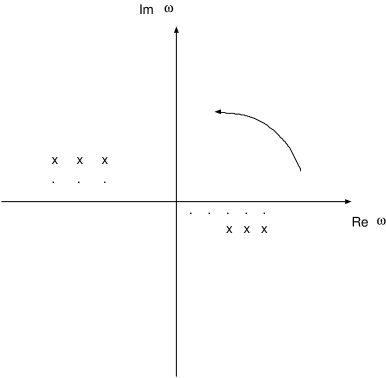
FIG. 7.: Rotation of the integration contour over $\omega$. The points indicate the positions of Green function poles; the crosses denote the positions of the poles of the polarization operator.

FIG. 8.: Insertion of the hole-particle interaction into the second order correlation correction.

FIG. 9.: Hole-particle interaction in the polarization operator.

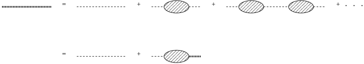
FIG. 10.: Renormalization of the Coulomb line due to the hole-particle interaction and screening.

FIG. 11.: The electron self-energy operator with screening and hole-particle interaction included.

FIG. 12.: Chaining of the self-energy operator.

FIG. 13.: Third-order diagrams of the interaction of a hole and particle from the loop with an external electron.

FIG. 14.: Correlation corrections to occupied orbitals of closed shells.

FIG. 15.: External field (denoted by a cross) in the external electron lines.

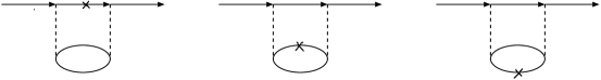
FIG. 16.: Structural radiation in diagram 2(a) of the self-energy operator.

FIG. 17.: Lowest order many-body perturbation corrections to the exchange potential; the cross denotes the external field.

FIG. 18.: Brueckner-type correlation corrections to the PNC E1 transition amplitude in first order in the weak interaction; the crosses denote the weak interaction and the dashed lines denote the electromagnetic interaction.

FIG. 19.: External field inside the correlation potential. In diagrams (a) the weak interaction is inside the correlation potential ($\delta\Sigma$ denotes the change in $\Sigma$ due to the weak interaction); this is known as the weak correlation potential. Diagrams (b,c) represent the structural radiation (photon field inside the correlation potential). In diagram (b) the weak interaction occurs in the external lines; in diagram (c) the weak interaction is included in the electromagnetic vertex.

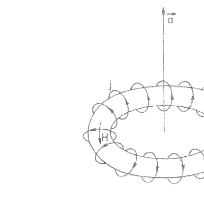
FIG. 20.: Diagram showing the anapole moment, ${\bf a}$, the toroidal current that produces it, ${\bf j}$, and the magnetic field that the current creates, ${\bf H}$.

FIG. 21.: Diagram showing the spin helix that occurs due to the parity violating nucleon-nucleus interaction. The degree of spin rotation is proportional to the distance from the origin and the strength of the weak interaction.

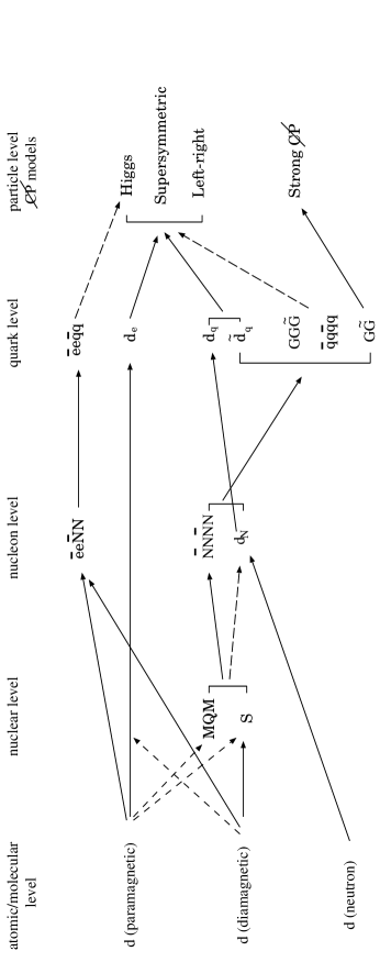
FIG. 22.: Flow diagram of CP-violation mechanisms at different levels that induce neutron, atomic, and molecular EDMs.

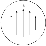
FIG. 23.: Constant electric field ${\bf E}$ inside the nucleus produced by the $P,T$-odd interaction (Schiff moment field). ${\bf E}$ is directed along the nuclear spin ${\bf I}$.