Diagrammatic Computation of the Random Flight Motion

Abstract

We present a perturbation theory by extending a prescription due to Feynman for computing the probability density function for the random flight motion. The method can be applied to a wide variety of otherwise difficult circumstances. The series for the exact moments, if not the distribution itself, for many important cases can be summed for arbitrary times. As expected, the behavior at early time regime, for the sample processes considered, deviate significantly from diffusion theory; a fact with important consequences in various applications such as financial physics. A half dozen sample problems are solved starting with one posed by Feynman who originally solved it only to first order. Another illustrative case is found to be a physically more plausible substitute for both the Uhlenbeck-Ornstein and the Wiener processes. The remaining cases we’ve solved are useful for applications in regime-switching and isotropic scattering of light in turbid media. It is demonstrated that under isotropic random flight with invariant-speed, the description of motion in higher dimensions is recursively related to either the one or two dimensional movement. Also for this motion, we show that the solution heretofore presumed correct in one dimension, applies only to the case we’ve named the ”Shooting Gallery” problem; a special case of the full problem. A new class of functions dubbed “Damped-exponential-integrals” are also identified.

1 introduction

The understanding of Brownian-motion has been of fundamental import on many levels in pure and applied physics. For example, the propagation of light in gaseous media has long been important in atmospheric and stellar physicsChandra . In chemical-physics the topology of polymerskleinert is of great interest. Yet, unlike topics of comparable ubiquity, Brownian-motion has immediate applications in the human realm, ranging from the physics of financeOsborne ; PhysicaA_v269 , to medical imagingOptTomo , to name only a very few.

The diversity of the applicants has resulted in a plethora of methodologies delineating the evolution of this ubiquitous topic. Among these techniques, the path integral formulation of the stochastic movement, while often more imaginative, is fairly under-represented. Meanwhile, the standard methodologies based on differential equations, often lead to difficult and unintuitive equations as soon as one gets away from the limiting situations such as infinitesimal mean-free-paths, or long-time regimes.

For example, the propagation of light through a stochastic medium is traditionally described in the context of astrophysics by a Boltzmann transport equation for the distribution of intensity $I(\textbf{r},\Omega,t)$ in a heuristic Radiative transfer theory Chandra2 . However,since the general analytic solutions are unknown, one resorts to the diffusion approximation which can be shown to arise out of the Radiative transport equation in the limit of large length scales $X\!>>\!L_{0}$, where $L_{0}$ is the transport mean-free-path of light in the mediumChandra2 ; Ishimaru .

In this same vein, there is considerable interest in the description of multiple light scattering at small length scales ($X\!\sim\!L_{0}$) and small time scales $\lambda T\!\sim\!1$ where $1/\lambda$ is the transport mean free time, both from the point of fundamental physics Kop , and from the point of many applications such as medical imaging, etc. Colak ; Wang . It has been experimentally shown that the diffusion approximation fails to describe phenomena at time scales where $\lambda T\!\lesssim\!10$ Yoo . Moreover the diffusion approximation, which is strictly a Wiener process, for the spatial coordinates of a particle is physically unrealistic. It holds only in the limit of the mean free path $L_{0}\!\rightarrow\!0$ and/or $\lambda\rightarrow\infty$ or the speed of propagation $c\!\rightarrow\!\infty$, while keeping the diffusion coefficient ($D\sim c^{2}/\lambda$) constant.

It is somewhat surprising that developing better alternatives to the diffusion approximation has had to wait until the 1990’s. For a particle moving with invariant speed in a one-dimensional disordered medium, it has been known for decades that the probability distribution function $P(X,T)$ for the displacement satisfies the telegrapher equation exactlyGoldstein . However, generalizations of the telegrapher equation to higher dimensions Durian have been shown not to yield better results than the diffusion approximation Porra ; Paasschens . Indeed we shall show (in section VI) that even the forementioned one-dimensional exact solution does not fully describe isotropic scattering, and additional diagrams are necessary to allow true isotropy. For a concise account of the recent work in light scattering work see Hindus .

In a similar mooring is the description of price movements in openly traded markets, where the diffusion approximation has been taken as gospel since the inception of theoretical finance. Meanwhile it has been known for over a centuryPareto that the actual probability distributions of the market prices deviate significantly from those expected based on the diffusive (Wiener) processes. More directly, there has never been any concrete empirical reasons to believe a property such as $\lambda\!\rightarrow\!\infty$ holds for the movement of openly traded market prices. With $\lambda\!\sim\!10^{21}/sec$ for the typical gasses which concerned the developers of the early physics literatureChandra , the approximation was more than adequate. On the surface it appears that this notion was taken from physics without proper care to ask if the underlying assumptions are satisfied in the movement of market prices. We submit that addressing this “misapplication” is well overdue. The recent wave of exploratory work on the notion of “regime switching” MarkovSrch ; Veronesi displays the burgeoning dissatisfaction with the gospel of diffusion in econophysics in general.

Elegant prescriptions for the solution of the Fokker-Planck equation exist with Kleinert3 and without Risken ; Martin resort to path-integral techniques which address the problem of classical stochastic probability density functions for arbitrary parameters and time scales. However, techniques generally become cumbersome when applied to motion not prescribed by analytic equations. Alas, many problems, particularly outside the realm of physical systems, involve discrete and/or non-smooth motion which are easy enough to conceive but not easily expressed analytically. The method we outline is arguably better suited for this type of problem than other, more sophisticated, theories.

In this report we present a technique based on a method invented by FeynmanFeynPIBook , allowing notions of Feynman diagrams for the random-flight movement. The technique of path integrationWiener , also known as sum over histories, is particularly attractive in the case of discrete stochastic motion because of the vivid imagery it evokes, literally illustrating the mathematical processpapadop .

In section-2 we summarize the groundwork on which we will build our method. In section-3 we present the full solution to an illustrative problem set up by FeynmanFeynPIBook but only solved for small displacements. Section-4 illustrates how extraneous features such as noise or force fields can easily be integrated in the “propagator”. As the final practice problem, section-5 presents the solution of an important variation on the problem of section-3. This variant can be considered a microscopically plausible alternative to the UhlenBeck-Ornstein process. The ensuing two sections, consider the problem of random flights under invariant speed, where the majority of the results presented are novel. We then conclude with two specific applications of selected results in modelling flexible (polymer) chains and stock prices.

2 Feynman’s prescription for stochastic processes

In this section we review the prescriptionFeynPIBook for computing the probability density function for a random process using functional integrals. Suppose that $f(t)$ describes a realization of a random process as function of time. Called a “probability functional”, $P[f(t)]$, then gives the probability density of a given realization. If we think of $f(t)$ as an ordered collection of discrete values $f_{1},f_{2},...,f_{n}$ in the limit of $n\!\!\rightarrow\!\!\infty$, the probability of finding a realization $f(t)$ is given by $P[f(t)]\mathcal{D}f(t)\equiv\lim_{n\rightarrow\infty}P(f_{1})P(f_{2})...P(f_{n})df_{1}df_{2}..df_{n}$ within a hyper-neighborhood given by the latter expression. The conjugate “characteristic functional” is computed by:

$$\Phi[k(t)]\equiv\frac{\int{e^{i\!\int{k(t)f(t)dt}}}P[f(t)]\mathcal{D}f(t)}{\int P[f(t)]\mathcal{D}f(t)}.$$ (1)

FeynmanFeynPIBook showed that despite the challenging appearance of this expression, it might be possible that under certain practical conditions the discretized form of $P[f(t)]\mathcal{D}f(t)$ can yield to either term by term integration, or known forms of path-integrals. Suppose that each random event has a time signature given by $g(t)$. Then the full realization of $n$-events over a fixed time interval $T$ is simply $f(t)=\sum_{j\,=1}^{n}g(t-t_{j})$. If the events are random and uniformly distributed in time, then the probability of each event occurring within the interval $dt$ is $dt/T$. Inserting $f(t)$ and $P[f(t)]$ into Eq.(1) and noting the identical form of each integral we get:

$$\Phi_{ng}[k(t)]=\int_{0}^{T}\exp{\left[i\sum_{j\,=1}^{n}\int k(t)g(t-t_{j})dt\right]}\;\;\frac{dt_{1}}{T}\ldots\frac{dt_{n}}{T}$$ (2)

$$\;\;\;\;\;\;\;\;\;\;\;\;\;=\left(\int_{0}^{T}e^{i\!\int k(t)g(t-\tau)dt}\frac{d\tau}{T}\right)^{n}.$$

where we have used $\tau$ as a stand in for any given $t_{j}$. For typical applications, the shape or at-least the amplitude of each event is often not fixed. We therefore consider the case $g(t)\equiv au(t)$ where the shape $u(t)$ of the event is fixed but its amplitude $a$ varies according to some probability density $p(a)$. We must now average $\Phi_{ng}[k(t)]$ over all values of $a$. Being that the latter is of form $(\phi_{g}[k(t)])^{n}$, and that the events are independently distributed, we can carry out this average over all g’s separately for each component $\phi_{g}$:

$$\phi\equiv<\!\phi_{g}\!>_{g}=\!\int_{0}^{T}\!\frac{d\tau}{T}\!\!\int\exp{\left[ia\!\!\int\!k(t)u(t-\tau)dt\right]}p(a)da.$$ (3)

Observe that the inner expression is a fourier transform of $p(a)$ where the frequency variable is the integral in the exponent. The fourier-transform being a characteristic-function, will be designated as $W[\int k(t)u(t-\tau)dt]$. Finally, if the number of events over $T$ is governed by a Poisson distribution, we can readily average over all possibilities of $n$:

$$\Phi[k(t)]=\sum_{n}\phi^{n}\frac{\bar{n}^{n}}{n!}e^{-\bar{n}}.$$ (4)

Here $\bar{n}=\lambda T$ is the average number of events expected over $T$. The sum is simply an exponential:

$$\Phi[k(t)]=e^{-(1-\phi)\bar{n}}=$$ (5)

exp [-λ∫_0^T( 1- W​​[∫k(t)u(t-τ)dt])dτ]. An important special case of the process described by Eq.(5) is when the signal-event has an extremely short duration in time: $u(t)=\delta(t)$. Then the characteristic functional becomes:

$$\Phi[k(t)]=\exp{\left[-\lambda\int_{0}^{T}(1-W[k(\tau)])\,d\tau\right]}.$$ (6)

3 The Gaussian Scattering Process

Using the characteristic Eq.(6) we can compute various moments of the signal profile $f(t)$. However, the true utility of this approach is to discover the resulting distributions of dependent variables which are driven by the events in $f(t)$. In this, and the following two sections, we will investigate cases of movement of free particles of unit mass, which undergo a prescribed change in their velocity for every event in $f(t)$. Initially the particles have a delta-function distribution in both speed and spatial spread. In between events, the movement of the particle is governed by its appropriate equation of motion. Our objective is to find the resulting spatial distribution of particles after a given time $T$.

At every event the particle acquires a change in momentum which is a random selection from a gaussian distribution of spread $s$ and zero mean. The characteristic function $W(\omega)$ of the gaussian random force-function profile is simply another gaussian. When inserted into Eq.(6) we have:

$$\Phi[k(t)]=e^{-\lambda T}\exp{\left[\lambda\int_{0}^{T}e^{-k(t)^{2}s^{2}/2}dt\right]}.$$ (7)

As discussed in the previous section, the probability density of the force function $P[f(t)]$ is given by the fourier transform of $\Phi[k(t)]$, as given by Eq(1):

$$\!\!\!\!\!\!\!\!\!\!\!\!P[f(t)]\!=\!\int\!\!\Phi[k(t)]e^{-i\int k(u)f(u)du}\mathcal{D}k=e^{-\lambda T}\!\!\!\int\!\!e^{\lambda\int_{0}^{T}e^{\!-k(t)^{2}s^{2}/2}dt}e^{-i\int_{0}^{T}\!k(u)f(u)du}\mathcal{D}k$$ (8)

In order to proceed, we discretize the time interval $[0,T]$ into $N$, regular small intervals of duration $\eta$. With the understanding that $N\!\!\rightarrow\!\infty$ we can write:

$$P[f_{i}]=e^{-\lambda T}\prod_{i}^{N}\int\frac{dk_{i}}{2\pi}\exp{\left[\lambda\eta e^{{-k_{i}}^{2}s^{2}/2}\right]}e^{-i\eta k_{i}f_{i}}.$$ (9)

Finally, we expand the first exponential in a Taylor series and carry out the individual fourier transforms:

$$P[f_{i}]=e^{-\lambda T}\prod_{i}^{N}\left[\delta(f_{i}\eta)+\frac{\lambda\eta}{s\sqrt{2\pi}}e^{-{(f_{i}\eta)}^{2}/2s^{2}}+\ldots\right]$$ (10)

whereupon we recognize $f_{i}\eta\equiv I_{i}$ as the impulse imparted at time $t_{i}$. The leading (zeroth-)order in $\eta$ is a product of $\delta$-functions which we’ll call a $\delta$-functional $\delta[I(t)]$. The value of the functional is zero unless the function $I(t)$ is zero for all $t$. The zeroth-order term

$$P_{0}[I(t)]=\delta[I(t)]$$ (11)

corresponds to the ballistic path where the particle experiences no collisions and hence experiences no impulses. The $O(\eta)$ terms are comprised of all $\delta$’s, except at time $t_{i}$ where a single term of $O(\eta)$ contributes. There are $N$ such terms (one for each $t_{i}$) comprising a Riemann sum. In the limit of large $N$ this sum becomes the integral:

$$P_{1}[I(t)]=\frac{1}{s\sqrt{2\pi}}\int_{0}^{T}dt\;e^{-{I(t)}^{2}/2s^{2}}\bar{\delta}[I(t)].$$ (12)

The functional $\bar{\delta}[I(t)]$ is defined as the ($\lim_{N\rightarrow\infty}$) product of $\delta(I(t_{i}))$ for all $t_{i}$ except $t_{i}=t$. This term describes the path where there is only a single collision at time $t$. It is easy to show that if the scattering profile had an offset, then it would change the exponent of the integrand to $I(t)-I_{0}$. Higher order terms in $\eta$ are easily obtained:

$$P_{n}[I(t)]=\prod_{i=1}^{n}\frac{1}{{s\sqrt{2\pi}}}\int_{0}^{t_{i+\!1}}dt_{i}e^{-{I(t_{i})}^{2}/2s^{2}}\bar{\delta}[I(t_{1}),...,I(t_{n})]$$ (13)

where $t_{n+1}\equiv T$. Upon collecting the orders we get the expression for the probability density functional of Eq(10):

$$P[I(t)]=e^{-\lambda T}\sum_{n=0}^{\infty}\lambda^{n}P_{n}[I(t)].$$ (14)

In order to obtain the probability density of a given output position $P(X)$ we must first derive $P[x(t)]$ from $P[I(t)]$. We then will sum over all paths $x(t)$ which satisfy the boundary conditions: $x(t=0)=x_{0}$ ; $x(t=T)\equiv X$; $\dot{x}(t=0)=v_{0};\dot{x}(t=T)=V$.

The final sum over paths can easily be done because of the insight we have acquired by recognizing the various orders in the series of Eq.(14) as paths with a given number of events. The zeroth order term is the easiest; it is simply the sum over all paths which experience no impulses, of which there is only one. However, to proceed more formally we will utilize the following observationFeynPIBook . As long as the relation between $I$ and $x$ is linear (e.g. $I\propto\ddot{x}$), we can be sure that any Jacobian resulting from the change of variable:

$$P_{n}[I(t)]\mathcal{D}I=P_{n}[x(t)]\mathcal{D}x$$ (15)

is a constant, and if skipped, affects only the normalization of the final answer. The normalization of the resultant distribution must be ensured regardless. Thus, from Eq.(13), and (15):

$$P_{0}(X,T)=\int\delta[I(t)]\mathcal{D}I=\int\delta[\ddot{x}(t)]\mathcal{D}x=\delta(X\!-v_{0}T).$$ (16)

The above relation (arguably the easiest path integral known) establishes the “propagator” for the process. Using Eqs.(13), (15), and two applications of Eq.(16), the first order term is the sum over all paths with a single event and is given by:

$$P_{1}(X,T)=\frac{1}{s\sqrt{2\pi}}\int_{0}^{T}dt_{1}\int_{-\infty}^{+\infty}dx_{1}\int_{-\infty}^{+\infty}dI_{1}$$ (17)

$$\;\;\;\;\;\;\;\;\;\;\times\;\;\delta\left(X-\left((v_{0}+I_{1})(T-t_{1})+x_{1}\right)\right)e^{-I_{1}^{2}/{2s^{2}}}\delta(x_{1}-v_{0}t_{1}-x_{0}).$$

This expression is easy enough to evaluate using the rule $\delta(ax)=\delta(x)/|a|$ and we will do so shortly.

3.1 Feynman Rules

Upon writing the sequence of terms $P_{1},P_{2},...$ we can see the that the unevaluated integrals (such as Eq.(17)) can be represented by diagrams. The diagrams comprise propagators, interaction points and the necessary factors to integrate over intermediate variables. In one-dimension the $n^{th}$ term is given by:

$$P_{n}(X,T)=\int d^{2}x_{n}\ldots\int d^{2}x_{1}K_{fn}V_{n}\ldots K_{21}V_{1}K_{1i}$$ (18)

where $\int d^{2}x_{i}=\int_{-\infty}^{\infty}dx_{i}\int_{0}^{t_{i+\!1}}dt_{i}$. The specifics of the problem are contained in the propagator $K$ and the interaction profile $V$. Each term in the above equation, and the final summation thereof can be represented diagrammatically as in figure-1.

For the case of a free particle undergoing a scattering process (which conserves momentum), the propagator is:

$$K_{i+\!1,i}^{s}=\frac{1}{t_{i+\!1}\!-t_{i}}\!\!\int_{-\infty}^{+\infty}\!dI_{i}\,\delta\!\!\left(I_{i}-(\frac{x_{i+\!1}-x_{i}}{t_{i+\!1}-t_{i}}-\!\!\sum_{k=1}^{i}I_{k}-v_{0})\!\!\right)\!.$$ (19)

(Note: we will only treat the case of free particles here, so we will not clutter the super/subscript notation to that effect.) The interaction points $V^{g}_{i}\!=\frac{1}{\sqrt{2\pi s^{2}}}e^{I^{2}_{i}/2s^{2}}$ contain the gaussian profile of the $i^{th}$ event.

The propagator can be generalized to other types of motion between collisions by simply replacing the classical equation of motion as the argument of the $\delta$-function or other appropriate kernel.

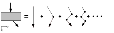
Figure 1: The diagrammatic representation of brownian motion through a medium.

At higher orders, the computation gets increasingly difficult and a recursion relation between orders of $P_{n}$ does not exist in general. This is true in the present case of gs-process. For example to get $P_{3}^{gs}$ we must repeat the integration over $x_{2}$ because $K^{s}_{f3}$ involves $x_{2}$. Therefore a more complicated integral over $x_{2}$ must be performed before the integration over $x_{3}$ is done. Despite this complication, the computation of $P_{n}^{gs}(X,T)$ can be carried out for arbitrary $n$, giving:

$$P_{n}^{gs}(X,T)=\frac{1}{\sqrt{2\pi}}\int_{0}^{\;\;\;T}dt_{n}\ldots\int_{0}^{\;\;\;t_{2}}dt_{1}\frac{1}{\xi_{n}^{gs}}\exp{\left(-\frac{(x-(x_{0}+v_{0}T))^{2}}{2\,{\xi_{n}^{gs}}^{2}}\right)}$$ (20)

where the “interim variance” ${\xi_{n}^{gs}}^{2}$, is given by:

$${\xi_{n}^{gs}}^{2}=s^{2}\sum_{i=1}^{n}(T-t_{i})^{2}.$$ (21)

As we will see below, the summation over the orders can be easily carried out in the fourier domain.

Should for some reason, the effect of scattering medium be artificially stopped after a fixed number of events, then the probability distribution is given by a new class of functions which we have named: “Damped exponential integrals”. These functions are described in the appendix-A.

3.2 Normalization

We can directly demonstrate the normalization of $P^{gs}(X,T)$ by integrating Eq.(20) over all $X$, and inserting the resulting terms in Eq.(14). Moreover, it is interesting to note the temporal population of each “generation” is:

$$N_{n}(T)=\frac{e^{-\lambda T}\lambda^{n}}{n!}\int P_{n}(X,T)dX=\frac{(\lambda T)^{n}}{n!}e^{-\lambda T}.$$ (22)

Reflecting our initial assumption, this is simply the Poisson distribution. Summing over all $n$ shows normalization. The population of generation $n$ will rise and fall according to the above relation each with a peak at $T=\lambda/n$ (figure-2).

Figure 2: The relative population Eq.(22) of generations $n$, being the number of events they have experienced. Curves shown here are for $\lambda=0.1$. The peaks occur at $T=\lambda/n$.

Another way to verify the normalization of the gaussian-scatter solution is as follows. The quantities $N_{n}(T)$ must satisfy the simple coupled rate equations:

$$\dot{N_{0}}=-\lambda N_{0}$$ (23)

$$\dot{N_{1}}=\lambda N_{0}-\lambda N_{1}$$

$$\ldots$$

$$\dot{N_{n}}=\lambda N_{n-1}-\lambda N_{n}.$$

It easily verified that the solution for these equations is given by Eq.(22)

3.3 Moments and Kurtosis

We will shortly demonstrate that the exact characteristic function for the gs-process $\Phi_{gs}(k,T)$ can be obtained. Therefore all moments can be readily obtained by simple differentiation. However, the ability to obtain the characteristic function for a given process in closed form is not guaranteed. Hence we will demonstrate the direct computation of the moments by summing the moments of each order. We shall specialize to the case where all initial settings $x_{0},v_{0},I_{0}$ are zero. we compute The $m^{th}$ moment of the $n^{th}$ order distribution and then sum them according to Eq.(14). For the second moment this is:

$$<\!X^{2}\!\!>^{gs}_{n}=\frac{s^{2}}{n!}\int_{0}^{T}\ldots\int^{T}_{0}d^{n}\tau\sum_{i=1}^{n}\tau^{2}_{i}=\frac{s^{2}T^{n+2}}{3(n-1)!}$$ (24)

where $\tau_{i}=(T-t_{i})$. The discrete sum is $n\tau^{2}$ by symmetry. The integral on $\tau^{2}$ is simply $T^{3}/3$ and the remaining $n-1$ integrals of measure unity give $T^{n-1}$. Inserting the result in Eq.(14) gives:

$$\nu_{gs}\equiv<\!X^{2}\!\!>_{gs}=\frac{1}{3}s^{2}T^{2}e^{-\lambda T}\sum_{n=1}^{\infty}\frac{(\lambda T)^{n}}{(n-1)!}=\frac{1}{3}s^{2}\lambda T^{3},$$ (25)

in agreement with the first order computation in FeynPIBook .

Based on the statement of the problem we can expect $<\!V^{2}\!\!>\propto s^{2}T$. Traditionally the computation of Brownian motion is within a system in equilibrium with a well defined temperature. In that case Chandra ; papadop the thermal equilibrium constrains the parameter $s$ to the coefficient of friction and the temperature, and all three to $<\!V^{2}\!\!>$. In the present case, no friction exists, therefore nor a finite temperature as evidenced by the ever increasing $<\!V^{2}\!\!>$. The cubic dependence of the variance on observation time is reminiscent of the diffusion of tracer particles in turbulent flows. Richardsonrichardson was able to produce such a behavior for in the context of continuous diffusion only using a diffusion coefficient which depends on position as $R^{4/3}$ (alternatively a time dependence of form $T^{2}$ could also do itShlesingerPhysToday ). More recently, it has been shownShlesingerPRL87 that a Levy-distribution of waiting times can obviate the need for a space or time dependent diffusion coefficient in getting several families of supra-linear variances, one of which includes $T^{3}$. The above result shows that a Poisson distribution can also give $T^{3}$ for the variance.

A similar but more tedious computation for the fourth moment produces:

$$\chi_{gs}\equiv<\!X^{4}\!\!>_{gs}=s^{4}\lambda T^{5}(\frac{3}{5}+\frac{\lambda T}{3}).$$ (26)

The first term is the result of cross-terms like $(T-t_{i})^{2}(T-t_{j})^{2}$ in the time integrals, whereas the second term is the result of direct-terms like$(T-t_{i})^{4}$. Ostensibly, it is the presence of the interference terms that cause deviations from a normal distribution. Although as expected (from the central-limit-theorem) the deviation is transient. To quantify this, we compute the kurtosis for the process:

$$\kappa_{gs}\equiv\frac{\chi_{gs}}{3{\nu_{gs}}^{2}}-1=\frac{9}{5\lambda T}.$$ (27)

Thus the distribution approaches normality in time. It is, moreover, worth noting that this result is independent of the parameter $s$.

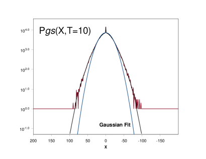
Figure 3: Demonstration of The Kurtosis(Fat-tails) as calculated for the gs-process at $\lambda T=10$ versus the computer simulation of the gs-process (The noisy line). The fit of the latter to a normal distribution is also shown. As expected from the central-limit theorem, the fit to a normal distribution progresses over time from the peak to the tails. Unlike the exact solution, the ballistic peak is not present in the normal distribution.

3.4 The Characteristic Function

Having arrived at a solution for $P_{n}^{gs}(X,T)$ (Eq(20)), the characteristic function is easily found by exploiting the symmetry in $\xi^{gs}$ in the fourier transform of each $P_{n}^{gs}$. The symmetry allows us to convert the sequence of connected integrals into the $n^{th}$ power of a single integral from 0 to $T$ with an added $1/n!$ pre-factor. We can then sum them according to Eq.(14). The result is:

$$\Phi_{gs}(k,T)=e^{-\lambda T}\exp{\left(\sqrt{\frac{\pi}{2}}\frac{\lambda}{ks}\>E\!r\!f\!\!\left(\frac{ksT}{\sqrt{2}}\right)\right)}.$$ (28)

Both the second and fourth moments can readily be verified by repeated differentiation of $\Phi_{gs}(k,T)$ with respect to $k$. The distribution $P_{gs}(X,T)$ is shown in figures-3 and 4 versus a computer simulation.

Figure 4: $P_{gs}(X,T)$ as calculated by a numerical simulation of the gs-process. The one-dimensional distribution is shown at different observation times $T$. For comparison, at the corresponding time, the prediction of the theory (numeric inverse transform Eq.(28)) is superposed on the widest distribution. Only the amplitude of the theoretical curve has been adjusted to match the simulation. The spike at $X=0$ is the ballistic peak corresponding to the zeroth order theory (not shown).

If it should happen that the deterministic equation of motion of the projectile is of the general type, $x(t)\propto v_{0}t^{\alpha}(0<\alpha\leq 1)$, then the result is a simple redefinition of Eq.(21) and for certain rational values of $\alpha$ the characteristic function can be easily computed. The result is that the variance will be proportional to $T^{1+2\alpha}$ and fourth moment will be such that the kurtosis remains proportional to $1/T$, independently of both $\alpha$ and $s$. This is consistent with the Central Limit Theorem.

3.5 Higher Dimensions

For the case of a homogeneous and isotropic medium, and where the scattering profile has no preferred axis, it is easy to verify starting from the fundamentals of the theory, that the answer is found by replacing the scalar wave-number $k$, with the magnitude of the wave-vector. In case such rotational symmetry exists, by applying the inverse fourier transform we arrive at the probability density integrated over a D-dimensional spherical shell at $R$:

$$P(R)=\frac{R}{(2\pi R)^{D/2}}\int_{0}^{\infty}\!\!J(D\!/2-1,kR)\;\Phi(k)\;k^{D\!/2}dk.$$ (29)

where, $R=|\mathbf{X}|$, and $J(D\!/2-1,kR)$ is the Bessel function of the first kind and of order $(D\!/2\!-\!\!1)$. Thus, if the gs-process is applicable, we can insert the $D^{th}$ power of the characteristic function $\Phi_{gs}$ directly into the above relation.

Alas the gs-process is not applicable to photons because the postulate of relativity is not satisfied by the infinite tail of the Gaussian interaction kernel and the change in momentum after each scattering event is not independent of those along other dimensions. We will treat such constrained interactions separately.

4 The Effect Of Noise

If it should be that instead of simple traversal of the medium the particle diffuses in between collisions (“noisy paths”). We can show that insight provided by the imagery of paths allows us to see our way through this added effect. Suppose $P_{gsd}(y,T)$ is the probability density of arriving at $(y,T)$ when diffusion is present. arriving at position $y$ can proceed along an infinite number of paths which would have culminated at different $x$’s if diffusion were not present. If we let $y\!=\!x\!+\!z$ then $z$ is the component of motion due to noise. Thus the $P_{gsd}(y,T)$ is the sum of all pairs $(x,z)$ which satisfy the above constraint:

$$P_{gsd}(y,T)=\int\!\!dx\!\int\!\!dz\,P_{gs}(x,T)P_{d}(z,T)\delta(y-(x+z))$$ (30)

$$\;\;\;\;\;\;\;\;\;\;\;\;\;\;=\int\!\!dx\,P_{gs}(x,T)P_{d}(y-x,T).$$

From here it can be easily shown that the effect can wholly be incorporated into a new propagator $K^{sd}$. This is what we would have expected based on the previously alluded path imagery. The new propagator (itself obtainable by the path integral method wiegel ) is simply a broadened form of $K^{s}$

$$\!\!\!\!\!\!\!\!K_{i+1,i}^{sd}=\frac{1}{\sigma\sqrt{2\pi(t_{i+1}-t_{i})}}\int_{-\infty}^{+\infty}dI_{i}\exp{\left(-\frac{(I_{i}-(\frac{x_{i+1}-x_{i}}{t_{i+1}-t_{i}}-\sum_{k=1}^{i}I_{k}-v_{0}))^{2}}{2\sigma^{2}/(t_{i+1}-t_{i})}\right)}$$ (31)

where $\sigma^{2}$ is the diffusion coefficient. The computation of $P_{gsd}(y,T)$ proceeds as before. Computation will show that in presence of diffusive movement between scattering events, the diffusion acts in parallel to the process and thus simply adds a net term to the variance of the process. Thus, the “interim variance” is:

$${\xi_{n}^{gsd}}^{2}={\xi_{n}^{gs}}^{2}+\sigma^{2}T.$$ (32)

And we find for the full variance:

$$\nu_{gsd}\equiv<y^{2}>_{gsd}=\frac{1}{3}s^{2}\lambda T^{3}+\sigma^{2}T;$$ (33)

the fourth moment:

$$\!\chi_{gsd}\;\equiv\;<y^{4}>_{gsd}\;=\;s^{4}\lambda T^{5}(\frac{3}{5}+\frac{\lambda T}{3})+\sigma^{2}T^{2}(3\sigma^{2}+2s^{2}\lambda^{2}T^{2});$$ (34)

and the kurtosis:

$$\kappa_{gsd}=\frac{9s^{4}\lambda T}{5(\lambda s^{2}T^{2}+3\sigma^{2})^{2}}\,\,_{\overrightarrow{T_{large}}}\,\,\frac{9}{5\lambda T}.$$ (35)

We observe that over long times, the effect of diffusion (noise) becomes insignificant. Finally the characteristic function is found to be:

$$\Phi_{gsd}(k,T)=e^{-(\lambda+\sigma^{2}k^{2}/2)T}\exp{\left(\sqrt{\frac{\pi}{2}}\frac{\lambda}{ks}\>E\!r\!f\!\!\left(\frac{ksT}{\sqrt{2}}\right)\right)}.$$ (36)

In this section we have seen that diffusive intra-event movement can be represented by a change in the functional form of the propagator. Other effects such as that of an external force field can be added to the theory by incorporating the equation of motion in the argument of the propagator. For an absorptive medium, a damping factor in the propagator will be necessary.

5 The Gaussian Reset Process

Consider if instead of scattering, we characterize the events as “resets” in the particle’s momentum. It would be as if the previous momentum is lost at each event and a new one selected from a gaussian distribution of width $s$. This change implies only a different propagator:

$$K^{r}_{i+1,i}=\int\frac{dI_{n}}{t_{i+1}-t_{i}}\,\delta\!\!\left(I_{i}-\frac{x_{i+1}-x_{i}}{t_{i+1}-t_{i}}\right).$$ (37)

Utilizing this propagator in the Eq.(18), and other rules we find the probability density function $P^{gr}_{n}(X,T)$ to be the same form as the Eq.(20) if only we use a different “interim variance” function as given by:

$${\xi_{n}^{gr}}^{2}=s^{2}\sum_{i=1}^{n}(t_{i+1}-t_{i})^{2}.$$ (38)

Following the same steps as in the gs-process, we can show that in presence of diffusive movement between reset events the diffusion acts in parallel to the process and thus simply adds a net term to the “interim variance”:

$${\xi_{n}^{grd}}^{2}={\xi_{n}^{gr}}^{2}+\sigma^{2}T.$$ (39)

Unfortunately, for this process, ${\xi_{n}^{gr}}^{2}$ does not posses the symmetry which allowed us to compute the characteristic-function in closed form for the gs-process. Thus we must compute the various moments by summing the moments of each $P^{gr}_{n}(X,T)$ according to Eq.(14). This task, while a little tedious for higher moments, is straightforward. The variance is found to be:

$$\nu_{gr}\equiv<X^{2}>_{gr}=\frac{2s^{2}}{\lambda^{2}}\left(2(e^{-\lambda T}-1)+\lambda T(e^{-\lambda T}+1)\right).$$ (40)

In very early times the variance increases as $s^{2}\lambda T^{3}/3$ which matches $\nu_{gs}$. Later, the momentum non-conservation in this process manifests its different character resulting in slower spreading of the distribution. For this process the variance becomes linear in $T$ in the long time limit ($\lambda T\gg 1$).

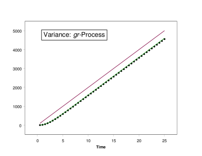
Figure 5: The comparison of the variance as calculated from a simulation of the gr-process (dots), compared to Eq.(40). The upper solid line is that of $2s^{2}T/\lambda$ which is the progression of variance in (Wiener process) applications such as in Black-Scholes options-valuation. At early times, the linear approximation grossly overestimates the gr-variance.

The fourth moment is:

$$\!\!\chi_{gr}\equiv<X^{4}>_{gr}$$ (41)

$$\;\;\;=\frac{4s^{4}}{\lambda^{4}}[e^{-\lambda T}(12+18\lambda T+9\lambda^{2}T^{2}+2\lambda^{3}T^{3})-12\;-6\lambda T+3\lambda^{2}T^{2}].$$

At early times, the fourth moment also behaves like $\chi_{gs}$ increasing proportionally to $T^{5}$, but later it settles into a parabolic increase. The kurtosis for the gr-process has a steep fall off at early times, but then it too settles into $\sim 1/\lambda T$ descent:

$$\kappa_{gr}\,\,{}_{\overrightarrow{T_{large}}}\;2\frac{\lambda T-4}{(\lambda T-2)^{2}}.$$ (42)

Observe that the eventual linearity of the variance is reminiscent of the Uhlenbeck-Ornstein (UO-)process (see e.g.Risken ,ch.3). The UO-process is random flights (i.e. the Wiener-process) in the presence of continuous friction. However, continuous friction may not be a plausible mechanism at the ”atomic” scale, where by an ”atom” we may mean: an atom of matter, a node on a network, an individual trader, etc. Hence it is tempting to to think of the gr-process as the microscopic alternative to the mesoscopic UO-process. As a reminder, both the UO and gr-processes approach the limit of the Wiener process, if we turn off friction in the former($\gamma\rightarrow 0$ but $\gamma\theta$ finite - as defined below), or allow very large number of collisions per unit time ($\lambda T\gg 1$) for the latter.

For the UO-process, in time, the variance approaches $\nu_{UO}=2\theta T/m\gamma$, where $\theta$ is the absolute temperature and $\gamma$ is the coefficient of friction. Thus to match this with the gr-process we must have: $\theta/m\gamma=s^{2}/\lambda$. if we arbitrarily set $\theta/m=s^{2}$, and $\gamma=\lambda$, then a graph of $\nu_{UO}$ looks quite a bit like that of $\nu_{gr}$ (fig-5). However, it is not possible to exactly match the variance of the UO-process to that of the gr-process for all times for any conceivable relation between ($s$,$\lambda$) and ($\theta$,$\gamma$). This stems from the fact that these parameters represent quite different physical meanings. Still it is interesting to note that (unlike the gs-process) the gr-process has an effective temperature due to the stabilizing effect of the reset mechanism which acts as as a form of friction. Thus the choice between the UO vs. gr-processes as the appropriate physical model for a given system lies with the end-user.

We conclude by stating the moral of this section. Even if the probability distribution (or its characteristic function) may not be computable in closed form, in many cases, our method allows access to the exact moments of the distribution.

6 The Shooting Gallery

To further demonstrate the versatility of this method we will take on a problem where a solution by the “traditional” approach of stochastic differential equations is difficult. Consider the carnival game of “Shooting Gallery”. A “target-duck” starts moving at the center of a plank with a fixed speed $c$ to the right. The player is required to shoot the duck. On every hit the duck reverses direction and continues to retrace its path with speed $c$. After a time $T$, we need to know the probability distribution of finding the duck at a given position $X$ within $dX$. As before, the number of shots is given by the Poisson distribution of mean $\lambda T$, but otherwise uniformly distributed over [0,T].

The scattering profile (i.e. the distribution from which the next momentum change is selected) is now comprised of two $\delta$-functions, each offset by the amount $\pm c$, respectively. Each lobe of the scattering profile is used in alternate order. The alternation requirement is an instance of a situation where the description of the motion does not lend itself well to analytic description. Because there is a binary alternation between left-right symmetric profiles we will call this process the “symmetric-binary-delta-scattering”, or sbds-process.

The propagator for this problem is the same as that of gs-process (Eq.(19)). Furthermore the result for the $P_{1}^{gs}$ when $v_{0}\neq 0$ (Eq(17)) applies if we replace the interaction kernel (gaussian profile) with $\delta(I_{1}+2c)$. Higher orders can easily be written using the Feynman-rules for this case. Integration over intermediate positions can proceed as before and the analog to of Eq(20) is found to be:

$$\!\!\!\!\!P_{n}^{sbds}(X,T)=\int_{0}^{T}dt_{n}\ldots\int_{0}^{\;\;\;t_{2}}dt_{1}\delta\!\left(X-(v_{0}-c)T-c\sum_{i=0}^{n}(-1)^{n}(t_{i+1}-t_{i})\right)$$ (43)

where $t_{0}=0$, and $t_{n+1}=T$. We consider only the initial condition $v_{0}=c$ which results in cancellation the second term. Although higher orders of the above integral require a good bit of bookkeeping, the actual integration are straightforward if aided by computer. By extensive use of the rule, $\int_{a}^{b}d\tau\delta(\!\tau-t)f(\tau)=f(t)[\Theta(b\!-t)-\Theta(a\!-t)],$ we find $P_{n}^{sbds}(X,T)$ to be:

$$\delta(X-cT)\;\;\;\;\;\;\;\;\;\;\;\;\;\;\;\;n=0;$$

$$\frac{(c^{2}T^{2}-X^{2})^{\frac{n-1}{2}}}{2\;c^{n}\;(n-1)!!^{2}}\;B(X,cT)\;\;\;\;n=1,3,5,...;$$

$$\frac{(X+c\;T)(c^{2}T^{2}-X^{2})^{\frac{n-2}{2}}}{2\;c^{n}\;n!!\;(n-2)!!}\;B(X,cT)\;\;\;\;n=2,4,6,...;$$

where $n!!\!=\!(n/2)!\,2^{n/2}$ ($n$-even, e.g. $6!!=6\cdot 4\cdot 2$). The “light cone” is maintained by the “box-car” function: $B(X,cT)=\Theta(X+cT)-\Theta(X-cT)$. Finally, the observed probability density is found by summing $P_{n}^{sbds}$ according to Eq.(14). To aid the summation process we can shift the dummy index $n\rightarrow 2n+2$ for even terms and $n\rightarrow 2n+1$ for the odds. The summed result is:

$$\!\!\!\!\!\!\!\!\!\!P_{\!sbds}(X,T)=e^{-\lambda T}\!\left(\delta(X-cT)+\frac{B(X,cT)}{2c/\lambda}\left[\frac{(X+cT)}{\rho c/\lambda}I(1,\rho)+I(0,\rho)\right]\right)$$ (45)

where $I(k,\rho)$ is the modified Bessel function of the first kind and of order $k$. $\rho$ is a measure of position within the light-cone, given by:

$$\rho\equiv\left(\frac{c^{2}T^{2}-X^{2}}{(c/\lambda)^{2}}\right)^{1/2}$$ (46)

We note that this is in agreement with Goldstein derived by a laborious solution to a coupled set of “telegrapher’s equations”. Figure-6 shows samples of $P_{sbds}$ over a relatively early time range for $\lambda=1$ and $c=1$.

Figure 6: The time evolution of the sbds-process for $c=1,\lambda=1$. Here The zeroth order ($\delta(\!X-\!cT)$ in Eq.(45)) ballistic peaks have been artificially broadened for plotting.

The solution above and that in the figure pertain to the initial condition: $P(\!v_{0}\!=\!c)\!\!=\!\!1$. In the event $P(v_{0}\!=\!-c)\!\neq\!0$ then the solution can easily be constructed by the superposition $P(v_{0}\!=\!c)P_{sbds}(X,T)+P(v_{0}\!=\!-c)P_{sbds}(-X,T)$.

Finally, we could have modelled the problem with a reset type propagator as in Eq(37). It is easy to show that the resulting sbdr-process will give the same answer as long as the initial condition $v_{0}=\pm c$ applies, but not otherwise.

7 Isotropic Random Flight in $D$-dimensions at an Invariant Speed

Extending the previous section’s model to higher dimensions is of great practical interest in physical systems. Our method facilitates the setup without difficulty. We shall denote the unit vector along the $d^{th}$ component of motion after the $j^{th}$ scattering event as $e_{jd}$. As before, we assume that the particle moves at a constant speed $c$, and use the propagator of Eq.(19) for a free, momentum-conserving particle. After the easy integration over intermediate positions we obtain for the end-to-end propagator of the $d^{th}$ component of the position:

$$\delta\!\left(R_{d}-(v_{0d}-ce_{0d})T-c\sum_{j\,=0}^{N}e_{jd}(t_{j\,+1}-t_{j})\right)$$ (47)

where $t_{0}=0$, and $t_{N+1}=T$. The above integrand is quite plain in its statement about the free particle, and could have been written without the need for integration over many intermediate coordinates. We can consider two possible initial conditions: 1. An incident beam where $v_{0}=c$, or 2. A source emitter where $v_{0}=0$. In the former case we can select $\textbf{v}_{0}=c\textbf{e}_{0}$ resulting in cancelling the middle term, but we must maintain $\textbf{e}_{0}=(0,0,...,1)$. Alternatively, we can shift the sum to start from 1 but remember that the position vector is given by $\textbf{R}=(x,y,...,z-ct_{1})$. The latter case is simpler because we have $\textbf{e}_{0}=\textbf{0}$ which simply eliminates the middle term, the sum remains as is, and $\textbf{R}=(x,y,...,z)$. Either way, the computations do not depend on the absolute value of the index $j$, hence this distinction between initial conditions does not come into play until the very end whence integrating over interaction times.

According to the Feynman rules, we must now add the interaction kernels and sum over all allowable intermediate directions $e_{jd}$ as well as times $t_{j}$. The allowable states for the particle include only those which maintain a constant speed $c$. Therefore, for movement in Euclidean space, we must implement the constraint $\sum_{d=1}^{D}e_{jd}^{2}=1$ for all $j$. Thus the full diagram for the $N^{th}$ order for the D-dimensional scattering (Dds-)process is:

$$\!\!\!\!\!\!\!\!\!\!\!P_{ND}^{Dds}(X,T)=\prod_{j\,=0}^{N}\int_{0}^{t_{j\,+1}}\!dt_{j}\;\;\;\prod_{d=1}^{D}\!\int_{-\infty}^{\infty}de_{jd}$$ (48)

$$\;\;\;\;\;\;\;\;\;\;\;\times\;\;\;V(\textbf{e})\;\;\delta\!\left(R_{d}-c\sum_{j\,=0}^{N}e_{jd}(t_{j\,+1}-t_{j})\right)\delta\!\left(1-\sum_{d=1}^{D}e_{jd}^{2}\right).$$

As a consequence of the nonlinearity of the unit vector constraints, additional normalization factors will be needed depending on the explicit dimensionality. Here we will consider isotropic scattering and thus set $V(\textbf{e})=1$.

In performing these summations we employ a technique which could also apply to most of the problems we considered previously, but did not for the sake of illustration of the possibility of direct integration. The $\delta$-function can be represented as an unweighted superposition of plane waves. This action, amounting to a fourier transformation of the integrand, results in the computation of the characteristic function instead the probability density. However, in this case the decomposition is especially necessary. Once decomposed, terms involving a single $e_{jd}$ are collected and integrated separately. There is, however, one further complication: An integration over $e_{jd}$ diverges unless the wave number corresponding to the second $\delta$-function is always positive. For this reason we choose an alternate (if obscure) plane wave superposition given by, $\delta(x)=Re\left(\int_{0}^{\infty}e^{i\kappa x}d\kappa/\pi\right)\!-\!i/{\pi x}$, where the second term is understood as the principle value. Together with the ordinary decomposition of the first $\delta$-function, the integrals over $e_{id}$ involving terms like $i/{\pi x}$ will all vanish. The remainder of terms with $e_{jd}$ each result in $\sqrt{\pi/{i\kappa_{i}}}\exp{\left(ik_{d}^{2}c^{2}(t_{j\,+1}-t_{j})^{2}/4\kappa_{j}\right)}$ where the nested products over $j$ and $d$ apply. In order to carry out the integration over the $\kappa_{j}$ we perform the product over $j$. This conveniently results in the square of the magnitude of the $D$-vector k in the exponent. Thus we arrive at:

$$\phi_{D}(k,t_{j})=\frac{1}{\pi}\int_{0}^{\infty}\frac{e^{-\frac{s_{j}^{2}+\kappa_{j}^{2}}{i\kappa_{j}}}}{(i\kappa_{j}/\pi)^{D/2}}\;\;d\kappa_{j}$$ (49)

where, $s_{j}\equiv kc(t_{j\,+1}-t_{j})/2$ and $k=|\textbf{k}|$. Applying the product over $j$ to $Re(\phi_{D})$, and the integration over all interaction times $t_{j}$, we arrive at the characteristic function for the isotropic scattering after $N$-events:

$$\Phi_{N}^{Ddis}(k)=\prod_{j\,=0}^{N}\int_{0}^{t_{j\,+1}}Re(\phi_{D}(k,t_{j}))dt_{j}.$$ (50)

Before proceeding, we note an important property of $\phi_{D}$:

$$\phi_{D+2}=-\frac{1}{2s}\frac{\partial\phi_{D}}{\partial s}.$$ (51)

That is, the respective characteristic functions for all odd and separately, all even dimensions are recursively related. For this reason we need to evaluate the expression in Eq.(49) for $D$=1, and 2 only, viz.,

$$\phi_{1}(s)=e^{2is};$$ (52)

and after normalization (i.e. $\phi(0)=1$),

$$\phi_{2}(s)=\frac{1}{2i\pi}K(0,2s/i);$$ (53)

where $K(0,x)$ is the zeroth-order modified Bessel function of the second kind.

The probability density is found by performing a $D$-dimensional inverse fourier transform on $\Phi_{N}^{Ddis}$. However, because the $\Phi^{Ddis}_{N}(k)$ possesses rotational symmetry, the angular integrals can be performed and the fourier inversion reduces to Eq.(29).

7.1 One-dimensional Isotropic Scattering

Although the motivation for computing the Ddis-process was the generalization of the shooting-gallery problem to higher dimensions, it turns out that the latter is not the same as the one-dimensional (1dis-)process. This can be most readily seen via the characteristic function (inserting Eq.(52) into Eq.(50)):

$$\Phi^{1dis}_{N}(k,T)=\prod_{j\,=0}^{N}\int_{0}^{t_{j\,+1}}\!\!cos(kc(t_{j\,+1}-t_{j}))\;dt_{j}.$$ (54)

By setting $N=1$ in the above and fourier transforming the first order function, we can readily see that the $\delta$-function found after the integration over the interim coordinates in the sbds-process (Eq.43) is only one of four we obtain here. We further note that one of the extra terms corresponds to a first-order process where no velocity flip takes place at the event time $t_{1}$. The remaining two are the parity ($X\!\!\rightarrow-X$) conjugates of the latter two terms. These features reflect exactly the characteristics which produced Eq.(48). That is we only required that the magnitude of the speed to remain constant at all times, but allowed all possible directions. We also allowed isotropic initial conditions which added the parity conjugate terms. Schematically, the 1dis-process encompasses all diagrams in figure-7 (plus their parity conjugates), whereas at each order, the sbds-process includes only the left most diagram in the figure. In the 1dis-process, it is as if after each hit, the duck in the shooting-gallery flips a coin to decide whether to reverse direction or not.

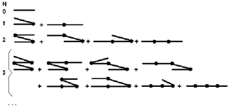
Figure 7: The diagrams that are included in the 1dis-process. The mirror images must also be included, but are not shown

Figure 8: $P_{1dis}$ at $\lambda T=$1, 3, and 5. The ballistic peaks have been artificially broadened for plotting.

While there are $2^{N}$ diagrams at each order, only (N+1) are distinct. Other than the ballistic term, present at every order, we label the remaining $N$ by the index $j$ below. Explicit computation of the this sub-collection yields:

$$\!\!\!\!\!\!\!\!\!\!\!P^{1dis}_{N}(X,T)=\frac{T^{N}}{2^{N}N!}\delta(cT\!-\!X)\!+\!\frac{B(X,cT)N!}{(4c)^{N}}\sum_{j\,=0}^{N-1}\frac{(cT\!+\!X)^{j}(cT\!-\!X)^{N-j-1}}{(n-j)j!^{2}(N-j-1)!^{2}}\;$$ (55)

$B(X,cT)$ is the “Box-car” function defined previously, which maintains the light-cone. We can now insert this result in the summation formula of Eq.(14), and add the parity conjugates, resulting in:

$$\!\!\!\!\!\!\!\!\!\!\!\!\!\!\!\!P^{1dis}(X,T)=\frac{1}{2}\{e^{-\lambda T/2}\delta(cT-X)$$ (56)

$$\;\;\;\;\;\;+\;\;e^{-\lambda T}B(X,cT)\sum_{N=0}^{\infty}\left(\frac{\lambda}{4c}\right)^{N+1}\frac{(cT-X)^{N}}{N!}F\left([-N-1,-N],[1],\rho\right)\}$$

$$\;\;\;\;\;\;+\;\;\frac{1}{2}\{\!X\!\rightarrow\!-X\}.$$

Here $\rho\equiv\frac{cT+X}{cT-X}$, and $F([\alpha,\beta],[\gamma],\rho)$ is the hypergeometric function of the continuous variable $\rho$. Sample behavior of this probability density function is shown in figure-8.

If accuracy is not detrimental, the following simpler expression for the partial probabilities has the same second moment, and approximates the fourth moment of $P^{1dis}_{N}(X,T)$ to within $5\%$,

$$P^{1dis}_{N}(X,T)\simeq\frac{4}{\sqrt{\pi}}\frac{\Gamma\!(\frac{N}{4}\!+\!\frac{3}{2})}{\Gamma(\frac{N}{4})}\frac{T^{N-1}}{N!(N\!+\!2)}\left(1-\frac{X^{2}}{T^{2}}\right)^{N/4-1}$$ (57)

applicable for $N\geq 1$. For $T\leq 5$, the full solution (Eq.(56)) without the ballistic term and the light cone, may also be closely approximated (in units $\lambda=1$, and $c=1$ ) with the form: $const/T^{2}\cdot\exp\{(T\!+3)(1-\!X^{2}/(T\!+3)^{2})^{1/4}\}$, where $const\sim.0022$. The approximation can be very good if one is interested only in small variations in $T$. There, the appropriate value of the const can be found by mere eyeball fitting. For larger T, a gaussian starts to become viable.

7.2 Two-dimensional Isotropic Scattering

In two dimensions, the characteristic function is found by inserting Eq.(53) into Eq.(50):

$$\Phi^{2dis}_{N}(k,T)=\prod_{j\,=0}^{N}\int_{0}^{t_{j\,+1}}\!\!J(0,kc(t_{j\,+1}-t_{j}))\;dt_{j}$$ (58)

where $J(0,x)$ is the zeroth order Bessel function of the first kind. The fourier inversion is made possible via Eq.(29) with the kernel $kJ(0,kR)/2\pi$. For the source emitter configuration, explicit computation yields:

$$P_{N}^{2dis}(R,T)=\frac{\Theta(cT-R)}{2\pi c^{N}(N-1)!}\left(c^{2}T^{2}-R^{2}\right)^{(N-2)/2}$$ (59)

applicable for $N\geq 1$. Summation of orders via the summation rule Eq.(14) yields the full probability density.

$$\!P^{2dis}(X,T)=\frac{e^{-\lambda T}}{2\pi R}\delta(cT-R)+\frac{e^{-\lambda T}\lambda}{2\pi c}\frac{\Theta(cT-R)}{\left(c^{2}T^{2}-R^{2}\right)^{1/2}}e^{\frac{\lambda}{c}\sqrt{c^{2}T^{2}-R^{2}}}.$$ (60)

Note here, that the diffusion limit is found when $cT\!\gg\!R$ rather than the usually assumed limit of $\lambda T\!\gg\!1$. The former, however, is in line with the implications of the central limit theorem, whereas the latter is more of a “rule of thumb”, which must be used with some care. The above two-dimensional results agree with those given in Paasschens .

7.3 Three-dimensional Isotropic Scattering

The 3-dimensional process is likely of greatest practical interest. Below we specialize to the case of the source emitter. Using Eq.(51) we find $Re(\phi_{3})=sin(s_{j})/s_{j}$. Inserting this in Eq.(50) and then into Eq.(29) results in:

$$\!P_{N}^{3dis}(R,T)=\frac{1}{2\pi^{2}Rc}\prod_{j\,=0}^{N}\!\int_{0}^{t_{j\,+1}}\frac{dt_{j}}{\tau_{j}}\int_{0}^{\infty}\!\frac{sin(kR)sin(ck\tau_{j})}{(ck)^{N}}\;dk$$ (61)

where $\tau_{j}\!\equiv\!(t_{j\,+1}\!-\!t_{j})$. As expected, the zeroth order integral produces the ballistic peak: $P_{0}^{3dis}\propto\delta(cT\pm R)$. The first order integrals can be found by convolution of $\phi_{3}$ with $P_{0}^{3dis}$ or, by direct integration to give:

$$P_{1}^{3dis}=\frac{\Theta(cT-R)}{4\pi c^{2}RT}\,\ln\!\!\left(\frac{cT+R}{cT-R}\right).$$ (62)

The result of the sine-transform in Eq.(61), proves inaccessible for $N\!>\!1$. However, the moments of the distribution are easily calculated to arbitrary order. While all odd moments are zero, the even moments are found by the application of $(\nabla_{k}^{2})^{m/2}$ to $\Phi_{N}^{3dis}$, for $m=0,2,4,...$. For $m=0$ normalization can be verified as $M_{N}^{3dis}(0)=T^{N}/(4\pi N!)$. For $m\geq 2$ The $m^{th}$ moment is:

$$M_{N}^{3dis}(m)=\frac{T^{(N+m)}}{4\,\pi^{2}c^{m}}\frac{2^{m/2}\;(N+1)}{(N+m)!\;(m-1)!!}\!\sum_{j\,=0}^{m/2-1}\!\!a_{j}(m)N^{j}$$ (63)

where $(m-1)!!\!=\!\!2^{m/2}\Gamma(\frac{m+1}{2})/\sqrt{\pi}$ for even-$m$ (e.g. $5!!=5\cdot 3\cdot 1$). Only the set $a_{0}(m)=m!^{2}/(2^{m}(m/2)!)$ yields to analytic description. The coefficients $a_{j}(m)$ for up to the eighth moment are listed in the table below.

$a_{j}(m)$	j=0	j=1	j=2	j=3
m=2	1
m=4	18	5
m=6	1350	1715/3	175/3
m=8	264600	137018	22785	1225

For $N\!>\!1$, PaasschensPaasschens has proposed the expression:

$$P_{N}^{3dis}(R,T)\!\simeq\frac{\Theta(cT\!-\!R)}{\pi^{3/2}c^{3}}\frac{\Gamma(\frac{3N}{4}\!+\frac{1}{2})}{\Gamma(\frac{3N}{4})}\frac{T^{N-3}}{N!}\!\left(\!1\!-\!\frac{R^{2}}{c^{2}T^{2}}\!\right)^{\!\!\!\!\frac{3N}{4}-\!1}$$ (64)

for the probability density of the 3dis-process. This expression produces the required second moment exactly, the fourth to within 0.5%, and the sixth moment is approximated to within 1.5%. Hence an excellent approximation for many practical purposes. The total probability density function (via Eq.(14)) has also been approximated by Paasschens :

$$\!\!\!\!\!\!\!\!\!P^{3dis}(R)\simeq\frac{e^{-\lambda T}}{4\pi R^{2}}\delta(cT-R)$$ (65)

$$\;\;\;\;\;\;\;+\;\;e^{-\lambda T}\Theta(cT-R)\frac{(1-R^{2}/c^{2}T^{2})^{1/8}}{(4\pi c^{2}T/3\lambda)^{3/2}}e^{\rho_{3d}}\sqrt{1+2.026/\rho_{3d}}$$

where, $\rho_{3d}\equiv\lambda T(1-R^{2}/c^{2}T^{2})^{3/4}$.

8 Sample Applications

The transmission of photons in turbid media is of interest in medical imaging. During the 1990’s increasingly more successful attempts have been made to model the stochastic movement of the photons in turbid media Durian ; Hindus ; Perelman95 ; Poli ; Miller ; Kaltenbach . Some of these have involved forms of path-integration methods while others, not. However, all of these reports have been limited by varying forms of approximation, limited dimensionality, and the like. Some of these approximations pertain to truncated orders of computation or other more subtle ones such as maintaining the photons’ light-conePerelman95 only on average. Nevertheless, for practical purposes, computations of highly forward-scattering seem suitable for applications involving biological tissues. As such, the findings are in reasonably good agreement within the precision of measurements as reported in Perelman95 ; Winn-Perel98 .

The characteristics of these works have been recounted in a chronological narrative in Hindus . For the case of isotropic scattering, graphical comparisons of several of these works to certain exact results can be found in fig-3.3 of Paasschens .

Here we will not consider the mathematically intricate anisotropic scattering application as it does not make a good illustrative case. The large body of literature in that realm, nevertheless, is good evidence of the struggles of usual approximations with early times ($\lambda T<10$) in stochastic motion. We will however, consider two simpler popular applications of our results: polymer chains, and stock option valuation.

8.1 Flexible Polymer Chains

A minimal model of a flexible polymer is a chain of links of constant length $L$ and total length $x$. By “flexible” we mean that each bond is free to assume any orientation in space as long as it remains linked to its two neighbors. Therefore the probability density distribution of such a chain is a special case of what we have already considered in the Ddis-process where $c(t_{i+1}-t_{i})\!=\!L\!=\!cT/(n+1)$, such that n, the order of computation, is the number of joints. This also means that the often-difficult time-ordered integration becomes unnecessary. That is, back in Eq.(2) the probability of an event at $t_{j}$ is not uniform over $T$ but restricted to the single instant $t_{j}=T/j$. Thus we must use $\delta(t_{j}-\frac{jT}{n+1})dt_{j}$ in place of $\frac{dt_{j}}{T}$, leading to the removal of the time integration in expressions such as Eq.(50) for fixed-sized steps, and resulting in factors which only affect the normalization. Moreover, because of the discovery of the recursion rule in Eq.(51) we need only work out the characteristic function for only one and two dimensions. All higher dimensions can then be derived from these, using the recursion relation.

The one-dimensional case is likely of limited interest but we provide the results here for reference. Using Eq.(52) and Eq.(50)(without the time integration), the characteristic function for a chain of $\ell$ links is the $\ell^{th}$ power of $cos(kL)$, and the effective fourier kernel is $cos(kx)$ for $k\!\in\!(-\infty,\infty)$ and, $x\!\in\!(-\infty,\infty)$. Writing the cosine as exponentials, the transform is easily found as a collection of $\delta$-functions weighted by binomial coefficients:

$$\!\!\!\!\!\!\!P^{1df\!c}_{\ell}(x)=$$

$$\frac{1}{2^{\ell}}\sum_{j=1}^{\frac{\ell+1}{2}}\left({}^{\;\;\;\;\;\ell}_{\frac{\ell+1}{2}-j}\right)(\delta(x\!-\!L(2j\!-\!1))+\delta(x\!+\!L(2j\!-\!1)));\;\;\;\;\ell=1,3,...$$

$$\frac{1}{2^{\ell}}\!\left({}^{\;\,\ell}_{\ell/2}\right)\!\delta(x)+\frac{1}{2^{\ell}}\!\!\sum_{j=1}^{\frac{\ell}{2}}\!\!\left({}^{\;\;\,\ell}_{\frac{\ell}{2}-j}\right)(\delta(x\!-\!2jL)+\delta(x\!+\!2jL));\;\;\;\ell=2,4,...\;\;.$$

It should be apparent that for large $\ell$ the binomial coefficients will tend toward a Normal distribution enveloping the discrete spikes (Fig-9). In that limit, the spikes become indistinguishable and one can approximate $P^{1df\!c}_{\ell}(x=mL)$ as a single term given by $e^{-m^{2}/2n}/\sqrt{2\pi n}$Pearson .

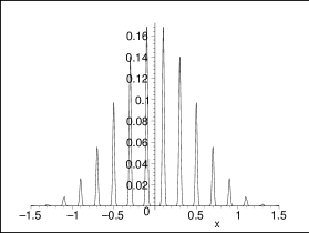
Figure 9: The probability density distribution of Eq.(8.1)) for $\ell=21$ links and $L=0.1$. The peaks have been artificially broadened out for plotting.

The two-dimensional problem has a famous historyPearson but it is easily addressed using our recursion relation. In two-dimensions, using Eq.(53 and 50) the characteristic function for a chain of $\ell$ links is the $\ell^{th}$ power of $J(0,kL)$, and the effective fourier kernel is $kJ(0,kr)$ for both $k$ and, $r\!\in\![0,\infty)$. Despite the fact that the same transformation in conjunction with the time-ordered integration could be worked out in the case of 2dis process, we cannot analytically obtain the probability density function for the end-to-end distance for higher than second order ($\ell\!>\!3$). The zeroth order contains only a single link and obviously corresponds to $\delta(L\!-\!r)/2\pi r$, and the first order is found to be, $\Theta(2L\!-\!r)/\pi^{2}r\sqrt{4L^{2}\!-\!r^{2}}$. The second order (3-link) chain has the probability density for the end-to-end distance, $\textsc{K}(A/\sqrt{L^{3}r})/\pi^{2}\sqrt{L^{3}r}$, for $r\!\in\![L,3L]$, and, $\textsc{K}(\sqrt{L^{3}r}/A)/\pi^{2}A$, for $r\!\in\![0,L]$. Here, K is the complete elliptic integral of the first kind, and $A\!=\!(L+r)\sqrt{L+r)(3L-r)}/4$ is the same as the area subtended by the quadrilateral formed by the the links in the chain and the end-to-end vector of length $r$. As alluded, higher order distributions remain analytically inaccessible. But since we have the exact characteristic function, computing the exact moments at any order is straightforward. Below we provide up to the eight moment, for chains of up to five links.

$M/L^{m}$	m=2	m=4	m=6	m=8
n=0	1	1	1	1
n=1	2	6	20	70
n=2	3	15	93	639
n=3	4	28	256	2716
n=4	5	45	545	7885

For large-$\ell(\simeq n)$, the distribution has been found by a number of methods over the last centuryPearson to approach: $2r/(L^{2}n)e^{-r^{2}/L^{2}n}$.

The most useful case clearly being that of 3-dimension has been worked out by Kleinertkleinert . We find agreement with this result as follows. Specializing Eq.(61) to the problem at hand, we find the characteristic function for a chain of $\ell$ links is the $\ell^{th}$ power of $sin(kL)/kL$, and the effective fourier kernel is $ksin(kr)/2\pi^{2}r$ for both $k$ and, $r\!\in\![0,\infty)$. Because the characteristic function is even in $k$ we can convert the kernel to an exponential and then extend the lower limit to $-\infty$. If we write $sin^{\ell}(kL)$ as combination of exponentials we find an integrand of form $e^{ikx}/k^{\ell-1}$. The full integral can then performed using contour integration resulting inkleinert :

$$P^{3df\!c}_{\ell}(r)=\frac{1}{2^{\ell+1}(\ell-2)!\pi L^{2}r}\sum_{i=0}^{\ell/2}(-1)^{i}\left({}_{i}^{\ell}\right)\left(\ell\!-\!2i\!-\!\frac{r}{L}\right)^{\ell-2}\Theta(L(\ell\!-\!2i)\!-\!r).$$

Here the large-$\ell(\simeq n)$ limit can be shown to be: $\frac{12r^{2}}{nL^{3}}\sqrt{\frac{3}{\pi n}}e^{-3r^{2}/2L^{2}n}$.

8.2 Financial Options Valuation

The problems considered here are especially relevant to the price movements of financial assets. Economists traditionally assume that the logarithm of prices have a normal distributionHull , yet it has always been known this is only true for very large $\lambda$. While this assumption is fine for the intended typical gaseous medium where $\lambda\!\sim\!10^{20}/sec$, the equivalent reset rate for a liquid market is of order inverse daysNYSECharTime . Figure-10, showing the observation-time dependence of the kurtosis over 32 years of S&P log-returns, clearly indicates a finite $\lambda$ and hence the inappropriateness of the diffusion approximation.

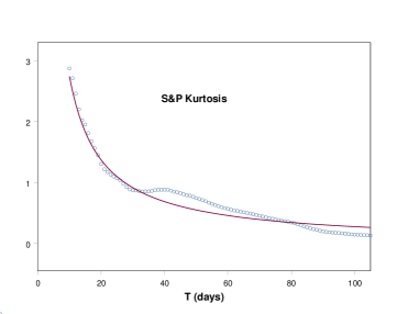
Figure 10: Comparison of the kurtosis for the daily (Jan-1970 to March-2002) log-returns of the S&P500 index vs. a fit of our typical $\kappa\simeq 2/\lambda T$. For $1/\lambda=13.7days$ the agreement is good for periods less than 30 days.

The fact that one cannot fit a single $\lambda$ for different observation-intervals ($T$) (ranging from minutes to many weeks), suggests that more than one process govern different time scalesnotLevy , a notion so common, it is taken for granted by traders. With more than one $P_{gr}$ curve one can arguably reproduce the necessary fat-tails as well as Levy-distributions (figure-11), if only as another alternative.

In order to see some of the implications of finite $\lambda$, we present briefly, the valuation of “options” under the gr-process. Option pricing using path-integrals is quite commonplace; seeLinetsky ; Rosa1 ; Rosa2 ; KleinertOpts to mention only a very few. The computation of the worth of an (European-type) call-option for a non-dividend paying underlying asset was first computed by Black and Scholes BS . A call-option is a contractual right purchased for an agreed upon premium $C$, which gives the buyer a right to purchase a fixed amount of some asset at a later time $T$ from the seller at an agreed upon (“strike”) price $S$. This is regardless of what the prevailing market value of the asset might be at $T$.

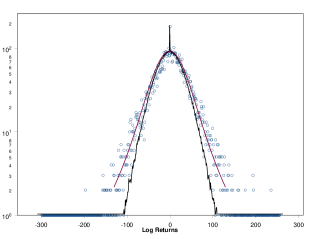
Figure 11: The distribution of log-returns daily (Jan-1970 to March-2002) S&P500 index vs. $P_{gr}$, and Levy distributions. While the Levy curve fits the fat tails much better, a superposition of $P_{gr}$’s can also fit the fat-tails. Conversely, the Levy-distribution does not have the ballistic peak; a feature extant in observation though conveniently ignored by many investigators. Clearly, the correct physical model which gives rise to the Levy-distribution would produce the ballistic peakZumofen . The correct relative amplitude of the ballistic peak to the smooth curve in $P_{gr}$ has not been force-fit.

Black and Scholes(BS) first assumed that the logarithms of the asset’s price follow pure diffusion, with an undetermined diffusion coefficient $\sigma^{2}$ (a.k.a., volatility).The distribution $\delta(lnP-lnP_{0})$ reflects the full certainty that the current price is $P_{0}$. Thus the distribution will spread out in time into a Gaussian of variance $\sigma^{2}T$. They also assumed the log-price to drift linearly (but no faster) in time with an undetermined rate $\mu$ (figure-12). In this way they thought they could fix the price probability density projected for the time $T$ into the future.

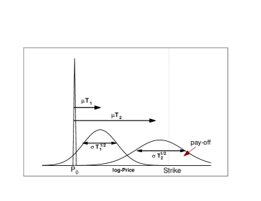
Figure 12: The progression of price distribution according to Black and Scholes

The payoff of an option for the buyer would come about if $P_{T}$ (the market price at time $T$), is higher than the agreed strike $S$; the option expires worthless otherwise. If $P_{T}>S$, the buyer could exercise the said right and immediately sell the asset on the open market for a profit of $P_{T}-S$. Thus a fair price to ask of the buyer is the weighted average of all possible payoffs:

$$C_{BS}=\frac{e^{-rT}}{\sqrt{2\pi\sigma^{2}T}}\int_{\ln S}^{\infty}\!\!dx\,\,(e^{x}-S)e^{-\frac{(x-\ln{P_{0}-\mu T})^{2}}{2\sigma^{2}T}}$$ (68)

where $r$ is the prevailing interest rate. The reason for the pre-factor $e^{-rT}$ is that the buyer loses money by missing out on a steady interest payment since s/he has given up the cash to buy the call-option. BS then argued: if it is true that no-one can win consistently at speculating, the drift rate $\mu$ must exactly be equalr-sigmaSq to the guaranteed interest rate $r$. In this way one of the two arbitrarily introduced parameters was eliminated. The integral can be written with limits $x\!\!\in\![-\infty,\infty]$, if we write the integrand with a step-function. Eq.(68) can then be integrated by parts resulting in an $Er\!f\!c$ (called $N$ in finance texts). The final expression is known as the Black-Scholes formula.

Ostensibly, there are assumptions in the BS hypothesis which are not supported by observation. Conversely, there are many observations which are not incorporated in the BS model, such as Levy-like fat tails in the probability distributionPhysicaA_v269 ; mantegna ; power3 . The resulting discrepancies have become deep puzzles in the realm of financeFinPhil . One such puzzle manifested in the pricing of options is the phenomenon of “price-skew”. In options trading practice the price of an option cannot really be calculated using the BS formula, even after eliminating $\mu$, since the “volatility” ($\sigma^{2}$) is not known. This parameter may be inferred from the variance of the detrended price series of the underlying but using it does not give option prices that match the observation. Conversely, if the observed option values are inserted into the BS formula, the implied volatility $\sigma^{2}$ , resulting from solving:

$$C_{obs}=C_{BS}(S,T,P_{0},r;\sigma),$$ (69)

is not the same as that inferred from observation. In fact, using the observations from different option series (expirations $T$ or strike prices $S$) one gets different values for $\sigma$, whereas $C_{BS}$ only allows a unique value for all options. Ostensibly, there are many more variables which affect $C_{obs}$ in the real world. The existence of any additional variables or control parameters immediately implies that for any given $C_{obs}$, the solution for $\sigma$ is no longer unique. If we take the gr-process as the microscopic basis for the oft-presumed continuous price diffusion (Wiener) process, it provides just such a parameter in the form of $\lambda$.

It will be illustrative to compute the option skew implied by the gr-process. We will do so only in an approximate way so that we need not compute the full $P_{gr}$. This will also clearly demonstrate that the “fat-tail” of the distribution resulting from finite values of $\lambda$ is directly linked to the option-skew phenomenon. We will emulate $P_{gr}$ by matching its kurtosis to that of a superposition of two gaussians (gausslets):

$$G_{2}(x;\nu_{1},\nu_{2})=\frac{e^{-\frac{x^{2}}{2\nu_{1}}}}{2\sqrt{2\pi\nu_{1}}}+\frac{e^{-\frac{x^{2}}{2\nu_{2}}}}{2\sqrt{2\pi\nu_{2}}}.$$ (70)

We can now solve for $\{\nu_{1},\nu_{2}\}$ by setting equal the variance and the fourth moment of $G_{2}$ to that of $P_{gr}$. For illustration sake we can take the intermediate time ($\lambda T>10$) limit of $\nu_{gr}$ Eq. (40), and $\chi_{gr}$ Eq. (41). In this approximation the solutions are:

$$\nu_{1,2}=\frac{s^{2}}{\lambda^{2}}\left(2\lambda T-4\mp 2\sqrt{(2\lambda T-8)}\right).$$ (71)

We can see that if we attempt (as traders do in relying on the BS-model) to fit a single gaussian to the observation, we are likely to be accepting only one of the above variances. It is manifest that the implied volatility has a dependence on the time to expiration $T$ other than the traditional linear term. To demonstrate the same for the strike price $S$ we use the full form of $\nu_{gr}$ and $\chi_{gr}$ and solve for the implied gausslet variances $\{\nu_{1},\nu_{2}\}$. This refined procedure allows us to get to times as low as $\lambda T\simeq 2$, but to go further we must match more moments. We produce an option valuation formula as the half the sum of two Black-Scholes type expressions but using $\{\nu_{1},\nu_{2}\}$ as the respective variances. Settings this approximation to $C_{BS}$ and solving for $\sigma$ for different strikes gives us the the skew curve as shown in the figure-13.

Figure 13: The implied volatility (ordinate) vs. Strike price (abscissa). The two-gausslet ($G_{2}$) representation of $P_{gr}$ is used in place of $C_{obs}$ in Eq(69). Parameter settings are: $\lambda T=10,P_{0}=50,s=0.1,\mu=0,r=0.05$. While the features of skew plot remain the same, their location and span vary to a large extent for different parameters. For this reason one could get a smile, frown, or smirk relative to the at-the-money point $S=P_{0}$. The easiest way to obtain a smirk or a frown is to allow $\mu\neq 0$, this is consistent with the findings in Bouchaud .

The application of the method of path-integrals to financial derivatives’ valuations is a very natural approach. Unlike the case of European (path-independent) options treated above, many options have values which are path-dependent. Hence the valuation must take place as part of the path-integration itself Linetsky ; Rosa1 ; Rosa2 .

9 Acknowledgements

The author gratefully acknowledges M.J.G.Veltman for inspiration for this work on more levels than methodology; K.Osband for encouraging the investigation of problems in finance; and I.M.B.Offen for support and encouragement to complete the work.

Appendix A Damped Exponential Integrals

If it should happen that the gs(d)-process is terminated after a fixed number of events $n$, then the distribution (for the truncated-gaussian-scattering with diffusion) is given by a set of integral functions:

$$\!\!\!\!\!\!\!\!\!P^{tgsd}(x,T)=Dei_{n}(x,T;\lambda,s,\sigma)$$ (72)

$$\;\;\;\;\;\;\;\;\;\;\;\equiv\frac{1}{N^{Dei}_{n}}\int_{0}^{T}e^{-\lambda t_{n}}dt_{n}\int_{0}^{t_{n}}dt_{n-1}\ldots\int_{0}^{t_{2}}dt_{1}\;\;\frac{1}{\xi^{gsd}_{n}}\exp{\!\!\left(-\frac{x^{2}}{2{\xi^{gsd}_{n}}^{2}}\right)}$$

where $Dei$ represents the name “Damped Exponential Integral”. The “interim variance” is defined as before in Eq.(21). The normalization factor is given by:

$$N^{Dei}_{n}=\frac{\sqrt{2\pi}}{\lambda^{n}}\left[1-e^{-\lambda T}\left(\sum_{k=0}^{n-1}\frac{(\lambda T)^{k}}{k!}\right)\right].$$ (73)

Thus $Dei_{0}$ is the familiar normalized Gaussian of width $\sqrt{\sigma^{2}T}$. Further for example, $Dei_{1}$ is a superposition of Gaussians of all variances from $\sigma^{2}T$ to $(\sigma^{2}+s^{2})T$:

$$\!\!\!\!\!\!\!\!\!Dei_{1}(x,T;\lambda,s,\sigma)=\frac{\lambda}{\sqrt{2\pi(1-e^{-\lambda T})}}\int_{0}^{T}dt$$ (74)

$$\;\;\;\;\;\;\;\;\;\;\;\;\;\;\times\;\;\frac{e^{-\lambda t}}{\sqrt{(s^{2}(T-t)^{2}+\sigma^{2}T)}}\;\exp{\left(-\frac{1}{2}\frac{x^{2}}{s^{2}(T-t)^{2}+\sigma^{2}T}\right)}.$$

References

- (1) S. Chandrasekhara, Rev. Mod. Phys. 15, 1 (1943).
- (2) H.Kleinert, Path Integrals in Quantum and Polymer Physics, 3rd ed. (World Scientific, New York 2003), chap.15.
- (3) M.F.M. Osborne, Operations Research. VII, 145 (1959)
- (4) Physica A 269 (1999). The entire volume is dedicated to interesting outstading problems in Econophysics.
- (5) B. Chance, R. R.Alfano, and A. Katzir, eds., Optical Tomography, Photon Migration, and Spectroscopy of Tissue and Model Media: Theory, Human Studies, and Instrumentation, Proc. SPIE 2389 (1995).
- (6) S.Chandrasekhar, Radiative transfer theory (Dover, New York, 1960).
- (7) I.Ishimaru, Wave propagation in Random Media, Vols.1 and 2 (Academic, New York, 1978).
- (8) R.H.J. Kop, P. de Vries,R. Sprik and A. Lagendijk, Phys. Rev. Lett. 79, 4369 (1997).
- (9) S.B.Colak, D.G.Papanicoannou, G.W. ’tHooft, M.B. van der Mark , H.Schomberg, J.C.J.Paaschens, J.B.M.Melissen and N.A.A.J. van Asten, Appl. Opt. 36, 180 (1997).
- (10) L. Wang, P. Ho, C. Liu, G. Zhang and R.R. Alfano, Science, 253, 769 (1991).
- (11) K.M. Yoo, F. Liu and R.R. Alfano, Phys. Rev. Lett., 64, 2647, (1990).
- (12) S. Goldstein, Quarterly J. Mechanics & Appl. Math. & Math. IV, 129(1951). Another author has obtained the same result without apparent knowledge of the latter, though reported a decade later: P.C. Hemmer, Physica 27, 79 (1961).
- (13) D. J. Durian and J. Rudnick, J. Opt. Soc.Am. A 14, 235 (1997); and 14, 940 (1997).
- (14) J.C.J. Paasschens, Doctoral Thesis, Philips Research Laboratories, ch.3, (1997) unpublished. Can be found at: www.lorentz.leidenuniv.nl/beenakker/theses/paasschens/ paasschens.pdf.
- (15) J.M. Porra, J. Masoliver and G. Weiss, Phys. Rev. E 55, 7771 (1997)
- (16) S.A. Ramakrishna and N. Kumar, Phys. Rev. E 60, 1381 (1999)
- (17) V. Pareto, Giornale degli Economisti, Roma, January 1895; V.Pareto, Cours d’economie politique, F. Rouge Editeur, Lausanne and Paris, 1896; reprinted in an edition of his complete works (Vol. III) under the title crits sur la courbe de la repartition de la richesse, Librairie Droz, Geneva, 1965.
- (18) A search at Amazon.com for ”Markov Switching” yields no less than 25 titles, for example: C.-J. Kim, and .R. Nelson State-Space Models with Regime Switching (MIT Press, Cambridge, 1999).
- (19) P. Veronesi, Review of Financial Studies , 12, 975, (1999). For several other interesting works on the “regime switching” phenomenon in trading markets’ behavior see: gsbwww.uchicago.edu/fac/pietro.veronesi/research/.
- (20) H. Kleinert, A. Pelster, M.V. Putz, Phys. Rev. E, 65, 066128 (2002); cond-mat/0202378.
- (21) H. Risken, The Fokker-Plank Equation, 2nd ed., ch.3 (Springer-Verlag Berlin 1989). For a more consice presentation see, H.Risken, Proc. Int’l School in Santander, eds. L. Pesquera, and M.Rodriguez (World Scientific Singapore, 1985).
- (22) P.C. Martin, E.D. Siggia, H.A. Rose, Phys. Rev. A, 8, 423, (1973).
- (23) R.P. Feynman and R.A. Hibbs, Quantum Mechanics and Path Integrals, ch. 12 (McGraw-Hill New York 1965).
- (24) Some of the early mathematics of Path-Integration was developed by Wiener in the context of probability theory: N. Wiener, J. Math. Phys. 2, 131 (1923). N.Wiener, Proc. Math. Soc. 22, 454 (1924). N.Wiener Acta Math. 55, 117 (1930). N.Wiener, Generalized Harmonic Analysis, (MIT Press, Cambridge, 1964). Wiener had even used the term ”path-integral” in the 1923 paper. Earlier attempts by P.J.Daniell dating to 1918 are described in M.Kac, Bull. Am. Math. Soc. 72, 52, (1966).
- (25) G.J. Papadopulous, Path-Integrals and Their Applications, eds. G.J.Papadopulous, and J.T. Deversee, (Plenum Press, New York 1978), pp. 1-71.
- (26) L.F. Richardson, Proc. Roy. Soc. London, SerA 110, 709, (1926)
- (27) J.Klafter, M.F.Shlesinger, G.Zumofen, Physics Today, Feb.1996, p.37.
- (28) M.F.Shlesinger, J.Klafter, B.J. West, Phys. Rev. Lett. 58, 1100, (1987).
- (29) F.W.Wiegel, Introduction to Path-Integral Methods in Physics and Polymer Science, (World Scientific, Singapore 1986), ch. 1.
- (30) L.T. Perelman, J.Wu, Y. Wang, I. Itzkan, R.R. Dasari and M.S. Feld, Phys. Rev. E 51, 6134, (1995).
- (31) A.Ya.Polishchuk, M.Zevallos, F.Liu and R.R. Alfano, Phys. Rev., E 53, 5523 (1996).
- (32) S.D. Miller, J. Math. Phys., 39, 5307, (1998).
- (33) J. Kaltenbach and M. Kaschke, in Medical Optical Tomography: Functional Imaging and Monitoring, edited by G. M uller (SPIE,Washington DC, 1993).
- (34) J. N. Winn, L. T. Perelman, K. Chen, J. Wu, R. R. Dasari, and M. S. Feld, Appl. Optics, 37, 8085 (1998)
- (35) K. Pearson, Nature, 72, 294 (1905), and Lord Rayleigh, Phil. Mag. 37, 321 (1919). For a more modern discussion which gives the same characteristic function as we find, see J.E.Kiefer, and G.H.Weiss, pp.11-32, in ”Random Walks and their application in Physical and Biological Sciences”, AIP, New York, (1984).
- (36) J. Hull, Options, Futures and Other Derivatives, 3rd ed, (Prentice Hall, New Jersey 1996), ch. 10.
- (37) L. Kullmann, J.Toyli, J.Lertesz, A.Kanto, and K.Kaski, op.cit.PhysicaA_v269 , p98.
- (38) We hasten to add that none of the processes exposed here encompass several of the important observations about fiancial markets. Most notably the serially correlated absolute values of returns. These features remain as potential future applications of the present method.
- (39) V. Linetsky, Computational Economics 11, 129 (1998).
- (40) M. Rosa-Clot, S. Taddei, Int. J. Theor. Appl. Finance, 2, 381 (1999); cond-mat/9901277.
- (41) M. Rosa-Clot, S. Taddei, cond-mat/9901279.
- (42) H. Kleinert, Physica A, 312, 217, (2002); cond-mat/0202311
- (43) F. Black, and M. Scholes, J. Political Economy, 81, 637 (1973).
- (44) G.Zumofen, and J.Klafter, Phys. Rev. E 47, 851 (1993) have provided numerical solutions to certain random flights which have an exponental distribution of times between events. The resulting position distributions are of Levy type which correctly display the ballistic peak. See also: J.Klafter, G.Zumofen, and M.F.Shlesigner, pp. 197-215 in Levy Flights and Related Topics in Physics, Eds. M.F.Shlesinger, G.Zaslavsky, and U.Frisch, Springer, Berlin (1995).
- (45) The actual relationship is since there is a lower return rate if the asset price is drifting with variance (op.cit.Hull ).
- (46) R.N. Mantegna, and H.E. Stanley, Nature, 383, 587 (1996)
- (47) P.Gopikrishnan, L.A.N. Amaral, Y. Liu, M. Meyer, V. Plerou, B. Rosenow, and H.E. Stanley, in Unresolved Problems of Noise and Fluctuations, eds.: D. Abbot, and L.B. Kish (AIP, New York, 2000), p.233.
- (48) Like other disciplines branching only recently from philosophy, tradiational theories of finance are founded more on gospelized conjectures, than empirical observations. As such, many of these “puzzles” are more semantic illusions, than genuine mysteries.
- (49) J.-P. Bouchaud, M. Potters, Phil. Trans.: Math. Phys. Engin. Sci. 357, 2019 (1999); cond-mat/9808206.