Optical Manipulation of Long-range Interactions at the 3s+3p Asymptote of Na₂

Abstract

We investigate the influence of a laser field, which is near-resonant to the atomic sodium 3²P_1/2 $\rightarrow$ 3²D_3/2 transition, on the last bound levels of the A${}^{1}\Sigma^{+}_{u}$ state in Na₂. In a molecular beam experiment level shifts up to $\approx$ 100 MHz and light induced line broadenings were observed using an optical double resonance excitation scheme. Moreover, the coupling laser can reduce the number of bound levels of the A state by one or more units, which effectively means that in the picture of a collision of a 3²S_1/2 and a 3²P_1/2-atom the scattering phase is altered by more than $\pi$. The observed effects are interpreted as light induced couplings of the A${}^{1}\Sigma^{+}_{u}$ state, which correlates to the 3s_1/2+3p_1/2 asymptote, to the $4^{1}\Sigma^{+}_{g}$ and $2^{1}\Pi_{g}$ states at the 3s_1/2+3d_3/2 asymptote. We performed multi-channel calculations, applying the mapped Fourier grid method, which reproduce our experimentally observed level shifts well.

1 Introduction

Due to the fast progress in cooling and trapping of ultracold atoms and the achievement of Bose-Einstein condensation An95; Da95; Bra95; Fri98; Ro01; Pe01; Weber02, the interest in a detailed knowledge of ultracold collisional properties has increased Ti96. They are often described by the s-wave scattering length $a_{s}$, which is correlated to the scattering wave function at vanishing collisional energy. It has been shown Cru99; Elbs99; Samu2001 that this important physical quantity can be derived from spectroscopy of the vibrational levels and resonances around the atomic asymptote. But the scattering length is difficult to derive purely on theoretical grounds because it does not only depend on the long-range part of the molecular ground state interaction potentials but also on the accumulated phase from the inner part of the potential.

Beside the knowledge of cold collision properties, the possibilities of their manipulation are central points of interest. It has been shown in Na-Na, Rb-Rb, and recently also in Cs-Cs ultracold collisions that the sign of the scattering length can be altered in the vicinity of a magnetic field induced Feshbach resonance by varying the magnetic field strength In98; Cor00. This offers a wide range of experiments on the dynamics in ultracold ensembles and BEC and a further understanding of two and three particle interaction. Unfortunately, magnetic tuning of two particle interaction is not applicable in typical magnetic traps because the trapping field conditions are affected by the field strength needed according to the desired tuning of the collision conditions.

An alternative approach for the manipulation of cold collisions has been developed in Ma98, where DC electric fields are proposed to control diatomic collisions at ultralow temperatures.

A further promising proposal is the use of near resonant light fields to influence the scattering length $a_{s}$ Fed96; bohn97; kok01. This technique offers the possibility to manipulate the two-particle interaction by coherent light fields. First experiments with photoassociation Fat00 show that it is possible to observe the optical analogue to the magnetic field induced Feshbach resonances if a laser with a frequency close to a photoassociation transition is focused into a magneto optical trap. The study of an optically induced Feshbach resonance is important for possible control of condensate dynamics.

In this paper we follow another approach to determine the effect of near resonant laser light on cold atomic collisions. We use the high resolution of Doppler free spectroscopy on a molecular beam to investigate the effect of a laser field that is near resonant to the atomic sodium 3²P${}_{1/2}\rightarrow$3²D_3/2 transition. Thus, this laser induces a coupling of the A${}^{1}\Sigma^{+}_{u}$ state at the 3s_1/2+3p_1/2 asymptote to states at the 3s_1/2+3d_3/2 asymptote ($4^{1}\Sigma^{+}_{g}$, $2^{1}\Pi_{g}$) with their vibrational and continuum manifold. This results in energy shifts of asymptotic rovibrational energy levels with internuclear separations of about 100 Å in all coupled states modeling atomic pairs with low relative kinetic energy. We extract quantitative information on light induced coupling from the induced level shifts. A similar laser controlled manipulation of the asymptotic ground state potential can be used to investigate schemes to modify the ground state s-wave scattering length $a_{s}$. The advantage of the experiment at the 3s_1/2+3p_1/2 asymptote presented below is the simpler detection via direct laser-induced fluorescence, which is not possible in the case of the ground state asymptote.

This article is organized as follows: First, an outline of our experimental setup and the excitation scheme is given (Section 2). In the following Section 3 we focus on the extraction of quantitative data from the observed line profiles. Experimental results are presented in Section 4. A theoretical model that simulates the investigated light induced energy shifts and line broadenings utilizing a coupled-channel calculation including six channels is developed in Section 5 in the framework of the Mapped Fourier Grid Hamiltonian (MFGH) method involving a complex potential Koko99; pell02. In the concluding section we compare the results of the simulation with the experiment and give also prospects for further experiments and extended simulations.

2 Experiment

We briefly review the experimental setup and focus on the changes made in comparison to Tie96 were we studied asymptotic sodium A state levels within our molecular beam experiment. For the investigation of light induced energy shifts below the asymptote of the A state, we start from molecules in a well collimated beam (molecular velocity of $\approx 1000\>$m/s) which are initially in the lowest vibrational levels ($v_{X}=\>$0, 1) of the $X^{1}\Sigma^{+}_{g}$ ground state (see Figure 1). In a first interaction zone (Figure 2) a Franck-Condon pumping step is applied with laser L1 to create population in thermally unpopulated vibrational levels $v_{X}\approx\>$31 of the ground state. For this purpose a dye laser (sulforhodamine b) operating at about 615 nm is used. Its frequency is stabilized on the maximum of fluorescence of the selected molecular transition.

Figure 1: Potential scheme of Na₂. Laser L1 transfers population to a desired vibrational level ($v_{X}=31$), so that the 3s+3p asymptote can be reached via the second laser L2. The oblique arrow indicates that this laser is scanned during the experiment. A coupling of asymptotic A state levels to the 3s+3p asymptote is induced via the coupling laser L3. The fluorescence from the A state is detected with a lock-in detector synchronized to the chopper frequency of laser L3.

Starting from such vibrationally excited ground state levels the A state asymptote is reached with a tunable dye laser L2 at 532 nm operating with coumarin 6. It is applied in a second interaction zone about 0.35 m downstream from the first zone. The fluorescence from the excited levels is monitored by a photomultiplier. An OG 570 color glass filter suppresses the scattered laser light from L2.

For the manipulation of bound levels close to the A state asymptote a third laser L3 is used. It is an extended cavity diode laser in Littrow configuration operating near the atomic sodium ${\rm 3^{2}P_{1/2}\rightarrow 3^{2}D_{3/2}}$ transition at 818 nm. It is overlapped with L2 by a dichroitic beam splitter and focused into the second interaction zone. In that way a coupling of the A${\rm{}^{1}\Sigma^{+}_{u}}$ state to the 4${\rm{}^{1}\Sigma^{+}_{g}}$ and the $2{\rm{}^{1}\Pi_{g}}$ state at the 3s+3d asymptote is created. The waist radius is $\approx 80\mu$m for L2 and about $\approx 100\mu$m for the laser L3. Overlap and diameter of both beams are controlled with a CCD camera. Both laser beams are linearly polarized, and their polarization axes are parallel to the molecular beam.

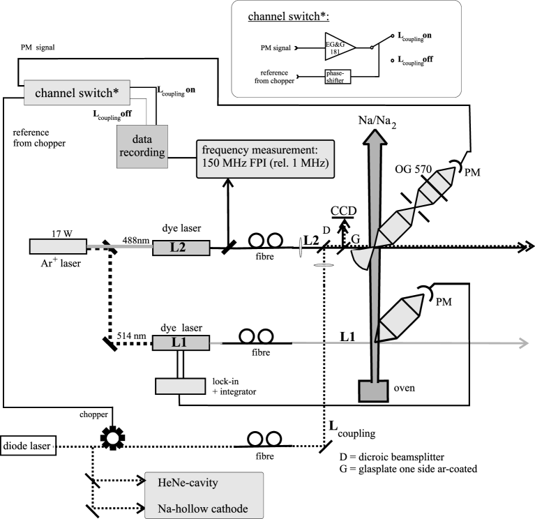
Figure 2: Experimental Setup. A well-collimated molecular beam is crossed by three laser beams. Laser L1 is stabilized on the molecular fluorescence in the first interaction zone, while the fluorescence in the second interaction zone is recorded. The perturbing laser L3 is locked on a stabilized cavity. The signal from the second interaction zone is processed with a channel switch to record a manipulated (L3 on) and unmanipulated (L3 off) spectrum, simultaneously.

For the determination of the atomic transition frequency ${\rm 3^{2}P_{1/2}\rightarrow 3^{2}D_{3/2}}$ we apply optogalvanic spectroscopy in a conventional sodium hollow cathode lamp as reference. By this means a Doppler broadened spectrum of the atomic transition can be obtained. The position of the peak can be determined with an uncertainty of about 30 MHz. For a good long-term frequency stability of L3 it is stabilized to a 150 MHz marker cavity that itself is locked to an iodine stabilized HeNe laser PMT00. Long term drifts of L3 less than 1 MHz/h are achieved in this way. The cavity is locked to the HeNe laser using an acousto-optic modulator (AOM) which allows interpolation between the 150 MHz markers. Hence, we are able to determine the relative detuning with an absolute uncertainty in the order of 1 MHz as long as the cavity is locked to the HeNe laser (see Section 4).

The effect of L3 on the energetic position of asymptotic levels in the A state is observed by a switching technique: L3 is modulated with a mechanical chopper at a frequency of about 1 kHz. The current of the photomultiplier in the second interaction zone is amplified with a fast current amplifier and then fed into an electronic switch, triggered by the chopper signal. It divides the signal into two output channels: The first channel is correlated to ‘L3 off’, the second to ‘L3 on’  if the switching phase is adjusted properly.

Figure 3: A spectrum $\approx 2.5\>$GHz below the asymptote of the A state. L1 was stabilized on the R(6)(17-0) transition, and L2 is tuned across the P(6)/R(6) transitions $v_{X}=31\rightarrow v_{A}=178,179$. The dotted line is a signal with the coupling laser switched off, while the solid one corresponds to the situation when the coupling laser is on ($I_{\rm L3}\approx 74\>$W/cm²). The background results from scattered light of L2. The additional offset in the solid spectrum is due to additional scattered light from the coupling laser. This laser is stabilized in frequency with a detuning of 75 MHz to blue with respect to the atomic sodium 3²P${}_{1/2}\rightarrow$ 3²D_3/2 transition. For both vibrational levels the line profiles of the P and R line are asymmetric. Each line has a shoulder on the low frequency (left) side originating from underlying hyperfine structure.

A typical recorded spectrum, tuning laser L2 while keeping L1 and L3 fixed, is shown in Figure 3. Several scans are averaged to improve the signal-to-noise ratio of the recording. For the presented scan the total integration time per data point was 1s. The Franck-Condon pumping laser L1 is usually stabilized to the A-X R(6) (17-0) transition. The population in $v_{A}\>$=17, $J_{A}\>$=7 decays to $J_{X}\>$=6 and 8 preferentially of vibrational levels around $v_{X}\>$=31. Starting from $v_{X}\>$=31, $J_{X}\>$=6, L2 stimulates the transitions P(6) and R(6) to the asymptotic vibrational levels $v_{A}\>$=178 and 179. The spectrum for every $v_{A}$ thus consists always of two angular momentum components $J_{A}=J_{X}\pm 1$ for each $v_{A}$, to which we refer as P line ($J_{A}=J_{X}-1$) and R line ($J_{A}=J_{X}+1$) in the following. The spectrum is shifted to red (lower frequency) by laser L3, the lines are broader and show asymmetry.

3 Extraction of Line Shifts and Line Broadenings

In this section we explain how we extract information on the line shift $\Delta$ between the manipulated and the unmanipulated trace in a spectrum like in Figure 3. We determine the induced light shift by applying a line shape fit. We deal with the two channels — with and without the coupling laser L3 — simultaneously because the two traces can be described by several common line shape parameters and few additional parameters describing the line shift. It is useful to concentrate on simultaneous simulation of P/R doublets because the two lines overlap for large induced line shifts. The line broadening is determined within the same line shape fit.

For the description of the spectrum several hyperfine components underneath each rotational line have to be taken into account: Due to nuclear spin statistics both P and R line for an even $J_{X}$ have contributions from nuclear spins $I=0,2$. For the latter different orientations with respect to $J_{A}$ appear, which results to 1+5 hyperfine components. For the electric dipole transitions $I$ and $M_{I}$ remain unchanged to good approximation. Each contributing hyperfine component is described by a standard profile

$${{{\rm A}\left[{\rm A_{0}},\nu,\nu_{0}\right]}=\frac{\rm A_{0}}{1+\alpha X^{2}+(1-\beta-\alpha)X^{4}+\beta^{6}X^{6}}}$$ (1)

with

$${{X}={\frac{\nu-\nu_{0}}{\mathrm{HWHM}}}}.$$ (2)

The parameters $\alpha$, $\beta$ and HWHM (half width at half maximum) are equal for all lines contributing to the unshifted spectrum. $\alpha$ and $\beta$ are line profile parameters, which depend on the contribution of the Lorentzian ($\alpha=1,\beta=0$) and residual Gaussian shapes to the line shape. They are determined by the collimation ratio of the experimental apparatus (1:1000) and possibly by frequency jitter. For the profile fits presented here, $\alpha$ has been kept fixed at 1 while $\beta$ is variable.

The fit results show that the observed line profiles can be simulated using the scalar and the tensorial nuclear spin-spin interactions. The center frequency $\nu_{0}$ and the amplitude of each line component thus does not only depend on the rotational quantum number $J_{A}$ and the nuclear spin $I$, but also on the total molecular spin $F=J+I$. The total contribution diagonal in $J$ of the hyperfine interaction to the line position is Bro78:

$$\begin{split}E_{\rm HFS}=&\langle\Omega=0JI^{{}^{\prime}}F|H_{\rm HFS}|\Omega=0JIF\rangle\\ =&\frac{\delta}{2}\delta_{II^{{}^{\prime}}}\bigg{[}I(I+1)-2i(i+1)\bigg{]}\\ &+d\hskip 5.0pti(i+1)(2i+1)(-1)^{I^{{}^{\prime}}+F+1}\\ &\times\bigg{[}30(2I+1)(2I^{{}^{\prime}}+1)\bigg{]}^{1/2}\\ &\times(2J+1)\left(\begin{array}[]{ccc}J&J&2\\ 0&0&0\end{array}\right)\left\{\begin{array}[]{ccc}F&I^{{}^{\prime}}&J\\ 2&J&I\end{array}\right\}\left\{\begin{array}[]{ccc}i&i&1\\ i&i&1\\ I&I^{{}^{\prime}}&2\end{array}\right\}.\end{split}$$ (3)

$\vec{I}$=$\vec{I^{{}^{\prime}}}$=$\vec{i}_{1}$+$\vec{i}_{2}$ is the total nuclear spin, $i=i_{1}=i_{2}=3/2$ is the nuclear spin of a single sodium atom and Wigner’s symbols are used. The first term in equation (3) is the scalar part of the hyperfine interaction while the second one is the tensorial contribution of the hyperfine energy. The $\delta$-parameter for the scalar and the $d$-parameter for the tensorial part depend on the states mixed by the hyperfine interaction. At the 3s+3p asymptote a large variety of states is coupled to the A state, so that the functional dependence of the ratio of $\delta$ and $d$ does not have a simple analytic form. Thus, for the P/R line we let both parameters vary in the fit. The quadrupole and magnetic rotation hyperfine interactions are negligible in the present case of asymptotic levels.

For the profile simulations, we assume that all hyperfine components for a single $J$ resulting from equation (3) are of equal intensity and thus we need two parameters for the description of the intensities of each P/R doublet. This assumption would be not sufficiently good for small angular momenta $J,F$. For the positions of P and R lines $\nu_{0}=\nu_{v}+B_{v}J_{A}(J_{A}+1)+E_{\rm HFS}$ is used. For every $v_{A}$ the unperturbed profile is composed by (for even $J_{X}$)

$$U\left(\nu\right) = U_{\rm off}+\sum_{J_{A}=J_{X}\pm 1}\hskip 4.30554pt\sum_{I=0,2}$$

$$\sum_{F=\left|J_{A}-I\right|}^{J_{A}+I}{\rm A}\big{[}{\rm A_{0}}\left(I,F,J_{A}\right),\nu,\nu_{0}\left(I,F,J_{A}\right)\big{]},$$

with $U_{\rm off}$ to account for a background offset in the experimental trace.

For the simulation of the recordings with the coupling light field on, we use the same parameters $\alpha$ and $\beta$ but a different HWHM. It can be larger than without coupling laser due to predissociation broadening induced by the optical coupling to the upper states ($4^{1}\Sigma^{+}_{g}$, $2^{1}\Pi_{g}$, see discussion below).

The offset of the trace recorded with coupling laser $S_{\rm off}$ differs from the offset $U_{\rm off}$ of the uncoupled trace as the detector sees some additional scattered light originating from the coupling laser. We introduce an additional parameter for the description of the absolute intensities of both P and R line of the shifted spectrum.

A coupling laser field causes the splitting of a line at $\nu_{0}$ into two Autler-Townes components at $\nu_{0}\pm\Delta$. The line shift $\Delta$ and the relative weight of the Autler-Townes components of each line depend on the frequency of the coupling laser and on the Rabi frequencies of the coupling transitions. For P and R line the ratio of the intensities of the two Autler-Townes components are fitting parameters and are later called $q_{J_{A}}$. Due to reasons discussed below the shifted doublet is composed of various lines with different shifts $\Delta$.

The geometries of the laser beams L2 an L3 need to be considered for a proper simulation: The detection probability is proportional to the local intensity of L2, $I_{\rm L2}(r)$, and as the dipole coupling is $M$ dependent, the induced shift is a function of $M$ and of the local intensity of L3, $I_{\rm L3}(r)$.

As the polarization vector of L2 and of L3 are defined in the laboratory frame and the transition moments of the molecules are given in the molecular frame a transformation between those two systems has to be performed. We assume that the projection $M$ of the angular momentum $J$ onto to the laser polarization vector remains unchanged in the second interaction zone, and that all $M$ are equally populated. The latter assumption is justified as we start from a thermal molecular beam and the light of L1 is unpolarized.

As P, R, and Q (state $2^{1}\Pi_{g}$) coupling contribute to the induced shift of a level for a specific $M$, the $M$-dependence is not the regular parabolic dependency as for a single P, Q, or R coupling like $M^{2}$ or $J^{2}-M^{2}$ that results from the direction cosine matrices. We derived from a simulation with diabatic, rotationally corrected potentials and ab initio coupling strengths (see Section 5) that for large internuclear distances the shift $\Delta$ resulting from P, Q, and R coupling can be factorized into a function parabolic in $M$ and linear in $I_{\rm L3}$:

$${{\Delta\left(M,I_{3}\right)}\sim{I_{\rm L3}\left[1-b\left(\frac{M}{J_{A}}\right)^{2}\right]}}$$ (5)

We derived $b=0.7$ in our simulation. This result of potential shift calculations at large internuclear distance is applied to asymptotic levels because in such cases the main contribution of the overlap integral of the vibrational wave functions results from large internuclear separations.

For the geometric model of the laser intensity distribution we assume Gaussian TEM₀₀ laser modes. Although the beams L2 and L3 are focused (waist $w_{0}^{2,3}$) into the second interaction zone, we can assume that we have plane waves because the Rayleigh ranges $z_{R}^{2,3}$ are larger than the radius of the detection zone $\rho$ ($w_{0}^{i}\ll\rho\ll z_{R}^{i}$). With good approximation we can assume that the molecular density is constant in the observed zone. Taking the cylindrical symmetry of the laser fields into account, the description of the space dependent interaction can be reduced to one coordinate: the radial distance $r$ from the common axis of the laser beams L2 and L3. We define as an approximation to a Gaussian profile a distribution of a discrete number $p_{\max}$ of equi-thick hollow cylinders. In each of them we assume a constant intensity $I_{\rm L2}^{p}$ and $I_{\rm L3}^{p}$ representing the average intensity of L2 and L3 in the cylinder $p$ where $p$ counts from the center to the outer range.

With this model the profile of one Autler-Townes component of one rotational line $J_{X}\rightarrow J_{A}$ with an unperturbed transition frequency $\nu_{0}$ can be described as follows:

$${\rm T^{\pm}}\left[\nu,\nu_{0},J_{A},{\rm A_{0}}\right]\sim\sum_{M=-J_{X}}^{J_{X}}\left(\begin{array}[]{ccc}J_{A}&1&J_{X}\\ -M&0&M\end{array}\right)^{2}$$ (8)

$$\times\sum_{p=1}^{p_{\max}}\frac{2p-1}{p_{\max}^{2}}\;I_{\rm L2}^{p}\;{\rm A}\big{[}\nu,\nu_{0}\pm\Delta(M,I_{\rm L3}^{p}),{\rm A_{0}}\big{]}.$$

The Wigner 3j-symbol gives the relative detection probability for a single $M$ in the unsaturated case for L2 and $\frac{2p-1}{p_{\max}^{2}}$ is the statistical weight for the hollow cylinder $p$ of molecules. Like for the unshifted spectra described by equation (3), the summation over all contributing lines needs to be performed for the shifted spectra, too:

$$S\left(\nu\right)=S_{\rm off}+\sum\limits_{J_{A}=J_{X}\pm 1}\hskip 4.30554pt\sum\limits_{I=0,2}\hskip 4.30554pt\sum\limits_{F=\left|J_{A}-I\right|}^{J_{A}+I}$$ (9)

$$\times\bigg{[}q_{J_{A}}^{\pm}{\rm T^{+}}\big{[}\nu,\nu_{0}\left(I,F,J_{A}\right),J_{A},{\rm A_{0}}\left(I,F,J_{A}\right)\big{]}+$$

$$\hskip 12.91663pt\left(1-q_{J_{A}}^{\pm}\right){\rm T^{-}}\big{[}\nu,\nu_{0}\left(I,F,J_{A}\right),J_{A},{\rm A_{0}}\left(I,F,J_{A}\right)\big{]}\bigg{]}.$$

The intensity ratios of the Autler-Townes components $q_{J_{A}}^{\pm}$ are limited by $0\leq q_{J_{A}}^{\pm}\leq 1$ and are either almost 0 or almost 1 because the detuning of L3 from the coupling transitions is rather large compared to the Rabi frequency (see above).

In the following the derived parameter of the level shift corresponds to the maximal shift, i.e., the shift for $M=0$ molecules at the beam center, $\Delta(0,I_{\rm L3})$ in equation (5).

Figure 4: Experimental and simulated spectrum of $v_{A}=178$, $J_{A}=5,7$. The dotted trace is the unshifted experimental spectrum. The dashed trace is the shifted experimental one (coupling laser on the atomic 3²P${}_{1/2}\rightarrow~{}3^{2}$D_3/2 resonance, $I_{\rm L3}=\>$74 W/cm²). The two solid traces correspond to the simulation of the spectra as explained in the text.

Figure 4 shows the result of a fit to an experimental spectrum for $v_{A}=178$. The experimental traces are plotted in dotted (unshifted) and dashed style (shifted). L3 was resonant to the 3²P${}_{1/2}\rightarrow$3²D_3/2 transition and caused an intensity of $I_{\rm L3}=74\>$W/cm². The criterion for the quality of the fit is the sum of squared difference between experimental and fitted points. The agreement between experimental and fitted line profiles is within the noise interval. The line shift obtained from the fit is -28.9 MHz for $J_{A}\>$=5 and -29.7 MHz for $J_{A}\>=$7 in the above case. The uncertainty of the shifts can be estimated by varying the starting conditions of the fit and is determined to be less than 3 MHz here.

4 Experimental Results

The dependence of the light induced energy shifts of $v_{A}\>=173,\dots,182,$ $J_{A}\>$=5,7 on power and detuning of the coupling laser L3 has been investigated. First we will focus on the effect on the last bound levels directly below the A state asymptote. Figure 5 shows a spectrum of the levels $v_{A}=181$ to 184. The trace plotted in dotted style is recorded without the coupling laser while the second trace, plotted in solid style, is recorded in presence of the coupling laser field. The intensity of the coupling laser was set to $I_{\rm L3}=43$ ${\rm W/cm^{2}}$ and the frequency was stabilized 75(30) MHz blue detuned with respect to the atomic 3²P${}_{1/2}\rightarrow$3²D_3/2 transition. All levels are shifted to lower frequencies or energies, note the position of the potential asymptote. Additionally, the line profiles of the levels $v_{A}\>=182$ to 184 have remarkably changed: The lines are broader than without the coupling laser. The P and the R line start to overlap. The dissociation continuum has been shifted, $v_{A}=184$ disappears.

Figure 5: Effect of the optical manipulation on the last vibrational levels of the A state. The coupling laser is 75(30) MHz blue detuned with respect the atomic 3²P${}_{1/2}\rightarrow$3²D_3/2 transition. The intensity is 43 W/cm². The dotted spectrum is recorded in absence of the coupling laser while the solid one is recorded with coupling laser switched on.

In Figure 6 the variation of the observed shifts of $v_{A}\>$=178, $J_{A}\>$=5 as a function of the intensity of the coupling laser is shown. The laser frequency of L3 was kept fixed 75(30) MHz blue detuned as before, but the intensity was varied from 15 to 67 W/cm². This corresponds to energy shifts in the central region of the beam up to 26.9(30) MHz. The dependence of the shift on the laser intensity is linear within the experimental accuracy.

The error limits for the absolute intensity result mainly from the uncertainty in the determination of the focus diameter of the coupling laser beam. We use for this purpose a CCD camera with a pixel size of 23$\mu$m $\times$ 27$\mu$m, on which we project a 10% reflex of each laser beam of the second interaction zone. The CCD and the second interaction zone are equi-distant from the beam splitter, so that the beam diameter measured with the CCD is the same as the focus diameter in the second interaction zone and can be derived with an absolute uncertainty of one pixel size of the CCD chip which results in the 50% uncertainty for the determination of the coupling laser intensity. The relative change of the intensity in Figure 5 is known with an uncertainty of 5%, limited by the uncertainty of the power meter.

Figure 6: Dependence of the light shift of $v_{A}\>$=178, $J_{A}\>$=5 on the intensity of the coupling laser. Without coupling laser this level is bound by 2646 MHz. The frequency of the coupling laser is stabilized 75(30) MHz blue detuned from the atomic 3²P${}_{1/2}\rightarrow$3²D_3/2 transition. The absolute uncertainty of the coupling laser intensity is 50% and originates from the resolution of the beam view camera utilized for the determination the laser beam diameters. The relative uncertainty between different measurements is less than 5%.

As an example for the dependence of level shifts on the detuning of the coupling laser experimental shifts of $v_{A}\>$=179, $J_{A}\>$=7 are plotted in Figure 10. The reference frequency for the detuning is the energy difference $\delta\omega$ from $v_{A}\>$=179, $J_{A}\>$=7 to the 3s_1/2+3d_3/2 asymptote. This is reasonable because in the region of the outer turning point of the A state vibrational wave function (where the coupling is induced) the potential of the upper 3s+3d asymptote has almost reached its asymptotic value. This is due to the $1/R^{5}$-dependence from a quadrupole-quadrupole coupling of a s-electron and a d-electron and is in contrast to the $1/R^{3}$-behavior of the resonant dipole-dipole interaction of the A state potential correlated to the s+p asymptote. For the series of measurements in Figure 10 the laser intensity of the coupling laser was held fixed at 74 W/cm². The circles in Figure 10 are results from simulations, which we will describe in the following section.

5 Theoretical Interpretation

The observed level shifts originate from the laser-induced dipole coupling of the A${}^{1}\Sigma^{+}_{u}$ state to the 4${}^{1}\Sigma^{+}_{g}$ and the 2${}^{1}\Pi_{g}$ states, both correlated to the 3s+3d asymptote (Figure 1). We use a dressed molecule picture similar to Vat01 for the simulation of the coupled system. After eliminating the explicit time dependence from the theoretical model, a mapped Fourier grid method Koko99 is used to determine line positions and light induced line broadenings.

For the correct description of the dipole coupling we have to take care of the e/f symmetries of the involved rotational levels and the selection rules for an optically induced dipole coupling. Thus, the A state can only couple to the $4^{1}\Sigma^{+}_{g}$ state on a P and R line, while there is P, Q, and R coupling to the $2^{1}\Pi_{g}$-state. For a proper symmetrization, the latter state usually is expressed as a linear combination $|2^{1}\Pi_{g}\rangle=\frac{1}{\sqrt{2}}\left(|\Omega=1\rangle\pm(-1)^{J}|\Omega=-1\rangle\right)$. The plus sign gives the e component of the $\Pi$-state that can only be reached by P and R couplings, while the minus is the f component which couples to the A state by a Q line. For each $M$ (projection of $J$ onto space fixed axis neglecting hyperfine structure), a coupled system can be calculated. Thus, the system to be solved consists of six (except five for $M$=0, where the Q coupling for $\Sigma\rightarrow\Pi$ vanishes) coupled channels, as illustrated in Figure 7.

Figure 7: Potential scheme of the dipole coupling of A${}^{1}\Sigma^{+}_{u}$ state to the 4${}^{1}\Sigma^{+}_{g}$ and the 2${}^{1}\Pi_{g}$ states. Dipole selection rules allow P and R coupling to the 4${}^{1}\Sigma^{+}_{g}$-state, and P, Q, and R coupling to the 2${}^{1}\Pi_{g}$-state. The inset shows the rotational barriers at the $3s+3d$ asymptote for $J_{A}=7$.

The coupled system is described by a six component wave function. For a simple notation we use $G$, $\Sigma$, and $\Pi$ instead of A${}^{1}\Sigma^{+}_{u}$, 4${}^{1}\Sigma^{+}_{g}$, and 2${}^{1}\Pi_{g}$ for the electronic part of the wave functions. With Born-Oppenheimer basis functions, the coupled channel wave function thus can be expressed as

$$\begin{split}\vec{\Psi}(R,t)=&\left(\begin{array}[]{r}\Psi_{G}^{(J)}(R,\vec{r}_{k},t)\\ \Psi_{\Sigma}^{(J-1)}(R,\vec{r}_{k},t)\\ \Psi_{\Sigma}^{(J+1)}(R,\vec{r}_{k},t)\\ \Psi_{\Pi}^{(J-1)}(R,\vec{r}_{k},t)\\ \Psi_{\Pi}^{(J)}(R,\vec{r}_{k},t)\\ \Psi_{\Pi}^{(J+1)}(R,\vec{r}_{k},t)\\ \end{array}\right)\\ =&\left(\begin{array}[]{rcl}\frac{1}{R}\chi_{G}(R,t)&\phi_{G}(\vec{r}_{k};R)&|\xi_{J}\rangle\\ \frac{1}{R}\chi_{\Sigma}(R,t)&\phi_{\Sigma}(\vec{r}_{k};R)&|\xi_{J-1}\rangle\\ \frac{1}{R}\chi_{\Sigma}(R,t)&\phi_{\Sigma}(\vec{r}_{k};R)&|\xi_{J+1}\rangle\\ \frac{1}{R}\chi_{\Pi}(R,t)&\phi_{\Pi}(\vec{r}_{k};R)&|\xi_{J-1}\rangle\\ \frac{1}{R}\chi_{\Pi}(R,t)&\phi_{\Pi}(\vec{r}_{k};R)&|\xi_{J}\rangle\\ \frac{1}{R}\chi_{\Pi}(R,t)&\phi_{\Pi}(\vec{r}_{k};R)&|\xi_{J+1}\rangle\\ \end{array}\right),\end{split}$$ (10)

where $R$ is the distance of the two nuclei and $\vec{r}_{k}$ are the coordinates of the electrons in the molecular frame. $|\xi_{J}\rangle$ are the basis functions for the rotation for an angular momentum $J$. $\phi_{G}(\vec{r}_{i};R)$, $\phi_{\Sigma}(\vec{r}_{i};R)$, and $\phi_{\Pi}(\vec{r}_{i};R)$ are the electronic wave functions corresponding to the potential curves $U_{G}$, $U_{\Sigma}$, and $U_{\Pi}$. The functions $\chi_{G}$, $\chi_{\Sigma}$, and $\chi_{\Pi}$ describe the radial motion in these potentials.

The Hamiltonian of the coupled system divides into two parts:

$$\underline{\hat{\bf H}}=\underline{\hat{\bf H}}^{\rm mol}+\underline{\hat{\bf W}}.$$ (11)

The molecular part of the Hamiltonian $\underline{\hat{\bf H}}^{\rm mol}$describes the field free case, whereas the second part $\underline{\hat{\bf W}}$ describes the dipole coupling between the different electronic states. Both matrices are set up as a matrix of $k\times k$ blocks where $k$ is the number of coupled channels. The diagonal blocks of $\underline{\hat{\bf H}}^{\rm mol}$ are the matrixes $\hat{\bf H}^{\rm mol}_{i}\left(1\leq~{}i\leq~{}k\right)$, all non-diagonal blocks vanish. $\underline{\hat{\bf W}}$ is set up of $\hat{\bf W}_{ij}\left(1\leq~{}i,j\leq~{}k\right)$. $\hat{\bf W}_{ij}$ represents the dipole coupling between the states of channel $i$ and $j$. $\hat{\bf W}_{ij}$ vanishes if $i$ and $j$ are equal or if none of the channels $i,j$ is $G$. Operators denoted with underscore, i.e., $\underline{\rm\hat{\bf H}}$, represent operators that act on all channels (in our case five or six for all internuclear distances). In contrast operators without underscore represent operators that either act on one channel only or describe the coupling of exactly two channels ($\hat{\bf H}^{\rm mol}_{i}$ resp. $\hat{\bf W}_{ij}$).

$$\begin{split}&\hat{\bf H}^{\rm mol}_{i}=\hat{\bf T}_{i}+\hat{\bf U}_{i}\\ &+\frac{\hbar^{2}\left[J\left(J+1\right)+S\left(S+1\right)+L\left(L+1\right)-\Omega^{2}-\Sigma^{2}-\Lambda^{2}\right]_{i}}{2\mu R^{2}}\end{split}$$ (12)

is the molecular part of the Hamiltonian. $\hat{\bf T}_{i}$ is the kinetic energy operator and $\hat{\bf U}_{i}$ the electronic potential energy operator of the electronic state $i$. The third term is the rotational energy of the two nuclei relative to each other represented in Hund’s coupling case (a). $\mu$ is the reduced mass of the molecule.

The coupling laser L3 is assumed to be a plane and monochromatic wave with frequency $\omega_{L}$. Thus, in dipole approximation

$$\hat{\bf W}\left(t\right)_{ij}=-\vec{D}_{i,j}(R)\cdot\vec{\epsilon}_{L}E_{0}\frac{1}{2}\left(e^{i\omega_{L}t}+e^{-i\omega_{L}t}\right).$$ (13)

$\vec{D}_{i,j}(R)$ is the dipole moment for the transition between the electronic states $\phi_{i}$ and $\phi_{j}$ resulting from the integration over $\vec{r}_{k}$ according to equation (10). $\vec{D}_{i,j}(R)$ vanishes for transitions between $\Sigma$- and $\Pi$-state because $g\leftrightarrow g$ couplings are forbidden by electric dipole selection rules. $\vec{\epsilon}_{L}$ describes the unity vector in the direction of the laser polarization and $E_{0}$ is the electric field strength.

With this Hamiltonian, the time-dependent Schrödinger equation for the six-components wave function $\vec{\Psi}(t)$ is:

$$i\hbar\frac{\partial}{\partial t}\vec{\Psi}(R,t)=\left[\underline{\hat{\bf H}}^{\rm mol}+\underline{\hat{\bf W}}(t)\right]\vec{\Psi}(R,t)$$ (14)

Figure 8: Asymptotic region of the coupled electronic potentials. The A state potential is dressed by a photon energy of the coupling laser L3. The energy difference $\Delta\omega$ is due to the detuning of the coupling laser relative to the atomic transition. $\delta\omega$ is the relative position of one individual vibrational level $v_{A}$ to the 3s_1/2+3d_3/2 asymptote within the dressed state picture.

The radial wave functions for the nuclear motion in the electronic channels at the lower and upper asymptote are transformed via

$$\chi_{G}(R,t)=\tilde{\chi}_{G}(R,t)\exp(i\Delta\omega t),$$

$$\chi_{\Sigma}(R,t)=\tilde{\chi}_{\Sigma}(R,t)\exp(-i\omega_{0}t),$$ (15)

$$\chi_{\Pi}(R,t)=\tilde{\chi}_{\Pi}(R,t)\exp(-i\omega_{0}t),$$

where $\omega_{0}$ (see Figure 7) is the transition frequency of the atomic 3²p_1/2 $\rightarrow$ 3²d_3/2-transition, $\Delta\omega$ is the detuning of the coupling laser with respect to $\omega_{0}$ ($\Delta\omega=\omega_{L}-\omega_{0}$). By the transformation (5) we shift (dress) the origin of energy for the electronic potentials,

$$\tilde{U}_{G}(R)=U_{G}(R)+\hbar\Delta\omega,$$

$$\tilde{U}_{\Sigma}(R)=U_{\Sigma}(R)-\hbar\omega_{0},$$ (16)

$$\tilde{U}_{\Pi}(R)=U_{\Pi}(R)-\hbar\omega_{0}.$$

Hence, all three electronic potentials have almost the same asymptotic energies. In Figure 8 the resulting molecular potentials dressed by one photon of a blue detuned (relative to the atomic transition) coupling laser are plotted.

Adapting the dressed potentials in the $\hat{\bf H}^{\rm mol}_{i}$, the Schrödinger equation (14) for the vibrational motion in the six coupled channels can be written as

$$\begin{split}&i\hbar\frac{\partial}{\partial t}\left(\begin{array}[]{r}\tilde{\chi}_{G}^{J}(R,t)\\ \tilde{\chi}_{\Sigma}^{J-1}(R,t)\\ \tilde{\chi}_{\Sigma}^{J+1}(R,t)\\ \tilde{\chi}_{\Pi}^{J-1}(R,t)\\ \tilde{\chi}_{\Pi}^{J}(R,t)\\ \tilde{\chi}_{\Pi}^{J+1}(R,t)\\ \end{array}\right)=\\ &\left(\begin{array}[]{cccccc}{\bf H}^{\rm mol}_{G_{J}}&\hbar{\bf\Omega}_{\Sigma}^{-1}&\hbar{\bf\Omega}_{\Sigma}^{+1}&\hbar{\bf\Omega}_{\Pi}^{-1}&\hbar{\bf\Omega}_{\Pi}^{0}&\hbar{\bf\Omega}_{\Pi}^{+1}\\ \hbar{\bf\Omega}_{\Sigma}^{-1}&{\bf H}^{\rm mol}_{\Sigma_{J-1}}&0&0&0&0\\ \hbar{\bf\Omega}_{\Sigma}^{+1}&0&{\bf H}^{\rm mol}_{\Sigma_{J+1}}&0&0&0\\ \hbar{\bf\Omega}_{\Pi}^{-1}&0&0&{\bf H}^{\rm mol}_{\Pi_{J-1}}&0&0\\ \hbar{\bf\Omega}_{\Pi}^{0}&0&0&0&{\bf H}^{\rm mol}_{\Pi_{J}}&0\\ \hbar{\bf\Omega}_{\Pi}^{+1}&0&0&0&0&{\bf H}^{\rm mol}_{\Pi_{J-1}}\\ \end{array}\right)\left(\begin{array}[]{r}\tilde{\chi}_{G}^{J}(R,t)\\ \tilde{\chi}_{\Sigma}^{J-1}(R,t)\\ \tilde{\chi}_{\Sigma}^{J+1}(R,t)\\ \tilde{\chi}_{\Pi}^{J-1}(R,t)\\ \tilde{\chi}_{\Pi}^{J}(R,t)\\ \tilde{\chi}_{\Pi}^{J+1}(R,t)\\ \end{array}\right),\end{split}$$ (17)

where $J$ is short for $J_{A}$ used in the other sections.

To solve this multi-channel problem the explicit time dependence of the Hamilton operator can be eliminated if the rotating wave approximation Bws90 is applied. It is based on the suppression of the fast oscillating terms in the coupling matrix elements, which average out over times given by the vibrational period of the molecule.

The coupling matrix elements between the $G$ (originally the A state) and electronically higher excited states $\Sigma$ and $\Pi$ are expressed by time independent Rabi frequencies ${\bf\Omega}_{j}^{\beta}(R)/2\pi$ ($j=\Sigma,\Pi$) where $\beta=0,\pm 1$ indicates the difference of the rotational quantum number between the coupled states. They are related to the electronic transition dipole moment by

$$\hbar{\bf\Omega}_{j}^{\beta}(R) = -\;\;\frac{1}{2}\;\;\;E_{0}\;\;\;|\vec{D}_{G,j}(R)|\left(\begin{array}[]{ccc}J\!\!+\!\beta&1&J\\ -M&0&M\end{array}\right)$$ (20)

$$= -\frac{1}{2}\sqrt{\frac{2I_{\rm L3}}{c\epsilon_{0}}}\ |\vec{D}_{G,j}(R)|\left(\begin{array}[]{ccc}J\!\!+\!\beta&1&J\\ -M&0&M\end{array}\right).$$ (23)

Here we take into account the earlier discussed $M$-dependence by the linear polarized light in the experiment. For each projection of $M$ on the laboratory frame the eigenvalue problem of the coupled channel system gives the stationary solution and can be solved for each $M$ separately. Levels with different $M$ do not couple.

The light induced energy shifts (the difference of corresponding eigenvalues with and without light field) and line broadenings are computed using the Mapped Fourier Grid Hamiltonian (MFGH) representation, described in detail in Koko99. The MFGH method has been designed in the context of photoassociation of cold atoms and cold molecule formation, where interactions at large internuclear distances play the key role. In subsequent papers Koko00; pell02, a complex potential has been introduced to treat the interaction of bound levels embedded into dissociation continua. Here we recall only the main steps of the MFGH method:

• In the standard Fourier Grid Hamiltonian (FGH) method, the total Hamiltonian for the coupled channels is expressed in a basis on $N$ plane waves, $\exp\bigg{(}{\frac{i2\pi kR}{L}}\bigg{)}$, $k=-(\frac{N}{2}-1),\dots,0,\dots,\frac{N}{2}$, where $L$ is the range of internuclear distances under investigation. The diagonalization yields eigenfunctions represented as an expansion over the same basis, the coefficients being the value of the wave function at each point of the grid of length $L$ with $N$ equi-distant points.

• As the local de Broglie wavelength of wave functions varies by orders of magnitude between the small and the large internuclear distance range, an adaptative coordinate can be defined in the FGH framework, which maps the variation of the local kinetic energy. The number of required grid points is reduced substantially, allowing accurate calculations of energy levels with large elongations, i.e., close to the dissociation limit.

• The width of the energy levels interacting with a dissociation continuum is obtained after the diagonalization of the total Hamiltonian, including a pure imaginary potential (or an optical potential) $V_{\rm opt}$ placed at large distances, which ensures absorbing boundary conditions for the outgoing waves. In a stationary approach, the dissociating wave functions behave asymptotically as Siegert states pell02. We choose the form proposed in Vib92:

  $$V_{\rm opt}=A_{\rm opt}N_{\rm opt}exp\bigg{(}\frac{-2L_{\rm opt}}{R-R_{\rm opt}}\bigg{)},$$ (24)

  where $N_{\rm opt}$ is a normalization factor, $R_{\rm opt}$, $L_{\rm opt}$ and $A_{\rm opt}$ are respectively the position, the length, and the amplitude of the optical potential. The values of these parameters are chosen according to the recommendation of Vib92. The imaginary part of the eigenvalues resulting from the diagonalization of the Hamiltonian matrix provides the predissociation line width

In our calculations, we used a grid with $L\>$=1100 a.u.(1 a.u. =$0.5291772083\times 10^{-10}$ m), with typically 700 grid points, which induces a diagonalization of 4200$\times$4200 squared matrix, using standard LAPACK routines. As we are looking for very small energy shifts, a high accuracy is needed for the eigenvalues, which is checked by studying their convergence depending on the contraction (equal to 0.2 here) of the grid step. A contraction of 1 corresponds to a local grid density of four points per local de Broglie wavelength. The optical potential is set up to absorb outgoing waves with kinetic energies corresponding to the detuning $\Delta\omega$ of the coupling laser L3, following the rules described in Vib92. The parameter values are $A_{\rm opt}=5.6\times 10^{-7}$ a.u., $L_{\rm opt}=210$ a.u., $R_{\rm opt}=L-L_{\rm opt}$, and $N_{\rm opt}=13.22$. Changes of $A_{\rm opt}$, $L$ and $L_{\rm opt}$ in reasonable ranges do not affect the simulation results for the line positions and the line widths, so that their choice is appropriate to represent the loss of molecules by predissociation.

For the simulations, we applied the following potentials: For the $A^{1}\Sigma^{+}_{u}$ state a RKR potential (Rydberg-Klein-Rees) generated from experimental values is used. It is based on energies from Tie96. The potentials for $4^{1}\Sigma^{+}_{g}$ and $2^{1}\Pi_{g}$ state for internuclear distances up to 35 a.u. are taken from ab initio calculations in Mag93 (method b) therein). The long range part is calculated from the dispersion coefficients given in Mar95 and is connected continuously differentiable to the inner part.

The dipole moments used for the light induced coupling originate from calculations in Mag93. They converge for internuclear distances above 100 a.u. to the atomic values. For the inner part below 14 a.u., we generated additional values of the dipole moment by smooth continuation of the ab initio curves. This inner part of the dipole moments has only minor influence on the results of the numerical simulation as the contribution to the overlap integral of the A state and upper states wave functions at small internuclear distances is almost negligible.

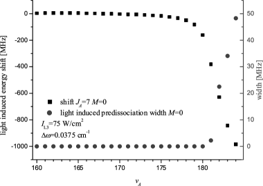
Figure 9: Simulation of light shifts and line broadenings of the last 25 vibrational levels of the $A^{1}\Sigma^{+}_{u}$ state calculated for $J_{A}\>$=7 and an intensity of the coupling laser of 75 W/cm². The coupling laser is assumed to be 0.0375 cm^-1 blue detuned to the atomic 3²p${}_{1/2}\rightarrow$ 3²d_3/2 transition. All levels of the A state are shifted to lower energies.

For the simulation of line shifts of asymptotic A state levels, we compare the theoretical energy positions of the single channel calculation of the A state with the corresponding values of the six channel system. A typical result of a simulation is presented in Figure 9. We display the energy shifts (squares) of vibrational levels $v_{A}=165,\dots,184$ with $J_{A}$=7 for a peak intensity of the coupling laser $I_{\rm L3}\>$= 75 W/cm² and a blue detuning of 0.0375 cm^-1 with respect to the atomic 3²P${}_{1/2}\rightarrow$ 3²D_3/2 transition. Moreover, the figure contains light induced line broadenings (circles) obtained from the simulations with imaginary absorbing potential. With the blue detuning of 0.0375 cm^-1 all levels bound by less than this energy starting with $v_{A}=181$ show considerable predissociation broadening of up to 49 MHz.

Similar calculations have been performed for all studied laser intensitites $I_{\rm L3}$ and detunings $\Delta\omega$ of the coupling laser. In Figure 10 the circles show a simulation of the dependence of level shifts for $v_{A}\>$=179, $J_{A}\>$=7 on the detuning $\delta\omega$ of the coupling laser with respect to a hypothetical transition ($v_{A}\>$=179, $J_{A}\>$=7)$\rightarrow$3s_1/2+3d_3/2 asymptote. Experimental points are plotted by squares.

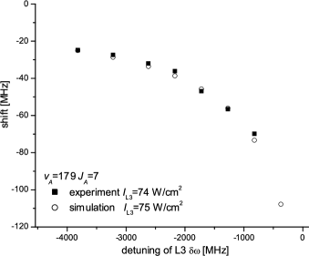
Figure 10: Dependence of the light shift of $v_{A}\>$=179, $J_{A}\>$=7 on the detuning of the coupling laser relative to a hypothetical transition ($v_{A}\>$=179, $J_{A}$=7)$\rightarrow$3s_1/2+3d_3/2 asymptote (see also Figure 7 and Figure 8). The squares are experimental points taken for a peak intensity of $I_{\rm L3}\>$=74 W/cm². The circles are from a simulation with $I_{\rm L3}\>$=75 W/cm².

The agreement between experimental and simulated line shifts is convincing, but one has to keep in mind that due to the uncertainty in the determination of the coupling laser beam waist, we have a 50% uncertainty in the laser intensities applied for the simulation. For detuning less than 1000 MHz our fitting procedure fails to determine line shifts from the experimental spectra. The experimental signal of the shifted trace decreases and broadens remarkably towards the resonance frequency. A typical spectrum showing this effect for $v_{A}=179$, $J_{A}=5,7$ is presented in Figure 11. The theoretical model applied for the fits of line profiles is no longer able to simulate the observed line profiles properly.

The deviations in Figure 11 are not noise; the slow variation is reproducible. For a proper simulation, the fit should include the fine and hyperfine structure on the optical coupling.

Figure 11: Example of an experimental scan of $v_{A}\>$=179, $J_{A}\>$=5,7 when the coupling laser is on resonance ($\delta\omega=0$) with respect to an hypothetical transition $v_{A}\>$=179, $J_{A}\>$=7$\rightarrow$3s_1/2+3d_3/2 asymptote. The intensity of L3 was $I_{\rm L3}$=74 W/cm². The dotted trace is taken without the coupling laser, while the dashed one is the manipulated spectrum. The solid traces represent fits on the experimental data with the model presented in Section 3.

A comparison of the line broadening observed in the experiment with theoretically predicted line broadening due to laser induced predissociation is shown in Figure 12. The experimental broadenings are calculated from the fitted FWHM in presence of the coupling laser minus the FWHM without light induced broadening. In the experiment we observe a significant line broadening, which has a maximum if the coupling laser is on resonance with a hypothetical transition frequency from the level under investigation to the 3s_1/2+3d_3/2 asymptote ($\delta\omega=0$). The broadening effect for $\delta\omega<0$ cannot be described by the laser induced predissociation calculated with our six channel model because the dissociation channel is not yet open.

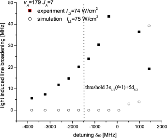
Figure 12: Dependence of the line broadening of $v_{A}=179$, $J_{A}=7$ on the detuning $\delta\omega$ of the coupling laser (see Figure 8). The squares represent the difference of the two FWHM fitting parameters. The circles are from a simulation for the experimental peak intensity of $I_{\rm L3}\>$=74 W/cm², neglecting the fine and hyperfine structure of the asymptote 3s+3d. The threshold is only given for the discussion in the text.

There are two different effects, which can lead to the experimentally observed line broadening for detuning $\delta\omega<0$. The molecular structure of the states at the 3s+3d asymptote is not as simple as we have assumed for the simulation. Due to the fine structure energy of the 3d atom and hyperfine energy of the 3s atom, which have almost the same magnitude ($E_{\rm FS}$(3d)=-0.0498 cm^-1 Bur87, $E_{\rm HFS}$(3s)=-0.0590 cm^-1 Ar77) the 3s+3d asymptote splits into four different hyperfine asymptotes. The calculated adiabatic asymptotic potentials are shown in Figure 13. From the A state, which correlates to the 3s${}_{1/2}(f=1)$+3p_1/2 asymptote, a dipole transition is only possible to the
3s${}_{1/2}(f=1)$+3d_3/2 asymptote. Thus, the light induced shifts of an asymptotic A state level shows a frequency dependence which can be described by an effective coupling to only this asymptote. In the region above the 3s${}_{1/2}(f=1)$+3d_5/2 asymptpote, which is the lowest asymptote due to the inverted fine structure, a predissociation can appear. This will lead to an increased line width of the A state levels under investigation starting at a detuning $\delta\omega>-|E_{\rm FS}|$. This threshold is included in Figure 12.

Figure 13: Hyperfine potentials at the asymptote $3s+3d$ for a total angular momentum $F=0$.

A second effect leading to a predissociation and thus a decreased lifetime of the 4${}^{1}\Sigma^{+}_{g}$ state is the vibrational coupling of this state to lower lying molecular states with the same symmetry. In Figure 14 the region of an avoided crossing with the 3${}^{1}\Sigma^{+}_{g}$-state is marked by a dashed box. The 3${}^{1}\Sigma^{+}_{g}$ state correlates to the 3s+4s asmyptote so that in the region above this asymptote a predissociation to this asymptote is possible. Therefore, the optical coupling of the A state to the 4${}^{1}\Sigma^{+}_{g}$-state can also induce a predissociation of A state levels to the 3s+4s asymptote.

Figure 14: Molecular potentials with ${}^{1}\Sigma^{+}_{g}$-symmetry. The shape of the 4${}^{1}\Sigma^{+}_{g}$-potential is due to an avoided crossing with the 3${}^{1}\Sigma^{+}_{g}$-state that correlates to the $3s+4s$ asympote Mag93.

Due to limitations of the memory available on our computers the two additional predissociation channels can not be implemented in our coupled channel code. Hence, it is difficult to estimate the contribution of the two effects to the experimentally observed line width.

6 Conclusion

A high resolution molecular beam experiment has been used to investigate the effect of a light induced coupling on the last vibrational levels of the sodium A state. The coupling is induced by a laser field which is near resonant to the atomic sodium 3²P${}_{1/2}\rightarrow 3^{2}$D_3/2 transition and thus couples the $A^{1}\Sigma^{+}_{u}$ state to the $4^{1}\Sigma^{+}_{g}$ and $2^{1}\Pi_{g}$ state, which are both correlated to the 3s_1/2+3d_3/2 asymptote. From the experimental data we see that with the usual laser intensities available from lab size laser sources ($\approx~{}50\;$W/cm²) light induced level shifts in a molecular system in the order of several 10 MHz can be induced. Furthermore, we observe an increased line width of the A state levels under investigation due to light induced predissociation. The number of bound states of the A state could be changed by the influence of the coupling laser by one or more units. Thus, in the picture of colliding atoms, the scattering phase was altered by more than $\pi$.

We developed a theoretical model of the light induced coupling, which describes the observed level shifts in good agreement with the experimental data. It is based on a six channel calculation using the Mapped Fourier Grid Method for the solution of the coupled channel eigenvalue problem. We use ab initio data for the electronic potentials at the 3s_1/2+3d_3/2 asymptote and for the dipole moments for the description of the light induced coupling. For the simulation of the induced line shifts of deeply bound states it is not necessary to take into account the fine and hyperfine structure of the 3s+3d asymptote.

The interpretation of the light induced line broadening effects needs a more detailed analysis of the molecular structure at the 3s+3d asymptote. The predissociation of the $4^{1}\Sigma^{+}_{g}$ and $2^{1}\Pi_{g}$ state due to fine structure, hyperfine structure, and vibrational motion must be taken into account.

This research is in progress with a similar experiment that couples the sodium ground state asymptote with the 3s+3p asymptote sam03. Here we want to investigate systematically a laser induced coupling between the X${}^{1}\Sigma^{+}_{g}$ ground state of sodium to levels in the A state. This experimental situation is of very high interest, as in most cooling and trapping experiments lasers (either for a MOT or dipole trap) are present, which are slightly detuned from the atomic resonance. These experiments show very complex dynamical Stark effect which asks for further extensions of our model system.

7 Acknowledgments

We thank the Deutsche Forschungsgemeinschaft supporting this work within the SFB 407. We also thank the PROCOPE program, which provided the money for the travelling expenses between France and Germany.