Finite nuclear size effect on Lamb shift of s_1/2, p_1/2, and p_3/2 atomic states

Abstract

We consider one-loop self-energy and vacuum polarization radiative corrections to the shift of atomic energy level due to finite nuclear size. Analytic expressions for vacuum polarization corrections are derived. For the self-energy of $p_{1/2}$ and $p_{3/2}$ states in addition to already known terms we derive next-to-leading nonlogarithmic $Z\alpha$-terms. Together with contributions obtained earlier the terms derived in the present work give explicit analytic expressions for $s_{1/2}$ and $p_{1/2}$ corrections which agree with results of previous numerical calculations up to Z=100 (Z is the nuclear charge number). We also show that the finite nuclear size radiative correction for a $p_{3/2}$ state is not small compared to the similar correction for a $p_{1/2}$ state at least for small $Z$.

I Introduction

Experimental and theoretical investigations of the radiative shift (Lamb shift) of energy levels in heavy atoms and ions is an important way to test Quantum Electrodynamics in the presence of a strong external electric field. One of the effects related to this problem is the dependence of the Lamb shift on the finite nuclear size (FNS). One can also look at this effect from another point of view. It is well known that there is an isotope shift of atomic levels due to the FNS. Corrections we are talking about are the radiative corrections to the isotope shift. There are two types of corrections. The first type is due to vacuum polarization and we will call them VPFNS corrections. The second type is due to the electron self-energy and vertex and we will call them SEVFNS corrections. Calculations of both VPFNS and SEVFNS corrections have attracted a lot of attention, for a review see Ref. MPS . Until recently it was mainly numerical work. The corrections for $1s$, $2s$, and $2p$ states have been calculated numerically, exactly in $Z\alpha$, in Refs.M ; JS ; CJS93 ; Mohr ; Blun ; LPSY ; BMPS ; see also review Borie for muonic atoms . Here $Z$ is the nuclear charge number and $\alpha$ is the fine structure constant. Analytical calculations have been based on $Z\alpha$-expansion. The s-wave VPFNS correction has been calculated a long time ago in order $\alpha(Z\alpha)$ F ; H . An ultraviolet logarithmic enhancement of higher order contributions to the VPFNS correction has been revealed in Ref. Mil0 . The enhancement factor is $\ln^{2}(\lambda_{C}/r_{0})$, where $\lambda_{C}$ is the Compton wave length and $r_{0}$ is the nuclear radius. In Ref. Mil0 the double-logarithmic contribution to the radiative correction to atomic parity nonconservation has been calculated analytically exactly in $Z\alpha$. The formula derived in Mil0 gives also one of the double-logarithmic contributions to the VPFNS correction for $s_{1/2}$ and $p_{1/2}$ states. The SEVFNS correction for an $s$-wave state has been calculated analytically in order $\alpha(Z\alpha)$ in Refs.Pach93 ; PG ; Mil ; Mil1 , see also reviews rev1 ; rev2 . Structure of higher-order contributions to the SEVFNS correction has been elucidated in our recent papers Mil ; Mil1 . The contributions are also logarithmically enhanced, but the enhancement factor contains only first power of $\ln(\lambda_{C}/r_{0})$. For $s_{1/2}$ and $p_{1/2}$ states prefactor before the logarithm has been calculated in Ref. Mil in order $\alpha(Z\alpha)^{2}$ and in Ref. Mil1 exactly in $Z\alpha$. Finally, contributions of the order $\alpha(Z\alpha)^{0}$ to SEVFNS corrections for $p_{1/2}$ and $p_{3/2}$ states have been calculated in recent papers Mil2 ; Jen .

In the present work we first calculate nonlogarithmic $\alpha(Z\alpha)$ terms of SEVFNS corrections for $p_{1/2}$ and $p_{3/2}$ states. Together with previously known contributions this gives a full analytic description for $p_{1/2}$ SEVFNS correction which agrees with previous numerical results up to $Z=100$. Our calculation demonstrates also that the $p_{3/2}$ SEVFNS correction is comparable with the $p_{1/2}$ SEVFNS correction. The second part of the work is devoted to analytical calculations of VPFNS corrections for $s_{1/2}$ and $p_{1/2}$ states. Analytic formulas obtained in this paper agree with previous numerical results up to $Z=100$.

The structure of the present paper is as follows. In Sec. II the general structure of SEVFNS and VPFNS corrections is discussed. In Sec. III we calculate $\alpha(Z\alpha)$ terms for $p_{1/2}$ and $p_{3/2}$ SEVFNS corrections, summarize all known terms for s-wave and p-wave corrections and compare analytic expressions with previous numerical results.In Sec. IV we first calculate unknown contributions to the VPFNS correction. Then we summarize contributions calculated in the present work and corrections obtained before and compare our analytic results with previous numerical calculations. Finally, Sec. V presents our conclusions.

II General structure of SEVFNS and VPFNS radiative corrections

Due to the finite nuclear size, the electric potential $V(r)$ of the nucleus differs from that for a point-like nucleus. The deviation is

$$\delta V(r)=V(r)-\left(-\frac{Z\alpha}{r}\right)$$ (1)

Throughout the paper we set $\hbar=c=1$. The diagram that describe the FNS effect in the leading order is shown in Fig.1a.

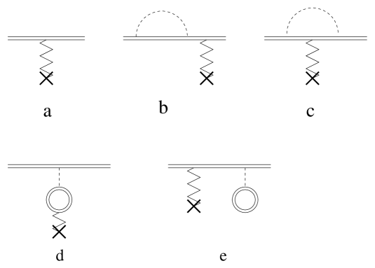
Figure 1: The leading contribution to the FNS effect is given by diagram (a), and one loop radiative corrections to the effect are given by diagrams (b-e). The double line denotes exact electron Green’s function in the Coulomb field of the nucleus, the cross denotes the nucleus, the zigzag line denotes the FNS perturbation (1), and the dashed line denotes the photon.

The double line corresponds to the exact electron wave function in the Coulomb field, the zigzag line with cross denotes the perturbation (1), and the dashed line denotes the photon. In momentum representation the perturbation (1) reads

$$\delta V(k)=\frac{4\pi Z\alpha}{k^{2}}[1-{\cal F}(k^{2})]\,,$$ (2)

where ${\cal F}(k^{2})$ is the nuclear form factor. An important fact is that (1) is a local interaction which is nonzero only at $r\sim r_{0}$, where $r_{0}$ is the nuclear radius. For estimates one can use the following formula for $r_{0}$

$$r_{0}\approx 1.1\ A^{1/3}\ fm\approx 1.5\ Z^{1/3}\ fm\ ,$$ (3)

where $A$ is the mass number of the nucleus. Dynamics of electrons at $r\sim r_{0}$ is ultrarelativistic at any value of $Z$. The Dirac wave function at $r\ll Z\alpha\lambda_{C}$ is of the form, see Ref. BLP

$$\Psi({\bm{r}})=Nr^{\gamma-1}\begin{pmatrix}(\kappa-\gamma)\Omega\\ iZ\alpha\tilde{\Omega}\end{pmatrix}\quad,$$ (4)

where $\Omega$ and $\tilde{\Omega}=-({\bm{\sigma}}\cdot{\bm{n}})\Omega$ are spherical spinors; $\kappa=-1$ for $s_{1/2}$ state, $\kappa=1$ for $p_{1/2}$ state, and $\kappa=-2$ for $p_{3/2}$ state; $\gamma=\sqrt{\kappa^{2}-(Z\alpha)^{2}}$; and $N$ is a constant known for each particular state. For hydrogenlike ions one can find $N$ using wave functions presented in Ref BLP . For multi-electron ions or atoms the constant $N$ can be calculated numerically. It can also be calculated analytically but in the semiclassical approximation Kh .

Due to ultrarelativistic nature of the problem the strong relativistic enhancement is a special property of SEVFNS and VPFNS radiative corrections. This is similar to atomic parity nonconservation (PNC) Kh . The relativistic enhancement factor for $s_{1/2}$ and $p_{1/2}$ states is proportional to $R_{rel}\sim(\lambda_{C}/Z\alpha r_{0})^{2(1-\gamma)}$, The factor is $R_{rel}\approx$3 for Cs and $R_{rel}\approx 9$ for Tl, Pb, and Bi Kh . The enhancement factor $R_{rel}$ is divergent at $r_{0}\to 0$. As a result behavior of SEVFNS, VPFNS, and PNC radiative corrections differs essentially from that of radiative corrections to the hyperfine structure.

The FNS energy shift $\Delta E$ in the leading approximation, diagram Fig.1a, has been calculated in numerous works both analytically and numerically. For a hydrogenlike ion there are simple parameterizations suggested in Ref. Shab

$$\Delta E_{ns_{1/2}} = \frac{Z^{2}}{10n}[1+(Z\alpha)^{2}f_{ns_{1/2}}]\left(\frac{2Z\alpha R}{n\lambda_{C}}\right)^{2\gamma}\ ,$$

$$\Delta E_{np_{1/2}} = \frac{Z^{4}\alpha^{2}(n^{2}-1)}{40n^{3}}[1+(Z\alpha)^{2}f_{np_{1/2}}]\left(\frac{2Z\alpha R}{n\lambda_{C}}\right)^{2\gamma}.$$ (5)

The energies are given in atomic units, $E_{0}=m\alpha^{2}=27.2eV$; $m$ is the electron mass; $n$ is the principal quantum number, $n=1,2,...$; $R\approx r_{0}$ is some effective radius (for details see Ref. Shab ); and coefficients $f_{i}=f_{i}(Z\alpha)$ are

$$f_{1s_{1/2}}(Z\alpha) = 1.380-0.162(Z\alpha)+1.612(Z\alpha)^{2}\ ,$$

$$f_{2s_{1/2}}(Z\alpha) = 1.508+0.215(Z\alpha)+1.332(Z\alpha)^{2}\ ,$$

$$f_{2p_{1/2}}(Z\alpha) = 1.615+4.319(Z\alpha)-9.152(Z\alpha)^{2}+11.87(Z\alpha)^{3}\ .$$ (6)

To be absolutely correct we should say that expectation values of the perturbation (1) taken with the wave functions (4) are not sufficient to calculate the energy shifts. One has also to take into account deformation of the wave function inside the nucleus. However, Eqs. (II) take this effect into account, and as soon as it is done there is no need to care about this detail any more.

Diagrams Fig.1(b-e) show the radiative corrections under discussion, see also comment com0 . Diagrams Fig.1b (self-energy) and Fig.1c (vertex) describe the SEVFNS correction and diagrams Fig.1d and Fig.1e describe the VPFNS correction. Note that Fig.1d corresponds to a modification of $\delta V$ (see Eq. (1)) due to the vacuum polarization, and Fig.1e corresponds to a modification of the electron wave function due to the vacuum polarization. Each of the diagrams Fig.1(b-e) gives some energy shift $\delta E_{i}$, i=b,c,d,e. Let us stress that for $s_{1/2}$ and $p_{1/2}$ states we always calculate a relative value of the radiative correction

$$\Delta_{s_{1/2}} = \delta E_{s_{1/2}}/\Delta E_{s_{1/2}}\ ,$$

$$\Delta_{p_{1/2}} = \delta E_{p_{1/2}}/\Delta E_{p_{1/2}}\ ,$$ (7)

where $\Delta E$ is the FNS shift given by diagram Fig.1a for the same atomic state. To find the value of $\Delta E$ one can use Eqs. (II), or a numerical calculation or any other method. Situation with $p_{3/2}$ correction is different and we discuss this at the end of section III (see Eq. (23). So, a crucially important point is that we calculate analytically only the relative quantity $\Delta$ . This is the central issue of this work as well as of our recent papers Mil0 ; Mil ; Mil1 ; Mil2 . The point is that convergence of $Z\alpha$-expansion for $\Delta$ is quite reasonable while the ultrarelativistic character of the FNS effect mentioned above makes the convergence of $Z\alpha$-expansion for $\delta E$ very poor. The good convergence of the series for the quantity $\Delta$ is related to separation of scales. Radiative corrections which do not contain $\ln(\lambda_{C}/r_{0})$ are related to quantum fluctuations at ”large” distances, $r\sim\lambda_{C}$. On the other hand, the perturbation is nonzero only at small distances $r\sim r_{0}\ll\lambda_{C}$. Therefore, the enhancement related to small distances in the contribution of ”large distance” quantum fluctuations is factorized similar to (II) , in essence this is a kind of effective operator approach. There are also quantum fluctuations from distances $r_{0}<r<\lambda_{C}$, their contribution cannot be trivially factorized and we take special care about these fluctuations. This is where terms dependent on $\ln(\lambda_{C}/r_{0})$ come from. The factorization of small distance enhancement in the part of the FNS effect related to the vacuum polarization was implicitly demonstrated in Ref. Lee .

III Self-energy and vertex FNS radiative corrections

Technically the most complicated are the self-energy and the vertex FNS radiative corrections (SEVFNS) given by diagrams in Fig.1b and Fig.1c. It has been demonstrated in paper Mil0 that relative SEVFNS corrections for $s_{1/2}$ and $p_{1/2}$ states are of the form

$$\Delta^{SEV}=\mathcal{A}\ln(b\lambda_{C}/r_{0})+\mathcal{B}\,,$$ (8)

where $\mathcal{A}$ and $\mathcal{B}$ are functions of $Z\alpha$ independent of $r_{0}$; $b=\exp(1/(2\gamma)-C-5/6)$, $\gamma=\sqrt{1-(Z\alpha)^{2}}$, $C\approx 0.557$ is the Euler constant. The function $\mathcal{A}(Z\alpha)$ is the same for $s_{1/2}$ and $p_{1/2}$ states. This function has been calculated in the leading order in $Z\alpha$ in Ref. Mil , the result reads

$$\mathcal{A}=-\frac{\alpha(Z\alpha)^{2}}{\pi}\left(\frac{15}{4}-\frac{\pi^{2}}{6}\right)\ .$$ (9)

It has been also calculated exactly in $Z\alpha$ in Ref. Mil1 . Plot of $\mathcal{A}$ from Ref. Mil1 is presented in Fig.2.

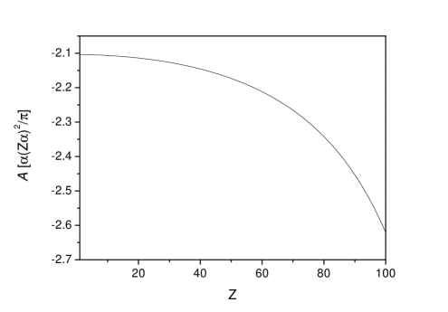
Figure 2: The function ${\cal A}$ , Eq.(8), calculated to all orders in $Z\alpha$. Value of the function is given in units $\alpha(Z\alpha)^{2}/\pi$.

Deviation of (9) from exact $\mathcal{A}(Z\alpha)$ is small even at $Z=100$. The function $\mathcal{B}(Z\alpha)$ for an $s_{1/2}$ state has been calculated in the leading order in $Z\alpha$ in Refs. Mil ; Mil1

$$\mathcal{B}_{s}=-\alpha(Z\alpha)\left(\frac{23}{4}-4\ln 2\right)\ .$$ (10)

It agrees numerically with earlier results Pach93 ; PG . Combining Eqs. (8),(9),(10) one gets the the following expression for s-wave SEVFNS correction

$$\Delta^{SEV}_{s_{1/2}}=-\alpha(Z\alpha)\left(\frac{23}{4}-4\ln 2\right)-\frac{\alpha(Z\alpha)^{2}}{\pi}\left(\frac{15}{4}-\frac{\pi^{2}}{6}\right)\ln(b\lambda_{C}/r_{0})\ .$$ (11)

The leading unaccounted term is of the order $\sim\alpha(Z\alpha)^{2}/\pi$. The correction (11) in % is plotted in Fig.3 by the dashed line. The same correction, but with $\mathcal{A}$ taken from Fig.2 is plotted in Fig.3 by the dotted line.

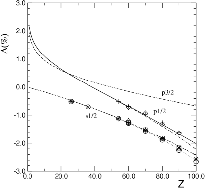
Figure 3: Relative SEVFNS corrections (%) for $s_{1/2}$ and $p_{1/2}$ states. The dashed line shows the correction $\Delta_{s_{1/2}}^{SEV}$ given by Eq. (11). The same correction, but with $\mathcal{A}$ taken from Fig.2 is plotted by the dotted line. Results of computations of $\Delta_{s_{1/2}}^{SEV}$ for $1s$ states are shown by squares CJS93 and stars Mohr . Similar results for $2s$ states are shown by triangles CJS93 and circles Mohr . The solid line shows the correction $\Delta_{p_{1/2}}^{SEV}$ given by Eqs. (8),(9),(21). The same correction, but with $\mathcal{A}$ taken from Fig.2 is plotted by the dashed-dotted line. Results of computations of $\Delta_{p_{1/2}}^{SEV}$ for $2p_{1/2}$ states are shown by diamonds CJS93 and crosses Mohr . The correction $\Delta_{p_{3/2}}^{SEV}$ given by Eq. (24) is plotted by the long-dashed line.

Our analytical results for $\Delta_{s_{1/2}}^{SEV}$ are in a good agreement with previous numerical data CJS93 ; Mohr shown by squares and stars for 1s state and by triangles and circles for 2s state. Some dependence of $\Delta_{s_{1/2}}^{SEV}$ on the principle quantum number $n$ can appear from function $\mathcal{B}_{s}$ in the order $\alpha(Z\alpha)^{2}/\pi$. However, one can see from the numerical data CJS93 ; Mohr presented in Fig. 3 that this dependence remains very weak up to $Z=100$.

The function $\mathcal{B}_{p1/2}$ for $p_{1/2}$ states in the leading order has been calculated in Refs. Mil2 ; Jen ,

$$\mathcal{B}_{p1/2}^{(0)}=\alpha\frac{8}{9\pi}\left(\ln\frac{1}{(Z\alpha)^{2}}+d\right)\ .$$ (12)

For $2p_{1/2}$ state the constant is $d=0.910$. This constant depends slightly on the principle quantum number $n$, see Ref. Jen .

It is interesting to note that $Z\alpha$-expansion of $\mathcal{B}_{p1/2}$ starts from $\alpha\ln(Z\alpha)$ term, while the same expansion for $\mathcal{B}_{s}$ starts from $\alpha(Z\alpha)$. It is related to a different infrared behavior of quantum fluctuations, see discussion in Ref. Mil2 .

Now we calculate the $\alpha(Z\alpha)$ term in the expansion of $\mathcal{B}_{p1/2}$. The electron wave function at small distances is given by Eq. (4). Let us first calculate the leading contribution to the FNS shift given by diagram in Fig.1a. For $s_{1/2}$ and $p_{3/2}$ states the upper component of the Dirac spinor (4) is much larger than the lower one. Hence, the upper component determines the FNS shift of such a state. On the other hand, for a $p_{1/2}$ state the lower component and hence its contribution to the FNS shift is dominating. A straightforward calculation gives the following values for the FNS shifts of $s$ and $p$ states (diagram Fig.1(a))

$$\Delta E_{ns_{1/2}} = \frac{2}{3n^{3}}(Z\alpha)^{4}m^{3}<r^{2}>\,,$$

$$\Delta E_{np_{1/2}} = \frac{n^{2}-1}{6n^{5}}(Z\alpha)^{6}m^{3}<r^{2}>\,,$$

$$\Delta E_{np_{3/2}} = \frac{n^{2}-1}{45n^{5}}(Z\alpha)^{6}m^{5}<r^{4}>\,.$$ (13)

Here $<r^{2}>$ and $<r^{4}>$ are values of $r^{2}$ and $r^{4}$ averaged over charge density of the nucleus, $n$ is the principle quantum number.

The low-momentum expansion of the nuclear electric form factor, see Eq. (2), is of the form

$${\cal F}(k^{2})\approx 1-\frac{k^{2}}{6}<r^{2}>+\frac{k^{4}}{120}<r^{4}>\,.$$ (14)

Modeling the nucleus as a uniformly charged ball one gets

$$<r^{2}>=\frac{3}{5}\ r_{0}^{2},\ \ \ <r^{4}>=\frac{3}{7}\ r_{0}^{4}\ .$$ (15)

As one should expect, the FNS corrections (III) obey the following inequalities $\Delta E_{s_{1/2}}\gg\Delta E_{p_{1/2}}\gg\Delta E_{p_{3/2}}$.

We consider now radiative corrections which originate from quantum fluctuations at distances $r\geq\lambda_{C}$. To calculate these ”soft” corrections it is sufficient to use nonrelativistic electron wave functions and, instead of (1), to use an effective FNS perturbation that reproduces the FNS correction $\Delta E_{ns1/2}$ for s-wave states, see Eq. (III) and Ref.Mil2 . The effective perturbation reads

$$\delta V_{eff}(r)=g\delta(\bm{r})\quad,\quad g=\frac{2\pi Z\alpha}{3}<r^{2}>\,.$$ (16)

In the leading approximation, SEVFNS corrections for $2p_{1/2}$ and $2p_{3/2}$ states, corresponding to diagrams Fig.1(b,c), have been calculated in Refs.Mil2 ; Jen :

$$\delta E^{(0)}_{2p_{1/2}}=F\left[\ln\frac{1}{(Z\alpha)^{2}}+0.910\right]\,,$$

$$\delta E^{(0)}_{2p_{3/2}}=F\left[\ln\frac{1}{(Z\alpha)^{2}}-0.215\right]\,,$$

$$where\ \ F=\frac{\alpha(Z\alpha)^{5}gm^{3}}{48\pi^{2}}\,.$$ (17)

These corrections are due to quantum fluctuations with the frequency $(Z\alpha)^{2}m\lesssim\omega\lesssim m$. Therefore, the effective operator is calculated with the relativistic effects taken into account. However, due to the behavior of the wave functions of $p$-states at $r\ll\lambda_{C}/(Z\alpha)$, it is possible to average this operator in the leading approximation over the nonrelativistic wave function. For $s$-states the situation is quite different LYE .

The ratio $\delta E^{(0)}_{2p_{1/2}}/\Delta E_{2p_{1/2}}$ defined by Eqs. (III) and (III) gives the relative correction (12). This means that Eqs. (III) correspond to zero order in $(Z\alpha)$-expansion of the function $\mathcal{B}_{p_{1/2}}$

We will see that next-order corrections $\delta E^{(1)}_{p_{1/2}}$ and $\delta E^{(1)}_{p_{3/2}}$ do not contain any logarithms, hence they come from quantum fluctuations at $r\sim\lambda_{C}$. Therefore it is convenient to calculate these corrections using the effective operator approach, see, e. g. Ref. rev1 . In this approach we first of all calculate scattering amplitude, described by diagrams shown in Fig.4.

Figure 4: Linear in $Z\alpha$ contributions to the electron scattering amplitude related to the p-wave SEVFNS correction. The solid line describes electron, the zigzag line denotes FNS perturbation (16), the dashed line denotes photon, and the cross denotes the nucleus. The diagrams with the permutation of Coulomb and perturbation lines should be added.

External electron momenta in Fig.4 are on mass shell and it is sufficient to consider scattering at low momenta $|\bm{p}_{1,2}|\ll m$. Here $\bm{p}_{1}$ and $\bm{p}_{2}$ are initial and final momenta of the electron, respectively. To find the energy shift one has to average the scattering amplitude over nonrelataivistic wave function of atomic electron. We have already used this technique to calculate (10) and to calculate a similar term for atomic parity nonconservation effect, see Refs. Mil ; Mil1 . Similar to these papers we use here the Fried-Yennie gauge Fried . One can find expressions for renormalized self-energy and vertex operators (ultraviolet renormalization) in this gauge in Refs.rev1 and Mil1 . However, the present calculation is more complicated than that in Mil ; Mil1 . The point is that in Refs. Mil ; Mil1 it was sufficient to calculate only the forward scattering amplitude, $\bm{p}_{1}=\bm{p}_{2}$. In the present case we have to consider scattering at arbitrary angle, $\bm{p}_{1}\neq\bm{p}_{2}$. It is not just a simple technical complication. The forward scattering amplitude is always infrared convergent. On the other hand the finite angle amplitude is always infrared divergent because of long range nature of the Coulomb field. To solve the problem we regularize the Coulomb interaction in Fig.4, $1/{\bm{k}}^{2}\rightarrow 1/({\bm{k}}^{2}+\lambda^{2})$, where $m\gg\lambda\gg|\bm{p}_{1,2}|$. Performing calculations we throw away all terms inversely proportional to $\lambda$ because they correspond not to the true radiative corrections, but just to Coulomb corrections to the scattering amplitude corresponding to Eqs. (III). Since we perform calculations in the Fried-Yennie gauge there is no need in an infrared regularization of non-Coulomb photon propagator in diagrams Fig.4. After a pretty long calculation we have found the following expressions for diagrams in Fig.4

$$M_{a} = G\left[\frac{7}{16}\,(\bm{\sigma}\cdot\bm{p}_{2})(\bm{\sigma}\cdot\bm{p}_{1})\right]\;,$$

$$M_{b}+M_{c} = G\left[-\left(\frac{5}{12}+\frac{4}{3}\ln 2\right)(\bm{\sigma}\cdot\bm{p}_{2})(\bm{\sigma}\cdot\bm{p}_{1})+\left(\frac{227}{192}-\frac{1}{3}\ln 2\right)(\bm{p}_{1}\cdot\bm{p}_{2})\right]\,,$$

$$M_{d} = G\left[\left(-\frac{1}{8}+\ln 2\right)(\bm{\sigma}\cdot\bm{p}_{2})(\bm{\sigma}\cdot\bm{p}_{1})-\left(\frac{61}{288}+\frac{8}{3}\ln 2\right)(\bm{p}_{1}\cdot\bm{p}_{2})\right]\ .$$ (18)

Here $\bm{\sigma}$ is the Pauli matrix, and $G=g\alpha(Z\alpha)/m^{2}$. Thus, the total scattering amplitude corresponding to Fig.4 reads

$$M=M_{a}+M_{b}+M_{c}+M_{d}=G\left[-\left(\frac{5}{48}+\frac{1}{3}\ln 2\right)(\bm{\sigma}\cdot\bm{p}_{2})(\bm{\sigma}\cdot\bm{p}_{1})+\left(\frac{559}{576}-3\ln 2\right)(\bm{p}_{1}\cdot\bm{p}_{2})\right]\,.$$ (19)

To find the effective Hamiltonian we transfer (19) to coordinate space using substitutions $(\bm{\sigma}\cdot\bm{p}_{2})(\bm{\sigma}\cdot\bm{p}_{1})\to(\bm{\sigma}\cdot\bm{p})\delta(\bm{r})(\bm{\sigma}\cdot\bm{p}),$ and $(\bm{p}_{1}\cdot\bm{p}_{2})\to(\bm{p}\,\delta(\bm{r})\bm{p}$) , where $\bm{p}=-i\nabla$. Finally, calculating expectation values of the effective Hamiltonian with the wave functions of $np$ states we obtain the following corrections to energy levels :

$$\delta E^{(1)}_{np_{1/2}} = F_{1}\left(\frac{379}{432}-\frac{16}{3}\ln 2\right)\ ,$$

$$\delta E^{(1)}_{np_{3/2}} = F_{1}\left(\frac{559}{432}-4\ln 2\right),$$

$$F_{1} = \frac{\alpha(Z\alpha)^{6}gm^{3}(n^{2}\!-\!1)}{4\pi n^{5}}\,.$$ (20)

Using $\delta E^{(0)}_{2p_{1/2}}$ from Eq. (III), $\delta E^{(1)}_{np_{1/2}}$ from Eq. (III), $\Delta E_{np_{1/2}}$ from (III) as well as definitions (II), (8) we find explicit expression for $\mathcal{B}_{p1/2}$ valid up to the first order in $(Z\alpha)$.

$$\mathcal{B}_{p1/2} = -\alpha\left[-\frac{8}{9\pi}\left(\ln\frac{1}{(Z\alpha)^{2}}+0.910\right)+(Z\alpha)\left(-\frac{379}{432}+\frac{16}{3}\ln 2\right)\right]\ .$$ (21)

Strictly speaking the constant near the logarithm depends on the principal quantum number. Equation (21) corresponds to the $2p_{1/2}$ state, for the $3p_{1/2}$ state one has to replace $0.910\to 0.908$, see Ref. Jen . Combining Eqs. (8),(9) and(21) one gets the the following expression for the SEVFNS radiative correction for a $p_{1/2}$ state

$$\Delta^{SEV}_{p_{1/2}}=\alpha\frac{8}{9\pi}\left(\ln\frac{1}{(Z\alpha)^{2}}+0.910\right)-\alpha(Z\alpha)\left(-\frac{379}{432}+\frac{16}{3}\ln 2\right)-\frac{\alpha(Z\alpha)^{2}}{\pi}\left(\frac{15}{4}-\frac{\pi^{2}}{6}\right)\ln(b\lambda_{C}/r_{0})\ .$$ (22)

The leading unaccounted term is of the order $\sim\alpha(Z\alpha)^{2}/\pi$. The correction (22) in % is plotted in Fig.3 by the solid line. The same correction, but with $\mathcal{A}$ taken from Fig.2 is plotted in Fig.3 by the dashed-dotted line. Our analytical calculation of $\Delta_{p_{1/2}}^{SEV}$ agrees very well with previous numerical results for $2p_{1/2}$ states shown by diamonds CJS93 and crosses Mohr , see also comment com1 .

Let us discuss now the SEVFNS correction for a $p_{3/2}$ state. In this case the definition (II) for the relative value of the correction is not sensible. The point is that according to (III) and (III) the SEVFNS correction $\delta E_{p_{3/2}}\propto\langle r^{2}\rangle$, and according to (III) the FNS correction $\Delta E_{p_{3/2}}\propto\langle r^{4}\rangle$. Therefore the definition (II) would imply that $\Delta_{p_{3/2}}\gg 1$. This itself is not a problem, just some rescaling. The real problem is that different powers of $r^{2}$ indicate that relativistic factors for $\delta E_{p_{3/2}}$ and $\Delta E_{p_{3/2}}$ are different. Therefore convergence of $(Z\alpha)$-expansion for $\Delta_{p_{3/2}}$ defined according to Eq. (II) must be very poor. Instead we define $\Delta_{p_{3/2}}$ as

$$\Delta_{np_{3/2}}=\delta E_{np_{3/2}}/\Delta E_{np_{1/2}}\ .$$ (23)

This is the ratio of the SEVFNS energy shift for $np_{3/2}$ state and the FNS energy shift for $np_{1/2}$ state. Using definition (23) we absorb all small-distance ($r\sim r_{0}$) effects into $\Delta E_{np_{1/2}}$, and therefore, according to the effective operator approach explained in section II, we expect a reasonable convergence of $(Z\alpha)$-expansion for $\Delta_{np_{3/2}}$. Using $\delta E^{(0)}_{2p_{3/2}}$ from Eq. (III), $\delta E^{(1)}_{np_{3/2}}$ from Eq. (III), $\Delta E_{np_{1/2}}$ from (III) as well as the definition (23) we obtain

$$\Delta_{p_{3/2}}^{SEV} = \alpha\frac{8}{9\pi}\left(\ln\frac{1}{(Z\alpha)^{2}}-0.215\right)-\alpha(Z\alpha)\left(-\frac{559}{432}+4\ln 2\right)\ .$$ (24)

Again, the constant near the logarithm depends on the principal quantum number. Equation (24) corresponds to the $2p_{3/2}$ state, for the $3p_{3/2}$ state one has to replace $-0.215\to-0.217$, see Ref. Jen . There are no $\ln(\lambda_{C}/r_{0})$ terms in $\Delta_{p_{3/2}}$, so the leading unaccounted term in (24) is of the order $\sim\alpha(Z\alpha)^{2}/\pi$. The correction $\Delta_{p_{3/2}}^{SEV}$ (%) given by Eq. (24) is plotted in Fig.3 by the long-dashed line. Note that it is comparable to $\Delta_{p_{1/2}}^{SEV}$. It means that absolute SEVFNS energy shifts $\delta E_{p_{3/2}}$ and $\delta E_{p_{1/2}}$ are also comparable.

IV Vacuum polarization FNS radiative corrections

In this section we consider vacuum polarization FNS radiative corrections (VPFNS) given by diagrams in Fig.1d and Fig.1e. Let us start from $s_{1/2}$ states. In the leading order in $(Z\alpha)$ the diagrams Fig.1d and Fig.1e can be represented as it is shown in Fig.5.

Figure 5: Linear in $Z\alpha$ FNS vacuum polarization corrections corresponding to $Z\alpha$-expansion of diagrams Fig.1d and Fig.1e. The solid line describes electron, the zigzag line denotes FNS perturbation (16), the dashed line denotes photon, and the cross denotes the nucleus.

Calculation of these diagrams for forward scattering $\bm{p}_{1}=\bm{p}_{2}$ is very simple, they give equal contributions, and their total contribution to the s-wave VPFNS correction is F ; H

$$\Delta^{VP(1)}_{s_{1/2}}=\frac{3}{4}\alpha(Z\alpha)\ .$$ (25)

Logarithmically enhanced contribution of diagram Fig.1e has been calculated in Ref.Mil0 , it reads

$$\Delta^{(e,log)}=\frac{2\alpha(Z\alpha)^{2}}{3\pi\gamma}\ln^{2}\left(\frac{b\lambda_{C}}{r_{0}}\right)\ .$$ (26)

This formula is equally valid for $s_{1/2}$ and $p_{1/2}$ states, for definition of parameters see Eq.(8). A logarithmically enhanced contribution of the diagram Fig.1d has not been calculated yet. A similar contribution has been estimated in Refs.Mil ; Mil1 in relation to atomic parity nonconservation (PNC). For PNC this contribution is strongly suppressed by the factor $1-4\sin^{2}\theta_{W}$, where $\theta_{W}$ is the Weinberg angle, therefore there have been no need in an accurate calculation. Now we perform an accurate calculation, the calculation is equally valid for $s_{1/2}$ and $p_{1/2}$ states.

According to (4) the electron density at $r\ll(Z\alpha)\lambda_{C}$ is

$$\rho(r)=Mr^{2(\gamma-1)}\ ,$$ (27)

where $M$ is some constant. Fourier transform of the density reads

$$\int e^{i\bm{k}\bm{r}}\,\rho(r)d\bm{r}=M\frac{4\pi}{k^{2\gamma+1}}\sin{(\pi\gamma)}\,\Gamma(2\gamma)\ ,$$ (28)

where $\Gamma(x)$ is the gamma function. Then, due to Eqs. (1) and (2) the FNS energy shift given by diagram Fig.1a reads

$$\Delta E=\int\delta V(r)\rho(r)d\bm{r}=M4Z\alpha\sin{(\pi\gamma)}\Gamma(2\gamma)r_{0}^{2\gamma}\int_{0}^{\infty}\frac{dy}{y^{\gamma+1}}[1-{\cal F}_{1}(y)]\,.$$ (29)

where $y=k^{2}r_{0}^{2}$, and ${\cal F}_{1}(y)={\cal F}(y/r_{0}^{2})$.

To generate diagram Fig.1d one has to account for the electron loop in the interaction energy (29). To do so we perform the following replacement in (29), see, e.g., Ref. rev1 and comment com2

$$\frac{1}{k^{2}}\to\frac{\alpha}{\pi m^{2}}\int_{0}^{1}dv\frac{v^{2}(1-v^{2}/3)}{4+(1-v^{2})k^{2}/m^{2}}\ .$$ (30)

This leads to the following expression for diagram Fig.1d

$$\delta E^{(d)}=M4Z\alpha\sin{(\pi\gamma)}\Gamma(2\gamma)r_{0}^{2\gamma}\int_{0}^{\infty}\frac{dy}{y^{\gamma+1}}[1-{\cal F}_{1}(y)]\,\,\frac{\alpha}{\pi}\int_{0}^{1}\frac{dv\,v^{2}(1-v^{2}/3)(y/a^{2})}{4+(1-v^{2})(y/a^{2})}\,,$$ (31)

where $a=mr_{0}=r_{0}/\lambda_{C}\ll 1$. Having in mind this inequality the expression (31) can be transformed to

$$\delta E^{(d)} = M4Z\alpha\sin{(\pi\gamma)}\Gamma(2\gamma)r_{0}^{2\gamma}\left(\frac{\alpha}{3\pi}\right)\left\{\int_{0}^{\infty}\frac{dy}{y^{\gamma+1}}[1-{\cal F}_{1}(y)]\left[\ln\frac{y}{a^{2}}-\frac{5}{3}\right]\right.$$ (32)

$$+ \left.\frac{3{\cal F}_{1}^{\prime}(0)\,a^{2(1-\gamma)}\,\pi^{3/2}4^{1-\gamma}\,\Gamma(\gamma+1)}{4(\gamma-1)\,\sin(\pi\gamma)\,\Gamma(\gamma+3/2)}\right\}\,,$$

where ${\cal F}_{1}^{\prime}(0)=\left.\frac{d{\cal F}_{1}}{dy}\right|_{y=0}$. Finally, introducing notation

$$J=\int_{0}^{\infty}\frac{dy}{y^{\gamma+1}}[1-{\cal F}_{1}(y)]\,,$$ (33)

and substituting Eqs. (32) and (29) in the definition (II) we obtain the following expression for logarithmically enhanced contribution to the relative correction corresponding to Fig.1d

$$\Delta^{(d,log)}=\left(\frac{\alpha}{3\pi}\right)\left\{\left[2\ln\frac{\lambda_{C}}{r_{0}}-\frac{5}{3}-\frac{\partial\,\ln J}{\partial\gamma}\right]+\frac{3{\cal F}_{1}^{\prime}(0)(\lambda_{C}/r_{0})^{2(1-\gamma)}\,\pi^{3/2}4^{1-\gamma}\,\Gamma(\gamma+1)}{4(\gamma-1)\,\sin(\pi\gamma)\,\Gamma(\gamma+3/2)\,J}\right\}\,.$$ (34)

This formula is equally valid for $s_{1/2}$ and $p_{1/2}$ states.

For large $Z$, as soon as $(1-\gamma)\ln(\lambda_{C}/r_{0})\gg 1$, the ${\cal F}_{1}^{\prime}$-term in (34) can be neglected and

$$\Delta^{(d,log)}\to\left(\frac{\alpha}{3\pi}\right)\left[2\ln\frac{\lambda_{C}}{r_{0}}-\frac{5}{3}-\frac{\partial\,\ln J}{\partial\gamma}\right]\ .$$ (35)

A similar high $Z$ estimate has been used in Mil ; Mil1 . For small $Z$, more precisely for $(1-\gamma)\ln(\lambda_{C}/r_{0})\ll 1$, the correction behaves as

$$\Delta^{(d,log)}\to\frac{\alpha(Z\alpha)^{2}}{3\pi}\ln^{2}\left(\frac{\lambda_{C}}{r_{0}}\right)\,.$$ (36)

The simplest way to obtain this limiting behavior is to expand intermediate expressions (29) and(31), however, one can also obtain the same result expanding the exact answer (34).

Behavior of the exact expression (34) between asymptotical regimes (35) and (36) depends on the particular form factor $F$. However, the dependence is pretty weak, and for further analysis we use the form factor of uniformly charged ball of radius $r_{0}$.

$$F(y)=\frac{3}{y}\left[\frac{\sin\sqrt{y}}{\sqrt{y}}-\cos\sqrt{y}\right]$$ (37)

An explicit integration in (33) gives

$$J=\frac{6\cos(\pi\gamma)\Gamma(-1-2\gamma)}{3+2\gamma}\,,$$

$$-\frac{\partial\ln J}{\partial\gamma}=\pi\tan(\pi\gamma)+\frac{2}{3+2\gamma}+2\psi(-1-2\gamma)\,,$$ (38)

where $\psi(x)=d\ln\Gamma(x)/dx$. Combining together Eqs. (25), (26), (34), (IV), as well as unaccounted in the present calculation correction $u(Z\alpha)\sim\alpha(Z\alpha)^{2}/\pi$ we obtain the following expression for the total vacuum polarization correction for s-electron

$$\Delta^{VP}_{s_{1}/2} = \frac{3}{4}\alpha(Z\alpha)+\frac{2\alpha(Z\alpha)^{2}}{3\pi\gamma}\ln^{2}\left(\frac{b\lambda_{C}}{r_{0}}\right)$$ (39)

$$+ \left(\frac{\alpha}{3\pi}\right)\left\{\left[2\ln\frac{\lambda_{C}}{r_{0}}-\frac{5}{3}+\pi\tan(\pi\gamma)+\frac{2}{3+2\gamma}+2\psi(-1-2\gamma)\right]\right.$$

$$- \left.\frac{\pi^{3/2}4^{(1-\gamma)}(3+2\gamma)\Gamma(\gamma+1)}{40\sin(2\pi\gamma)(\gamma-1)\Gamma(-1-2\gamma)\Gamma(\gamma+3/2)}\left(\frac{\lambda_{C}}{r_{0}}\right)^{2(\gamma-1)}\right\}+u(Z\alpha)\,.$$

The correction (39) with $u(Z\alpha)=0$ is plotted in Fig.6a by the solid line. Results of computations of the same correction performed in Ref JS for $1s$ states are shown by squares and for $2s$ states are shown by triangles. Agreement between our analytical calculation and JS ) is pretty good. Moreover, we can determine $u(Z\alpha)$ fitting the numerical data. Result of the fit reads

$$u=2.5\frac{\alpha(Z\alpha)^{2}}{\pi}\ .$$ (40)

The correction (39) with $u(Z\alpha)$ given by (40) is plotted in Fig.6a by the dashed line.

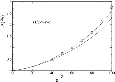
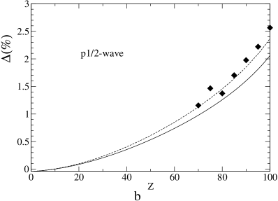
Figure 6: Relative VPFNS corrections (%) for $s_{1/2}$ and $p_{1/2}$ states. The solid line in Fig. “a” shows the correction $\Delta_{s}^{VP}$ given by Eq. (39) with $u(Z\alpha)=0$. The dashed line shows the same correction with $u(Z\alpha)$ given by Eq. (40). Results of computations JS are shown by squares for $1s$ states and by triangles for $2s$ states. The solid line in Fig. “b” shows the correction $\Delta_{p_{1/2}}^{VP}$ given by Eq. (43) with $u(Z\alpha)=0$. The dashed line shows the same correction with $u(Z\alpha)$ given by Eq. (40). Results of computations JS for $2p_{1/2}$ states are shown by diamonds.

Let us consider now the VPFNS correction for a $p_{1/2}$ state. Logarithmically enhanced contributions (26) and (34) are exactly the same as for $s_{1/2}$ states. There is also a contribution of zero order in $(Z\alpha)$ calculated in Mil2

$$\Delta^{VP(0)}_{p_{1/2}}=-\frac{8}{45\pi}\alpha\ .$$ (41)

To calculate the first order correction we once more employ the effective operator approach and consider the scattering amplitude described by Fig.5, in this case ${\bm{p}}_{1}\neq{\bm{p}}_{2}$. Similar to the procedure described in Section III we regularize the Coulomb interaction in Fig.5, $1/{\bm{k}}^{2}\rightarrow 1/({\bm{k}}^{2}+\lambda^{2})$, where $m\gg\lambda\gg|\bm{p}_{1,2}|$. Performing calculations we throw away all terms inversely proportional to $\lambda$ because they correspond not to true radiative corrections, but just to Coulomb corrections to scattering amplitude corresponding to Eq. (41). Then we obtain the following result for the first-order correction

$$\Delta^{VP(1)}_{p_{1/2}}=\frac{23}{72}\alpha(Z\alpha)\ .$$ (42)

The coefficient is $23/72=1/8+7/36$, where the first term comes from the diagram Fig.5e, and the second term comes from the diagram Fig.5d. Combining together Eqs. (41), (42), (26), (34), (IV), as well as unaccounted in the present calculation correction $u(Z\alpha)\sim\alpha(Z\alpha)^{2}/\pi$ we obtain the following expression for total vacuum polarization correction for a $p_{1/2}$ state

$$\Delta^{VP}_{p_{1/2}} = -\frac{8}{45\pi}\alpha+\frac{23}{72}\alpha(Z\alpha)+\frac{2\alpha(Z\alpha)^{2}}{3\pi\gamma}\ln^{2}\left(\frac{b\lambda_{C}}{r_{0}}\right)$$ (43)

$$+ \left(\frac{\alpha}{3\pi}\right)\left\{\left[2\ln\frac{\lambda_{C}}{r_{0}}-\frac{5}{3}+\pi\tan(\pi\gamma)+\frac{2}{3+2\gamma}+2\psi(-1-2\gamma)\right]\right.$$

$$- \left.\frac{\pi^{3/2}4^{(1-\gamma)}(3+2\gamma)\Gamma(\gamma+1)}{40\sin(2\pi\gamma)(\gamma-1)\Gamma(-1-2\gamma)\Gamma(\gamma+3/2)}\left(\frac{\lambda_{C}}{r_{0}}\right)^{2(\gamma-1)}\right\}+u(Z\alpha)\,.$$

In principle the unaccounted contribution $u(Z\alpha)$ can be different from that in (39). The correction (43) with $u(Z\alpha)=0$ is plotted in Fig.6b by a solid line. Results of computations of $\Delta^{VP}_{p_{1/2}}$ performed in Ref JS for $2p_{1/2}$ states are shown by diamonds. Once more, the agreement is pretty good. We also find unknown $u(Z\alpha)$ fitting the numerical data JS . The fit gives the result very close to that for s-wave, see Eq. (40). The dashed line in Fig.6b shows the correction (43) with $u(Z\alpha)$ given by Eq. (40).

Finally we consider the VPFNS correction for a $p_{3/2}$ state, the relative correction is defined according to Eq. (23). There is a contribution of zero order in $(Z\alpha)$ calculated in Mil2

$$\Delta^{VP(0)}_{p_{3/2}}=-\frac{8}{45\pi}\alpha\ .$$ (44)

It is equal to that for a $p_{1/2}$ state, see Eq. (41). The first-order correction is given by diagrams in Fig.5. The calculation of the correction, which is similar to the calculation of (42), gives

$$\Delta^{VP(1)}_{p_{3/2}}=\frac{5}{72}\alpha(Z\alpha)\ .$$ (45)

This correction comes from the diagram Fig.5d only. There are no logarithmically enhanced contributions to $\Delta^{VP}_{p_{3/2}}$, therefore with accuracy $\sim\alpha(Z\alpha)^{2}/\pi$ accepted in the present work the correction $\Delta^{VP}_{p_{3/2}}$ is given by sum of (44) and (45)

$$\Delta^{VP}_{p_{3/2}}=-\frac{8}{45\pi}\alpha+\frac{5}{72}\alpha(Z\alpha)\ .$$ (46)

V Summary and conclusions

In the present work we have calculated analytically the finite nuclear size effect on Lamb shift of $s_{1/2}$, $p_{1/2}$, and $p_{3/2}$ atomic states. Corresponding radiative corrections are strongly affected by ultrarelativistic behavior of electrons in the vicinity of the nucleus. As a result of this behavior the convergence of $Z\alpha$-expansion is very poor for absolute energy shifts, and on the other hand the convergence is reasonably good for relative corrections which we consider. We define the relative corrections for $s_{1/2}$ and $p_{1/2}$ states according to Eq. (II), and for $p_{3/2}$ states according to Eq. (23). The self-energy and vertex finite size (SEVFNS) relative radiative correction for a $s_{1/2}$ state is given by Eq. (11). The SEVFNS correction for a $p_{1/2}$ state is given by Eq. (22), and the SEVFNS correction for a $p_{3/2}$ state is given by Eq. (24). The vacuum polarization finite size (VPFNS) relative radiative correction for a $s_{1/2}$ state is given by Eqs. (39),(40). The VPFNS correction for a $p_{1/2}$ state is given by Eqs. (43),(40), and the VPFNS correction for a $p_{3/2}$ is given by Eq. (46). Our analytical results for $s_{1/2}$ and $p_{1/2}$ states agree well with previous numerical calculations.

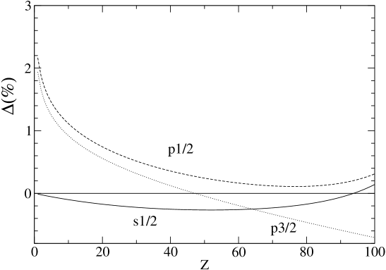
Figure 7: Total (SEVFNS + VPFNS) finite size relative radiative corrections (%) for $s_{1/2}$ (solid line), $p_{1/2}$ (dashed line), and $p_{3/2}$ (dotted line) states.

Finally, in Fig. 7 we plot the total radiative corrections which include self-energy, vertex and vacuum polarization diagrams (SEVFNS + VPFNS). For $s_{1/2}$ and $p_{1/2}$ states at large $Z$ there are strong compensations between SEVFNS and VPFNS contributions. We would like to attract attention to the $p_{3/2}$ correction. The same normalization is used for $p_{1/2}$ and $p_{3/2}$ states. Therefore, from Fig. 7 we come to a somewhat paradoxical conclusion that at large $Z$ the finite nuclear size effect on Lamb shift of $p_{3/2}$ states is larger than that for $p_{1/2}$ states. Moreover, using Fig. 7 and Eqs. (II) we conclude that at large $Z$ the finite nuclear size effect on Lamb shift of $p_{3/2}$ states is only by a few times smaller than that for $s$ states. These conclusions are not consistent with numerical data JS at large $Z$. Certainly, our calculation for $p_{3/2}$ states is valid only up to the order $\alpha(Z\alpha)$. The $p_{3/2}$ correction does not contain the ultraviolet logarithm and therefore the convergence of $Z\alpha$-expansion can be different from that for $s_{1/2}$ and $p_{1/2}$ states. A poor convergence of the expansion could be the reason for disagreement with previous numerical calculatins. However a new exact in $Z\alpha$ numerical calculation for $p_{3/2}$ states would be interesting.

We are grateful to G. Soff for helpful comments. The work was supported by RFBR grants 01-02-16926 and 03-02-16510.

References

- (1) P. J. Mohr, G. Plunien, and G. Soff, Phys. Rep. 293, 227 (1998).
- (2) P. J. Mohr, At. Data Nuc. Data Tables 29, 453 (1983).
- (3) W. R. Johnson and G. Soff, At. Data Nuc. Data Tables 33, 405 (1985).
- (4) K. T. Cheng, W. R. Johnson, and J. Sapirstein, Phys. Rev. A 47, 1817 (1993).
- (5) P. J. Mohr and G. Soff, Phys. Rev. Lett., 70, 158 (1993).
- (6) S. A. Blundell, Phys. Rev. A 46, 3762 (1992).
- (7) I. Lindgren, H. Persson, S. Salomonson, A. Ynnerman, Phys. Rev. A 47, 4555 (1993).
- (8) T. Beier, P. J. Mohr, H. Persson, and G. Soff, Phys. Rev. A 58, 954 (1998).
- (9) E. Borie and G. A. Rinker, Rev. Mod. Phys. 54, 67 (1982).
- (10) J. L. Friar, Z. Phys. A 292, 1 (1979); 303. 84(E) (1981).
- (11) D. J. Hylton, Phys. Rev. A 32, 1303 (1985).
- (12) A. I. Milstein and O. P. Sushkov, Phys. Rev. A 66, 022108 (2002).
- (13) K. Pachucki, Phys. Rev. A 48, 120 (1993).
- (14) M. I. Eides , H. Grotch, Phys. Rev. A 56, R2507 (1997).
- (15) A. I. Milstein, O. P. Sushkov and I. S. Terekhov, Phys. Rev. Lett., 89, 283003 (2002).
- (16) A. I. Milstein, O. P. Sushkov and I. S. Terekhov, Phys. Rev. A 67, 062103 (2003).
- (17) M. I. Eides , H. Grotch, and V. A. Shelyuto, Phys. Rep. 342, 63 (2001).
- (18) J. L. Friar, nucl-th/0211064.
- (19) A. I. Milstein, O. P. Sushkov, I. S. Terekhov, Phys. Rev. A 67, 062111 (2003).
- (20) U. D. Jentschura, J. Phys. A: Math. Gen. 36, L229 (2003).
- (21) V. B. Berestetskii, E. M. Lifshitz, and L. P. Pitaevskii, Relativistic quantum theory (Pergamon Press, Oxford, 1982).
- (22) Parity nonconservation in atomic phenomena, I. B. Khriplovich, Gordon and Breach, 1991.
- (23) V. M. Shabaev, J. Phys. B 26, 1103 (1992).
- (24) Except of diagrams shown in Fig. 1 there is also a contribution related to normalization of the bound state wave function (a ”derivative term”). This term is not important for calculations performed in the present work. However, it is important for calculations performed in our previous papers Mil ; Mil1 results of which we use here. The “derivative term” has been taken into account in Mil ; Mil1 .
- (25) R. N. Lee and A. I. Milstein, Phys. Lett. A 189, 72 (1994).
- (26) G.P.Lepage, D.R.Yennie, and G.W. Erickson, Phys. Rev. Lett.47, 1640 (1981).
- (27) H. M. Fried, D. R. Yennie, Phys. Rev. , 1391 (1958).
- (28) In the previous work Mil2 we found the -term in Eqs. (21),(22) by fitting numerical data CJS93 ; Mohr . As a result of the fit we got . According to the calculation performed in the present work the exact result reads .
- (29) In this work we do not consider Wichmann-Kroll corrections. These corrections to the induced-charge density related to the FNS effect were considered in Lee .