Statistical properties of transport in plasma turbulence

Abstract

The statistical properties of the $E\times B$ flux in different types of plasma turbulence simulations are investigated using probability density distribution functions (PDF). The physics included in the models ranges from two dimensional drift-wave turbulence to three dimensional MHD simulations. The PDFs of the flux surface averaged transport are in good agreement with an extreme value distribution (EVD). This is interpreted as a signature of localized vortical structures dominating the transport on a flux surface. Models accounting for a local input of energy and including the global evolution of background profiles show a more bursty behaviour in 2D as well as 3D simulations of interchange and drift type turbulence. Although the PDFs are not Gaussian, again no algebraic tails are observed. The tails are, in all cases considered, in excellent agreement with EVDs.

, , ,

1 Introduction

In hot magnetised plasmas the main cross-field transport is often found to be far larger than expected for diffusive transport due to collisions. In plasma physics the transport is then called anomalous while in fluid dynamics ”strange” or ”anomalous” transport signifies the non-diffusive character of the transport. We investigate the statistical properties of the turbulent particle flux with the aim to examine the anomality of the transport in the fluid sense of meaning. An important feature stressed by many authors is the non-Gaussianty of the PDF of the point-wise measured flux [1, 2, 3, 4]. While the non-Gaussianity of the flux PDF is to be expected from a quantity that itself is a folding of two statistical variables, namely density and radial velocity, the observation of power law tails in the flux PDF would be an indication of anomalous transport in the fluid sense of the wording, that is non-diffusive transport behaviour. Correspondingly this would indicate the presence of long range correlations in the turbulence [5]. Experimental results showing finite size scaling and similarity of transport PDFs measured in different experimental devices have recently been reported in Refs. [6, 7]. These measurements have shown that transport in the edge and scrape-off layer (SOL) region of fusion devices is highly intermittent, self similar and does in its statistical features not vary much between machines of different sizes and geometries. A characteristic feature of the transport seems to be the non-Gaussianity observed in its PDF and its intermittency. Intermittent transport would indicate that indeed the particle transport is anomalous not only in the sense that it is not due to collisions, but also in the sense that it is non-diffusive. A non-diffusive transport, however, has distinct scaling properties, which would pose much stricter conditions on the design of the vessel surrounding a fusion device, as this has to withstand the largest likely transport event. Additionally, a number of fundamental questions in relation to transport PDFs are still unanswered, so it is as yet unclear what ingredients are needed to produce a certain transport PDF. Are transport PDFs dependent on the driving mechanism behind the turbulence? How does different physics enter into the transport PDF? Here we present initial answers to some of these questions by analysing direct numerical simulations of various types of plasma turbulence in different geometries.

2 Local turbulence Models

In this section we consider plasma turbulence in a classical sense, namely as being based on a scale separation between the equilibrium and fluctuations, f.x. density fluctuations are assumed small compared the the equilibrium density $\tilde{n}/n_{00}<<1$. The fluid equations for drift micro-turbulence result from standard ordering based upon the slowness of the dynamics compared to the ion gyro-frequency $\Omega_{i}=eB/M_{i}$ and hence the smallness of the drift scale $\rho_{s}$ compared to the background pressure gradient scale length $L_{\perp}$. These quantities and the sound speed $c_{s}$ are defined by

$$\Omega_{i}={eB\over M_{i}},\qquad c_{s}^{2}={T_{e}\over M_{i}},\qquad\rho_{s}={c_{s}\over\Omega_{i}},\qquad L_{\perp}=\left|\nabla\log p_{e}\right|^{-1},$$ (1)

where subscripts $e$ and $i$ refer to electrons and ions respectively, and the temperature is given in units of energy. Normalization is in terms of scaled dependent variables (electrostatic potential $e\phi/T_{e}$, electron density $n/n_{00}$, parallel ion velocity $u/c_{s}$, parallel electric current $J/n_{00}ec_{s}$; respectively). In addition the dependent quantities are scaled with the small parameter $\delta=\rho_{s}/L_{\perp}$, so that we calculate with quantities of order one. The quantity $n_{00}$ is a normalizing density, while $n_{0}(x)$ is the equilibrium plasma density having a finite gradient. In normalized units the radial profile of the density is $\partial_{r}\log n_{0}(x)=-1$. Vorticity is defined via $\omega=\nabla_{\perp}^{2}\phi$.

2.1 Two dimensional drift turbulence

Assuming electrostatic motion, neglecting eletron inertia and replacing parallel derivatives by an effective parallel wavelength $L_{\shortparallel}$ we arrive at the well known Hasegawa-Wakatani equations [8] (HWE), describing two dimensional drift-wave turbulence in the absence of magnetic field line curvature:

$$\partial_{t}\omega+\{\varphi,\omega\}=-\frac{1}{L_{\|}^{2}\nu}\left(n-\varphi\right)+\mu_{\omega}\nabla^{2}\omega,$$ (2)

$$\partial_{t}n+\{\varphi,n\}+\partial_{y}\varphi=-\frac{1}{L_{\|}^{2}\nu}\left(n-\varphi\right)+\mu_{n}\nabla^{2}n\;,$$ (3)

where the Poisson bracket ${\left\{f,g\right\}}={\partial f\over\partial x}{\partial g\over\partial y}-{\partial f\over\partial y}{\partial g\over\partial x}$ is used to write the non-linear terms originating from advection with the $E\times B$ drift velocity. In this system the turbulence is driven by the resistive instability. We solve the HWE on a double periodic domain [9] and typically we use $256\times 256$ modes on a square of side length $L=40$. To produce self-consistent stationary turbulence we start the simulations from low amplitude ($10^{-6}$) random density fluctuations and initialise all other fields to zero. The fluctuations grow due to the resistive instability and saturate with amplitudes of order one. After saturation [10] we measure the local turbulent radial particle transport ($x$-direction) as given in a single point:

$$\Gamma_{n,\mbox{loc}}=nv_{r}\;,$$ (4)

and the flux surface averaged flux $\Gamma_{n,\mbox{FS}}$:

$$\Gamma_{n,\mbox{FS}}=\frac{1}{L_{y}}\int_{0}^{L_{y}}\Gamma_{n,\mbox{loc}}\;dy\;,$$ (5)

which in the two dimensional context is trivially obtained by averaging over the poloidal coordinate $y$. Density and potential fluctuations have PDFs that are well described by Gaussians. Consequently the PDF of the $E\times B$ flux, $\Gamma_{n,\mbox{loc}}$, as depicted in Fig. 2, is close to the functional form expected from the folding of Gaussian PDFs for the density fluctuations $n$ and the radial $E\times B$-velocity, $v_{r}=-\partial_{y}\phi$ [4]:

$$P_{\mbox{FG}}(\Gamma)=\frac{1}{\pi}\frac{\sqrt{1-c^{2}}}{\sigma_{n}\sigma_{v_{r}}}K_{0}\left(\frac{|\Gamma|}{\sigma_{n}\sigma_{v_{r}}}\right)\exp\left(-c\frac{\Gamma}{\sigma_{n}\sigma_{v_{r}}}\right)\;.$$ (6)

where $c$ is the correlation between density and radial velocity fluctuations $c=-\frac{\langle v_{r}n\rangle}{\langle v_{r}^{2}\rangle^{1/2}\langle n^{2}\rangle^{1/2}}=\cos{\alpha_{nv_{r}}}$, $K_{0}$ is the modified Bessel function of second kind, and $\alpha_{nu}$ is the phase angle between $n$ and $v_{r}$. Furthermore we have $\sigma_{v_{r}}\equiv\langle v_{r}^{2}\rangle^{1/2}(1-c^{2})^{1/2}\;,$ and correspondingly for $\sigma_{n}$.

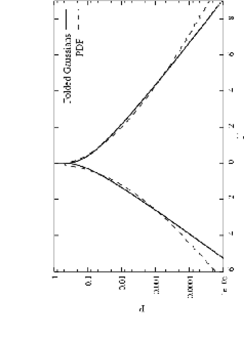
Figure 1: PDF of $\Gamma_{n,\mbox{loc}}$ compared with folded Gaussian

Figure 2: PDF of $\Gamma_{n,\mbox{FS}}$, compared to an EVD a log-normal distribution and a Gaussian

Using Eq.(3) for an approximate relationship between density and potential and the drift-wave dispersion relation to lowest orderin the long-wavelength limit $\omega=\frac{k_{y}}{1+k_{\perp}^{2}}$ , we find:

$$\Gamma_{n,\mbox{\small FS}}=-\frac{1}{L_{y}}\int_{0}^{L_{y}}n\partial_{y}\phi\;dy\approx\frac{L_{\|}^{2}\nu}{L_{y}}\int_{0}^{L_{y}}\left(\partial_{y}\nabla_{\perp}\phi\right)^{2}\;dy\geq 0\,.$$ (7)

Thus the flux surfaced averaged transport is to lowest order positive definite, as confirmed by the numerical simulations. It is thus the PDF of the logarithm of the transport, $\ln\Gamma_{n,\mbox{\small FS}}$, that converges towards a Gaussian, if the central limit theorem applies. As seen from Fig. 2 the transport PDF of $\Gamma_{n,\mbox{\small FS}}$ is indeed very well described by a log-normal distribution with in the present case zero offset $z=0$:

$$P_{\mbox{\small ln}}(\Gamma)=\frac{1}{\sqrt{2\pi}\sigma}\frac{1}{\Gamma-z}\exp\left(-\frac{1}{2}\left(\frac{\ln(\frac{\Gamma-z}{m})}{\sigma}\right)^{2}\right)\;.$$ (8)

An alternative description of the statistical properties of the flux can be made in terms of the extreme value distribution (EVD). For a statistical variable – here the averaged flux – that is dominated by the minimum or maximum of a large number of random observations – here the local flux events – the EVD arises[11]:

$$P_{\mbox{\small EVD}}(\Gamma)=\frac{1}{g}\exp\left(-\frac{\Gamma-h_{0}}{g}\right)\exp\left[-\exp\left(-\frac{\Gamma-h_{0}}{g}\right)\right]\,.$$ (9)

The EVD has recently been used successfully to model and explain statistical properties of electron pressure fluctuations in a non-confinement plasma experiment [12]. As seen from Fig. 2 the EVD explains the observed transport PDF in this case as well as the lognormal distribution and is indistinguishable from the former. One should, however, note that the EVD decays faster than the lognormal one and, thus, is better suited to describe statistical variables that are limited not only from below, but also from above. Clearly the maximum transport event in all real world systems is limited by the system size. We interpret the present situation in the sense that the flux surface averaged transport is dominated by extreme events, probably mediated by transport events linked to vortical structures. The flux PDF itself in this case is naturally skewed, but the radial particle transport is by no means ’strange’ in the sense of not being diffusive on large time and space scales. No power law tail is observed in the data. That indeed the transport is diffusive is augmented by the fact, that the radial dispersion of ideal test-particles in 2D Hasegawa-Wakatani turbulence is found to be asymptotically diffusive as well [13, 14].

2.2 Drift-Alfvén and MHD turbulence

Next we consider electromagnetic drift-Alfvén turbulence with magnetic field curvature effects. The geometry is a three dimensional flux tube with local slab-like coordinates $\left[x,y,s\right]$ [15] and the model is defined by the temporal evolution of the following four scalar fields: electrostatic potential $\phi$, density $n$ given by electron density continuity equation, parallel current $J$, and parallel ion velocity $u$, with the parallel magnetic potential $A_{\parallel}=-\nabla_{\perp}^{-2}J$:

$${\partial\omega\over\partial t}+{\bf v}_{E}\cdot\nabla\omega={K}\left(n\right)+\nabla_{\|}J+\mu_{w}\nabla_{\perp}^{2}\omega\,,$$ (10)

$${\partial n\over\partial t}+{\bf v}_{E}\cdot\nabla(n_{0}+n)={K}\left(n-\phi\right)+\nabla_{\|}\left(J-u\right)+\mu_{n}\nabla_{\perp}^{2}n\,,$$ (11)

$${\partial\over\partial t}\left(\hat{\beta}A_{\parallel}+\hat{\mu}J\right)+\hat{\mu}{\bf v}_{E}\cdot\nabla J=\nabla_{\|}\left(n_{0}+n-\phi\right)-CJ\,,$$ (12)

$$\hat{\epsilon}\left({\partial u\over\partial t}+{\bf v}_{E}\cdot\nabla u\right)=-\nabla_{\|}\left(n_{0}+n\right)\,.$$ (13)

The advective and parallel derivatives carry non-linearities entering through $\phi$ and $A_{\parallel}$: ${\bf v}_{E}\cdot\nabla=\{\phi,\},$ and $\nabla_{\parallel}={\partial\over\partial s}-\{\hat{\beta}A_{\parallel},\}$. Finally, the curvature operator ${K}=-\omega_{B}\left(\sin s\partial_{x}+\cos s\partial_{y}\right)$ originates from compressibility terms. The parameters in the equations reflect the competition between parallel and perpendicular dynamics, reflected in the scale ratio $\hat{\epsilon}=(qR/L_{\perp})^{2}$. The electron parallel dynamics is controlled by

$$\hat{\beta}={2\mu_{0}p_{e}\over B^{2}}\,\hat{\epsilon}\,,\qquad\qquad\hat{\mu}={m_{e}\over M_{i}}\,\hat{\epsilon}\,,\qquad\qquad C=0.51{L_{\perp}\over\tau_{e}c_{s}}\hat{\mu}=\nu\hat{\mu}\,,$$ (14)

where $\tau_{e}$ is the electron collision time and the factor $0.51$ reflects the parallel resistivity [16]. The competition between these three parameters, representing magnetic induction, electron inertia, and resistive relaxation determines the response of $J$ to the force imbalance in Eq. (12). The simulations are performed on a grid with $64\times 256\times 16$ points and dimensions $64\times 256\times 2\pi$ in ${x,y,s}$. Some runs were repeated with double resolution to ensure convergence. Standard parameters for the runs were $\hat{\mu}=5$, $\hat{s}=1$, $\omega_{B}=0.05$ with the viscosities set to $\mu_{w}=\mu_{n}=0.025$.
A transition in the dynamical behaviour from drift-Alfvén to turbulence dominated by MHD modes is in this model triggered by increasing the ratio of $\hat{\beta}/\hat{\mu}$. To check the nature of the observed turbulence we evaluate the phase shift $\alpha$ between density and potential fluctuations in dependence of $k_{y}$ using the relationship $\alpha_{k_{y}}=\log{I}(\phi_{k_{y}}n_{k_{y}}^{*})$. For better statistics the phase is averaged along the parallel coordinate $s$ and time.

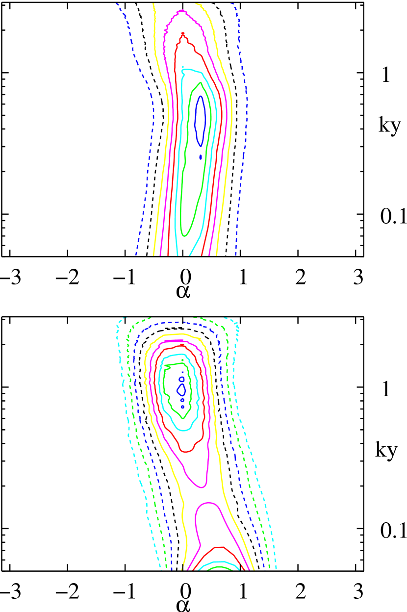
Figure 3: Probability of phase angle $\alpha$ between density and potential fluctuations for $\hat{\beta}=0.5$ (top) and $\hat{\beta}=50$ (bottom) versus $k_{y}$.

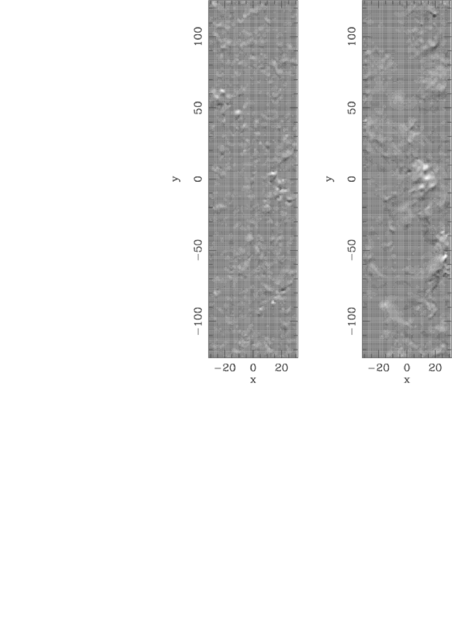
Figure 4: Spatial structure of the transport $\Gamma_{n,\mbox{loc}}$ at the for $\hat{\beta}=0.5$ (left) and $\hat{\beta}=50$ (right).

Fig. 4 shows for a low value $\hat{\beta}=0.5$ and a high value $\hat{\beta}=50$ the change in principal behaviour of the turbulence with increasing $\hat{\beta}$. A shift towards larger phase angles is observed for low $k_{y}$-modes indicating the transition from drift-Alfvén to MHD type of turbulence. As the turbulence character changes to become more of the MHD type the phase relationship between density and potential is altered. This is also reflected in a visual inspection of the spatial transport structure (Fig. 4). It shows that the transport for high values of $\hat{\beta}$ is carried by larger structures than for low $\hat{\beta}$. The local flux $\Gamma_{n,\mbox{loc}}$ has the interesting structure that outward (white) and inward (dark) transport regions are closely related, this reflects the fact that the transport is carried in localized structures, having an outward flux at the one side and an inward flux at the other side. They are linked to corresponding eddies in the vorticity field.
In both regimes the turbulence decreases the equilibrium density gradient by about $5-10\%$ in the stationary turbulence, a further deviation from the background density gradient is prevented by a feed-back mechanism in two damping layers at the inner and outer radial boundary, which drive the flux-surface averaged density towards the initially specified values. The PDFs of transport related quantities for $\hat{\beta}=0.5$ and $\hat{\beta}=50$ are shown in Figs. 6 and 6.

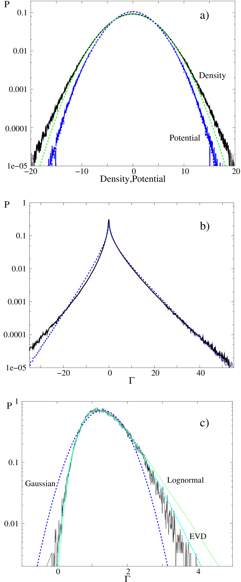
Figure 5: Low $\hat{\beta}=0.5$ case. a) PDF’s for density $n$ and potential $\phi$ fluctuations with fitted Gaussians (dashed) b) $\Gamma_{n,\mbox{loc}}$ with fitted folded Gaussian c) $\Gamma_{n,\mbox{FS}}$ with a fitted Gaussian, log-normal and extreme value distribution (EVD).

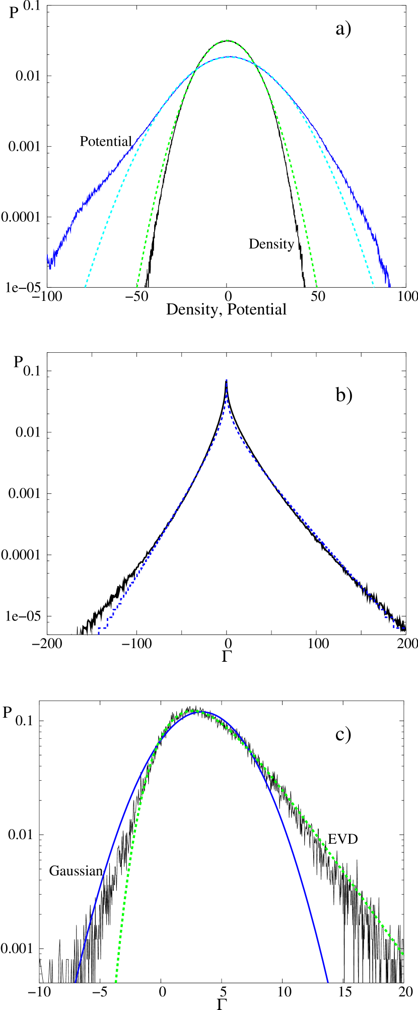
Figure 6: High $\hat{\beta}=50$ case. a) PDF’s for density $n$ and potential $\phi$ fluctuations with fitted Gaussians (dashed) b) $\Gamma_{n,\mbox{loc}}$ with fitted folded Gaussian and c) $\Gamma_{n,\mbox{FS}}$ with a fitted Gaussian and extreme value distribution (EVD). The log-normal distribution is not shown, as it is very close to the EVD.

In the low beta case density and potential fluctuations have PDFs that are very well described by Gaussians, with minor deviations from Gaussianity in the tails. Density and potential have a rather similar PDF as they are well correlated and consequently the fitted folded Gaussian $P_{FG}$ Eq. (6) describes rather well the point-wise flux PDF ($c=0.2$) . An indication of a power-law tail in the point-wise flux PDF is not observed, and the point-wise flux PDF decays exponentially. The PDF of the magnetic flux surface averaged density flux $\Gamma_{n,\mbox{FS}}$, shown in Fig. 6 c), is much closer to a shifted Gaussian, depicted for comparison in the figure, but we observe a “fat-tail” towards larger transport events. However, the flux surface averaged particle flux will, even though not positive definite, be at least limited from below, with excursions to a negative averaged flux being unlikely. Thus in Fig. 6 c) we also present the fitted log-normal distribution, with parameters $\sigma=0.273$, $z=-9.3$, and $m=11$. This fits the data well, but over-predicts the tail, an indication of the fact that the transport is limited from above as well, as we are considering a finite system. Indeed the EVD with parameters $h_{0}=2.60$ and $g=0.34$ fits the data very well, especially the tail of the PDF. For the MHD situation with $\hat{\beta}=50$ — even though the phase relation between density and potential differs and the turbulence has different character — we observe transport statistics similar to the drift-Alfvén case. The corresponding PDFs for this case are depicted in Fig. 6. As the density and potential fluctuations are less well coupled in that regime the PDFs of density and potential differ more. The potential fluctuations also deviate more from a Gaussian. Compared to the density fluctuations they now have a larger width. Note that the fluctuation level has increased significantly as well as the transport level when compared to the low beta case. Nevertheless the PDF of the point-wise measured transport is still well described by a folded Gaussian as seen in Fig. 6 b. The flux surface averaged transport is shown in comparison with a fitted EVD and a Gaussian. The log-normal distribution function is not plotted here, as it is very close to the EVD. The flux surface averaged transport behaviour has changed little as compared to the low beta case. It is still much closer to an EVD (or log-normal) than to a Gaussian one, however, we observe that to the low transport side the Gaussian distribution fits the transport PDF better. This effect is due to enhanced levels of small noisy transport events occurring in the MHD type of simulation and the flux PDF is more influenced by these small scale “random” transport events. Their distribution centers around zero, while the large scales reproduce the global transport PDF and carry the net flux. The small scale transport events then make an appearance in the transport PDF for small averaged fluxes, which explains the nearly Gaussian behaviour of the flux PDF on the low transport side.

3 Global Models

After having considered local models we now drop the scale separation between turbulent fluctuations and equilibrium — or in the cases where no equilibrium exists, as in the SOL, between fluctuations and time averaged background. A motivation for this is that in the edge the fluctuation level is of the same order of magnitude as the background and going out into the SOL region the fluctuations in density can actually exceed the average density by a large factor. However, regarding fluctuations and background on the same footing requires that the system is integrated to much longer times and thus higher demands in terms of computational power. We thus consider a two dimensional and a simple three dimensional model.

3.1 Flute Model

Concerning only two dimensional dynamics of the plasma is – if at all – only a good approximation in the SOL. We here consider a newly developed global interchange model for the full particle density $n$, temperature $T$ and vorticity $\omega$, with ${d=\over dt}\partial_{t}+\frac{\hat{z}\times\nabla\phi\cdot\nabla}{B}$:

$${dn\over dt}+n{K}(\phi)-{K}(n) = \mu_{n}\nabla_{\perp}^{2}n+S_{n}-\sigma_{n}(n-1)$$ (15)

$$\frac{3}{2}{dT\over dt}+T{K}(\phi)-\frac{7}{2}T{K}(T)-\frac{T^{2}}{n}{K}(n) = \mu_{T}\nabla_{\perp}^{2}T+S_{T}-\frac{3}{2}\sigma_{T}(T-1)$$ (16)

$$\left(\partial_{t}+\hat{z}\times\nabla\phi\cdot\nabla\right)\omega-{K}(p) = \mu_{\omega}\nabla_{\perp}^{2}\omega-\sigma_{\omega}\omega\;.$$ (17)

Here the coupling between the equations is exclusively due to the curvature operator $K=\zeta\partial/\partial y$ where $\zeta=2\rho_{s}/R_{0}$ with $R_{0}$ the radius of curvature of the toroidal magnetic field. The coupling due to parallel currents giving rise to drift-wave dynamics is absent from these equations.

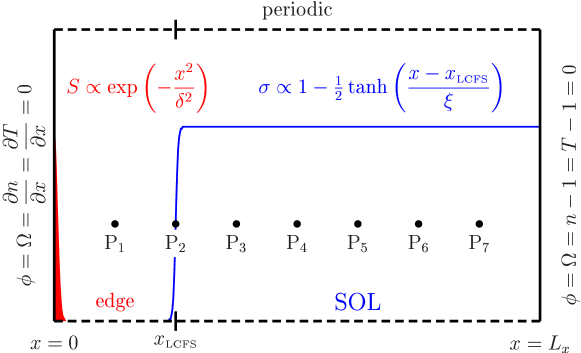
Figure 7: Geometry showing shape of source and sink terms and the locations were long timeseries are taken.

The $S$-terms on the right hand sides represent sources of particles and heat, while the $\sigma$-terms operating in the SOL (Fig. 7) are sinks due to the parallel loss to end plates along open field lines. Boundary conditions correspond to free-slip, while in normalized units $n=T=1$ at $x=L_{x}$ and $\partial n/\partial x=\partial T/\partial x=0$ at $x=0$, see Fig.7. For strong forcing the system is unstable to interchange modes causing significant convective transport. A novel property of this model is the non-linear conservation of the energy integral $E=\int d\bm{x}\,\left[\frac{1}{2}\left(\nabla\phi\right)^{2}+\frac{3}{2}\,nT\right]$, revealing the conservative transfer of energy from thermal to kinetic form due to magnetic field curvature. A realistic modeling of this process is mandatory for predictive global models. Nevertheless the solutions for strong forcing shows the characteristic “on-off” character of the turbulence due to self-sustained sheared flows [17]. The time-averaged thermal gradients are strongest in the source regions and are “flapping” back and forth, leading to intermittent ejection of particles and heat far out into the SOL region.

Figure 8: PDF of pointwise and flux surface averaged transport inside LCFS and in the SOL

The transport PDF obtained from direct numerical simulation of that model is very different from the ones obtained for the fluctuation based model. The flux surface averaged transport is no longer constant and instead varies with radial position as density is lost in the parallel direction. We here take the transport data from a long timeseries since it is impossible to use spatial homogeneity in the radial direction to increase the quality of the statistics. It here makes sense to compare flux PDF’s by normalising them to their root mean square. Fig. 8 shows the PDFs of the point-wise and the flux-surface averaged transport at radial positions corresponding to the edge and the SOL part of the simulation domain, ($P_{1}$ and $P_{4}$ in Fig. 7). A slight tendency to larger flux events in the SOL is observed. Averaging the transport poloidally has less dramatic effects than for the models considered in Section 2. The reason for this is the large poloidal correlation lengths of the order of the poloidal size of the simulation domain.

Figure 9: Tail of the flux surface averaged transport in the SOL (see Fig. 8) fitted with an EVD.

Figure 10: Flux surface and time averaged transport in the SOL fitted with an EVD and a power law.

Fig. 10 demonstrates that even for this obviously highly intermittent and bursty transport the EVD ($h_{0}=1.35$ and $g=0.60$ ) is an excellent fit for the tail of the PDF. However, if the data are additionally averaged over times longer than the times between bursts, we observe a behaviour that can as well be approximated by a power law PDF as an EVD (Fig. 10). The amount of data being in the tail is small in that case, and the data-range is about 1.5 decades in $\Gamma$ and down from six to only two decades in the ordinate (Fig. 10). One should note that whenever the variance of the data is large the body of a EVD will be similar to a straight line in a log-log plot, while its tail decays with increasing slope in the log-log plot. This shows the danger of fitting a PDF only for a very limited range in a doubly logarithmic plot. Our interpretation is thus, that to observe a distinct behaviour of the tail of the transport PDF one needs to be able to fit data over at least two decades and that fitting data on smaller regions is highly arbitrary and not suited to distinguish between different interpretations of the data.

3.2 Electrostatic Drift Model

Finally we consider a three dimensional global version of drift-wave equations. The model uses quasi-neutrality and electron density continuity, together with the parallel force balance equations for ions and electrons. Parallel convection is kept. No assumptions are made on the scale length of the background gradient compared to the fluctuation scales, e.g. the constraint $\nabla n_{0}\sim\nabla\tilde{n}\sim\epsilon\ll 1$ as underlying f.x. the HWE Eqs.: (2) and (3) is dropped. The resulting system is written in terms of the logarithm of density $N=\log(n)$:

$${d\omega\over dt}+\nabla N\cdot\frac{d}{dt}\nabla\phi = \mu_{\omega}\nabla^{2}\omega+\nabla_{\|}(U-V)+(U-V)\nabla_{\|}N$$ (18)

$${dN\over dt} = -\left(V\nabla_{\|}N+\nabla_{\|}V\right)+\mu_{n}\left(\nabla^{2}N+(\nabla N)^{2}\right)$$ (19)

$${dU\over dt} = -\nabla_{\|}\phi-\nu_{e,i}U$$ (20)

$${dV\over dt} = \frac{M}{m_{e}}\nabla_{\|}\left(\phi-N\right)-\left(\nu_{ei}+\nu_{e,n}\right)V$$ (21)

The energetic coupling is due to the parallel current dynamics that is by the difference in parallel electron velocity $V$ and parallel ion velocity $U$. Now coupling due to curvature is absent from the equations. Again, the density is the full density evolving and is fed into the system on the inner side, while on the radially outer third of the system Bohm-sheath boundary conditions are implemented. The inner two thirds of the radius have periodic boundary conditions in the parallel direction. The $y$-direction is periodic and fixed values are imposed on field quantities at the outer radial boundary, while the diffusive fluxes are set to zero at the inner radial boundary by prescribing a zero radial gradient there. The system is solved on a 128x64x30 grid. Due to the heavy computational load of that system it could not be integrated to times as high as the 2D system, which influences the quality of the statistics.

Figure 11: PDF of flux surface averaged transport in the edge (left) with fitted EVD on bulk and tail of distribution and in the SOL (right) with EVD fitted on the tail of the distribution.

The flux PDF in this case shows distinct differences between edge region (closed field lines) and SOL with open field lines and losses to the limiter plates. For the edge region the poloidal correlation length is shorter than the box length and thus the PDF of the averaged transport is similar to that of the 2D- and 3D drift wave model. It fits well with an EVD in the tail and in the bulk (see Fig. 11). The flux PDF in the SOL part of the domain bears the characteristics of long poloidal correlations observed in that regime, due to the flute modes – rather than drift waves – dominating the dynamics in the SOL. Thus the shape of the transport PDF, also after flux surface averaging, is very similar to that of the interchange model (see. Figs. 8 and 10), demonstrating also the applicability of 2D models in the SOL. However, the tail of the PDF again does not show any sign of a power law behaviour and can over the whole range be fitted very well with an EVD.

4 Conclusion

Direct numerical simulations of physically distinct models of flute and drift modes in two and three dimensional geometries have been presented and analysed in terms of the transport PDF. For the fluctuation based models non-linear structures in the plasma dominate the transport, but give rise to a diffusive turbulent transport rather than a super-diffusion or otherwise anomalous (in the fluid sense) transport. Consequently a Gyro-Bohm like scaling of the transport with the magnetic field is found. Similar behaviour has recently been reported in investigations on test particle transport in plasma turbulence [14, 18].
There is little difference in the results concerning different physical models. If the energy input into the system is changed from a homogeneous input due to a local, fixed pressure gradient to a localized plasma source and sink regions are added the transport PDF becomes more bursty and longer poloidal correlations arise. Also in this situation the tails of all flux PDFs considered are extremely well fitted by extreme value distributions. Thus, the deviation of the point-wise as well as the flux surface averaged flux from Gaussianity is, at least in the asymptotic limit of large system size, not due to anomalous — in the sense of non-diffusive — behaviour. The presented observations should not be interpreted as indicators for the presence of self organized criticality. An interpretation in terms of occurrence of extreme transport events, which may be caused by localized eddies seems to be more appealing. The statistics describing the transport PDF should therefor be taken from extreme value statistics, which in all cases fits the tails of the observed transport PDF very well.

References

- [1] T. Huld, S. Iizuka, H. L. Pécseli, J. J. Rasmussen, Experimental investigation of flute-type electrostatic turbulence, Plasma Phys. Contr. Fusion 30 (10) (1988) 1297 – 1318.
- [2] T. Huld, A. H. Nielsen, H. L. Pécseli, J. J. Rasmussen, Coherent structures an 2-dimensional plasma turbulence, Phys. Fluids B 3 (7) (1991) 1609 – 1625.
- [3] M. Endler, H. Niedermeyer, L. Giannone, E. Holzauer, A. Rudyj, G. Theimer, N. Tsois, Asdex-Team, Measurements and modelling of electrostatic fluctuations in the scrape-off layer od asdex, Nuclear Fusion 35 (1995) 1307–1339.
- [4] B. A. Carreras, C. Hidalgo, E. Sánchez, M. Pedrosa, R. Balbín, García-Cortés, B. van Milligen, D. E. Newman, V. E. Lynch, Fluctuation induced flux at the plasma edge in toroidal devices, Phys. Plasmas 3 (1996) 2664–2672.
- [5] G. M. Zaslavsky, Chaos, fractional kinetics, and anomalous transport, Phys. Rep. 371 (2002) 461 – 580.
- [6] B. A. Carreras, V. E. Lynch, B. LaBombard, Structure and properties of the electrostatic fluctuations in the far scrape-off layer region of alctor c-mod, Phys. Plasmas 8 (8) (2001) 3702 – 3707.
- [7] C. Hidalgo, B. Goncalves, M. A. Pedrosa, J. Castellano, K. Erents, A. L. Fraguas, M. Hron, J. A. Jimenez, G. F. Matthews, B. van Milligen, C. Silva, Empirical similarity in the probability density function of turbulent transport in the edge plasma region in fusion plasmas, Plasma Phys. Contr. Fusion 44 (8) (2002) 1557 – 1564.
- [8] M. Wakatani, A. Hasegawa, A collisional drift wave description of plasma edge turbulence, Phys. Fluids 27 (1984) 611–618.
- [9] V. Naulin, A. H. Nielsen, J. Juul Rasmussen, Dispersion of ideal particles in a two-dimensional model of electrostatic turbulence, Phys. Plasmas 6 (1999) 4575 – 4585.
- [10] V. Naulin, Aspects of flow generation and saturation in drift-wave turbulence, New J. Phys. 4 (2002) 28.
- [11] D. Sornette, Critical Phenomena in Natural Sciences, Springer, Berlin, 2000.
- [12] K. Rypdal, S. Ratynskaia, Statistics of low-frequency plasma fluctuations in a simple magnetized torus, Phys. Plasmas 10 (2003) 2686.
- [13] R. Basu, T. Jessen, V. Naulin, J. Juul Rasmussen, Turbulent flux and the diffusion of passive tracers in electrostatic turbulence, Phys. Plasmas 10 (7) (2003) 2696–2703.
- [14] R. Basu, V. Naulin, J. Juul Rasmussen, Particle diffusion in anisotropic turbulence, Comm. in Nonlinear Science and Numerical Simulation 8 (2003) 477–492.
- [15] B. D. Scott, Shifted metric procedure for flux tube treatments of toroidal geometry: Avoiding grid deformation, Phys. Plasmas 8 (2) (2001) 447 – 458.
- [16] S. I. Braginskii, Transport processes in a plasma, in: M. A. Leontovich (Ed.), Reviews of Plasma Physics, Consultants Bureau, New York, 1965.
- [17] O. E. Garcia, V. Naulin, A. H. Nielsen, J. Juul Rasmussen, Fluctuation statistics from numerical simulations of scrape-off layer turbulence, submitted to: Phys. Rev. Letters .
- [18] Z. Lin, S. Ethier, T. S. Hahm, W. M. Tang, Phys. Rev. Lett, 88 (2002) 195004–1.