Optically bound microscopic particles in one dimension

Abstract

Counter-propagating light fields have the ability to create self-organized one-dimensional optically bound arrays of microscopic particles, where the light fields adapt to the particle locations and vice versa. We develop a theoretical model to describe this situation and show good agreement with recent experimental data (Phys. Rev. Lett. 89, 128301 (2002)) for two and three particles, if the scattering force is assumed to dominate the axial trapping of the particles. The extension of these ideas to two and three dimensional optically bound states is also discussed.

I Introduction

The ability of light to influence the kinetic motion of microscopic and atomic matter has had a profound impact in the last three decades. The optical manipulation of matter was first seriously studied by Ashkin and co-workers in the 1970s Ashkin1 ; Ashkin2 ; Ashkin3 , and led ultimately to the demonstration of the single beam gradient force trap Ashkin4 , referred to as optical tweezers, where the gradient of an optical field can induce dielectric particles of higher refractive index than their surrounding medium to be trapped in three dimensions in the light field maxima Ashkin4 . Much of Ashkin’s early work centered not on gradient forces, but on the use of radiation pressure to trap particles Ashkin1 , and a dual beam radiation pressure trap was demonstrated in a which single particle was confined. This work ultimately contributed to the development of the magneto-optical trap for neutral atoms Chu .

Recently we observed one-dimensional arrays of silica spheres trapped in a dual beam radiation pressure trap Sveta . These arrays had an unusual property in that the particles that formed the array were regularly spaced from each other. The particles were redistributing the incident light field, which in turn redistributed the particle spacings, allowing them to reside in equilibrium positions. This effect, known as “optically bound matter” was first realised in a slightly different context via a different mechanism to ours some years ago Burns ; Burns1 using a single laser beam and was explained as the interaction of the coherently induced dipole moments of microscopic spheres in an optical field creating bound matter.

In the context of our study optically bound matter is of interest as it relates to the way in which particles interact with the light field in extended optical lattices, which may prove useful for the understanding of three-dimensional trapping of colloidal particles vanB . Indeed optically bound matter may provide an attractive method for the creation of such lattices that are not possible using interference patterns. Bound matter may also serve as a test bed for studies of atomic or ionic analogues to our microscopic system Blatt .

Subsequent to our report a similar observation was made in an experiment making use of a dual beam fiber trap Singer . In this latter paper a theory was developed that examined particles of approximately the same size as the laser wavelength involved. In this paper we develop a numerical model that allows us to simulate the equilibrium positions of two and three particles in a counter-propagating beam geometry, where the particle sizes are larger than the laser wavelength, and fall outside the upper bound of the limits discussed in Singer . The model can readily be extended to look at larger arrays of systems. We discuss the role of the scattering and refraction of light in the creation of arrays. In the next section we describe the numerical model we use for our studies and derive predictions for the separation of two and three spheres of various sizes. We then compare this with both previous and current experiments.

II Theory Section

Our model comprises two monochromatic laser fields of frequency $\omega$ counter-propagating along the z-axis which interact with a system of $N$ transparent dielectric spheres of mass $m$, refractive-index $n_{s}$, and radius $R$, with centers at positions $\{\vec{r}_{j}(t)\},j=1,2,\ldots N$, and which are immersed in a host medium of refractive-index $n_{h}$. The electric field is written

$$\vec{E}(\vec{r},t)=\frac{\hat{\bf e}}{2}\left[({\cal E}_{+}(\vec{r})e^{ikz}+{\cal E}_{-}(\vec{r})e^{-ikz})e^{-i\omega t}+c.c\right],$$ (1)

where $\hat{\bf e}$ is the unit polarization vector of the field, ${\cal E}_{\pm}(\vec{r})$ are the slowly varying electric field amplitudes of the right or forward propagating $(+)$ and left or backward propagating $(-)$ fields, and $k=n_{h}\omega/c$ is the wavevector of the field in the host medium. The incident fields are assumed to be collimated Gaussians at longitudinal coordinates $z=-L/2$ for the forward field and $z=L/2$ for the backward field

$${\cal E}_{+}(x,y,z=-L/2)={\cal E}_{-}(x,y,z=L/2)=\sqrt{\frac{4P_{0}}{n_{h}c\epsilon_{0}\pi w_{0}^{2}}}e^{-r^{2}/w_{0}^{2}},$$ (2)

where $r^{2}=x^{2}+y^{2}$, $w_{0}$ is the initial Gaussian spot size, and $P_{0}$ is the input power in each beam. It is assumed that all the spheres are contained between the beam waists within the length $L>>R$.

Consider first that the dielectric spheres are in a fixed configuration at time $t$ specified by the centers $\{\vec{r}_{j}(t)\}$. Then the dielectric spheres provide a spatially inhomogeneous refractive index distribution which can be written in the form

$$n^{2}(\vec{r})=n_{h}^{2}+(n_{s}^{2}-n_{h}^{2})\sum_{j=1}^{N}\theta(R-|\vec{r}-\vec{r}_{j}(t)|),$$ (3)

where $\theta(R-|\vec{r}-\vec{r}_{j}(t)|)$ is the Heaviside step function which is unity within the sphere of radius $R$ centered on $\vec{r}=\vec{r}_{j}(t)$, and zero outside, and $n_{s}$ is the refractive-index of the spheres. Then, following standard approaches Feit , the counter-propagating fields evolve according to the paraxial wave equations

$$\pm\frac{\partial{\cal E}_{\pm}}{\partial z}=\frac{i}{2k}\nabla_{\perp}^{2}{\cal E}_{\pm}+ik_{0}\frac{(n^{2}(\vec{r})-n_{h}^{2})}{2n_{h}}{\cal E}_{\pm},$$ (4)

along with the boundary conditions in Eq. (2), where $k_{0}=\omega/c$ and $\nabla_{\perp}^{2}=\partial^{2}/\partial x^{2}+\partial^{2}/\partial y^{2}$ is the transverse Laplacian describing beam diffraction. Thus, a given configuration of the dielectric spheres modifies the fields ${\cal E}_{\pm}(\vec{r})$ in a way that can be calculated from the above field equations. We remark that even though the spheres move, and hence so does the refractive-index distribution, the fields will always adiabatically slave to the instantaneous sphere configuration.

To proceed we need equations of motion for how the sphere centers $\{\vec{r}_{j}(t)\}$ move in reaction to the fields. The time-averaged dipole interaction energy Ashkin4 , relative to that for a homogeneous dielectric medium of refractive-index $n_{h}$, between the counter-propagating fields and the system of spheres is given by

$$U(\vec{r}_{1},\ldots,\vec{r}_{N}) = \int dV\epsilon_{0}\left[n^{2}(\vec{r})-n_{h}^{2}\right]<\vec{E}^{2}>$$ (5)

$$= -\frac{\epsilon_{0}}{4}(n_{s}^{2}-n_{h}^{2})\sum_{j=1}^{N}\int dV\theta(R-|\vec{r}-\vec{r}_{j}(t)|)\left[|{\cal E}_{+}(\vec{r})|^{2}+|{\cal E}_{-}(\vec{r})|^{2}\right],$$

where the angled brackets signify a time-average which kills fast-varying components at $2\omega$. The most important concept is that the dipole interaction potential depends on the spatial configuration of the spheres $U(\vec{r}_{1},\ldots,\vec{r}_{N})$ since the counter-propagating fields themselves depends on the sphere distribution via the paraxial wave equations (4). This form of the dipole interaction potential (5) shows explicitly that we pick up a contribution from each sphere labelled $j$ via its interaction with the local intensity. Assuming over-damped motion of the spheres in the host medium with viscous damping coefficient $\gamma$, the equation of motion for the sphere centers become

$$\gamma\frac{d\vec{r_{j}}}{dt}=\vec{F}_{grad,j}+\vec{F}_{scatt,j},\quad\vec{F}_{grad,j}=-\nabla_{j}U(\vec{r}_{1},\ldots,\vec{r}_{N})$$ (6)

where $\nabla_{j}$ signifies a gradient with respect to $\vec{r}_{j}$, and $\vec{F}_{grad,j},\vec{F}_{scatt,j}$ are the gradient and the scattering forces experienced by the j^th sphere, the latter of which we shall give an expression for below.

Carrying through simulations for a 3D system with modelling of the electromagnetic propagation in the presence of many spheres poses a formidable challenge, so here we take advantage of the symmetry of the system to reduce the calculation involved. First, for the cylindrically symmetric Gaussian input beams used here we assume that the combination of the dipole interaction potential, and associated gradient force, and the scattering force supplies a strong enough transverse confining potential that the sphere motion remains directed along the z-axis. This means that the positions of the sphere centers are located along the z-axis $\vec{r}_{j}(t)=\hat{\bf z}z_{j}(t)$, and that the gradient and scattering forces are also directed along the z-axis $\vec{F}_{j}=\hat{\bf z}F_{j}$. Second, we assume that the sphere distribution along the z-axis is symmetric around $z=0$, the beam foci being at $z=\pm L/2$. This means, for example, that for one sphere the center is located at $z=0$, for two spheres the centers are located at $z=\pm D/2$, $D$ being the sphere separation distance, and for three spheres the centers are at $z=0,\pm D$. For three or less spheres the symmetric configuration of spheres is captured by the sphere spacing $D$, and we shall consider this case here. For more than three spheres the situation becomes more complicated and we confine our discussion to the simplest cases of two and three spheres.

With the above approximations in mind the equations of motion for the sphere centers become

$$\gamma\frac{dz_{j}}{dt}=F_{grad,j}+F_{scatt,j},\qquad j=1,2,\dots,N.$$ (7)

At this point it is advantageous to consider the case of two spheres, $N=2$, to illustrate how calculations are performed. For a given distance $D$ between the spheres we calculate the counter-propagating fields between $z=[0,L]$ using the beam propagation method. From the fields we can numerically calculate the dipole interaction energy $U(D)$ for a given sphere separation, and the resulting axial (z-directed) gradient force is then $F_{grad}(D)=-\partial U/\partial D$. Thus, by calculating the counter-propagating fields for a variety of sphere separations we can numerically calculate the gradient force which acts on the relative coordinate of the two spheres. For our system we approximate the scattering force Rohrbach along the positive z-axis for the j^th sphere as

$$F_{scatt,j}\approx\left(\frac{n_{h}}{c}\right)\left(\frac{\sigma}{\pi R^{2}}\right)\int_{0}^{R}2\pi rdr\frac{\epsilon_{0}n_{h}c}{2}\left[|{\cal E}_{+}(x,y,z_{j})|^{2}-|{\cal E}_{-}(x,y,z_{j})|^{2}\right],$$ (8)

with $\sigma$ the scattering cross-section. This formula is motivated by the generic relation $F_{scatt}=n_{h}P_{scatt}/c$ for unidirectional propagation, with the scattered power $P_{scatt}=\sigma I_{0}$, and $I_{0}$ the incident intensity. The integral yields the difference in power between the two counter-propagating beams integrated over the sphere cross-section, and when this is divided by the sphere cross-sectional area $\pi R^{2}$ we get the averaged intensity difference over the spheres. For the case of two spheres we calculate the scattering force $F_{scatt}(D)$, evaluated at the position of the sphere at $z=D/2$, and for a variety of sphere spacings $D$. A similar procedure can readily be applied to the case of three spheres.

The theory described above has some limitations that we now discuss. First, we assume that the spheres are trapped on-axis by a combination of the scattering and/or dipole forces acting transverse to the propagation axis. For this to be possible we require that the sphere diameter be less than the laser beam diameter $2w_{0}>D$. Furthermore, we have assumed paraxial propagation that neglects any large angle or back-scattering of the laser fields. However, when light is incident on a sphere of diameter $D$ there is an associated wavevector uncertainty $\Delta KD\simeq 2\pi$, and when $\Delta K\simeq 2k$ back-scattering can occur, as it is within the uncertainty that an incident wave of wavevector $k$ along a given direction is converted into $-k$. This yields the condition $D>\lambda/2n_{h}$, with $\lambda$ the free-space wavelength, to avoid back-scattering and so that our paraxial assumptions are obeyed.

Our goal is to compare the axial gradient and scattering forces for an array of two and three spheres and compare with the experimental results. However, the scattering cross-section for our spheres, which incorporates all sources of scattering in a phenomenological manner, cannot be calculated with any certainty. Our approach, therefore, will be to calculate the equilibrium sphere separation $F(D)=0$ for the gradient and scattering forces separately, which does not depend on the value of the cross-section, and compare the calculated sphere separations with the experimental values. By comparing the theoretical predictions with the experiment for $N=2,3$ we can determine the dominant source of the axial force acting on the spheres.

III Experiment

To compare our theory with experiment we use data from our previous work Sveta and also recreate that experiment, but using a different laser wavelength and particle sphere size. The previously reported experiment Sveta makes use of a continuous-wave 780nm Ti:Sapphire laser, which is split into two beams with approximately equal power (25mW) in each arms. Each of the beams is focussed down to a spot with a 3.5 $\mu m$ beam waist and then passed, counterpropagating, through a cuvette with dimensions of 5mm x 5mm x 20mm. The beam waists were separated by a finite amount, which is discussed further below. Uniform silica spheres with a 3$\mu m$ diameter (Bangs Laboratories, Inc) in a water solution were placed in the cuvette, and the interaction of the beams with the sample caused one-dimensional arrays of particle to be formed. The refractive index of the spheres is approximately 1.43. We also carried out a similar experiment using a 1064$nm$ Nd:YAG laser where the beam waists were 4.3$\mu m$ and we used 2.3$\mu m$ diameter spheres. The particles were viewed by looking at the scattered light orthogonal to the laser beam propagation direction viewed on a CCD camera with an attached microscope objective (x20, NA=0.4, Newport).

To compare our theory with experimental results we need to concentrate on a small number of parameters, the sphere size, the beam waist, the refractive index of the spheres and the beam waist separation. We know the particle sizes and can make a good estimate as to their refractive index, further we can measure the beam waist to a high degree of accuracy. The only problematic factor is the beam waist separation. Due to experimental constraints, this is quite difficult to measure. We estimate the waist separation by filling the cuvette with a high density particle solution and looking at the scattered light from the sample. The high density of particle allows us to map out the intensity pattern of the two beams and hence make an estimate as to the waist separation. This is, however, an inaccurate method and leaves us with an error of more than 100%. We therefore use our model to help us fix the beam waist separation on a single result and then examine the behavior of the model when varying other parameters. The error in the beam waist separation is not as extreme as first it sounds however. Modelling the system for a range of beam waist separations from 80$\mu$m to 200$\mu$m results in a predicted range of sphere separations as shown in figure 1, 2.3$\mu$m diameter spheres. We see that although initially the beam waist separation difference makes a reasonable difference to the predicted sphere separation the region that we believe we are working in, $\sim 180\mu$m waist separation, is relatively flat. Therefore even if we do have a large error in this value, the predicted result does not vary significantly. This increases our confidence that we have the correct beam waist separation with a higher uncertainty that our experimental measurements of this parameter suggests.

We begin by examining the case of the 2.3 $\mu m$ diameter spheres.

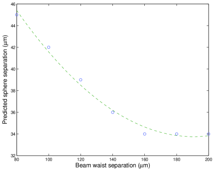
Figure 1: Sphere separation as a function of beam waist separation for 2 two 2.3$\mu m$ spheres. The rate of change of sphere separation is seen to drop off as the waist separation increases. The fit to a parabola is to aid the eye, rather than to suggest a quantitative relationship.

III.1 2.3 micron micrometer diameter spheres

We consider the case for chains of both two and three spheres. For two spheres we measure a sphere separation of  34$\mu m$, for a beam waist, $\omega_{0}=4.3\mu m$ at a laser wavelength, $\lambda=1064nm$. Using a beam waist separation of $180\mu m$ our model predicts an equilibrium in the scattering force of 34$\mu m$, as is shown in figure 2. The intensity in the x-z plane for this configuration is shown in figure 3. We see no such equilibrium in the gradient force, shown in figure 4 and conclude that the scattering force is the dominant factor in this instance. Using the same parameters for the three sphere case give us a sphere separation prediction of  62$\mu m$, as shown in figure 5. Again this dominates over the gradient force, this assumption being valid, as the theory gives a good prediction of our experimental observations. Our experimental result is 57$\mu m$, but we estimate our model value falls within the standard deviation error we observe on our experimental measurements.

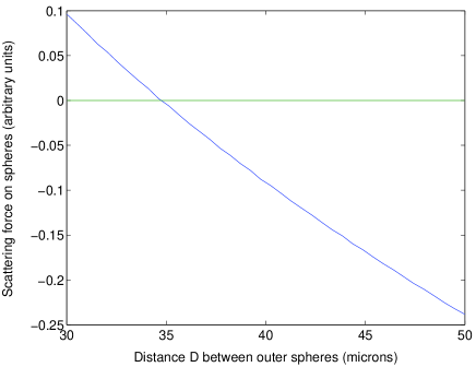
Figure 2: Scattering force on two 2.3 micron $\mu m$ diameter silica spheres with the beam waists 180 $\mu m$ apart. $\omega_{0}=3.5\mu m$ and $\lambda=1064nm$.

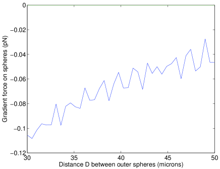
Figure 3: Gradient force on two 2.3 $\mu m$ diameter silica spheres with the beam waists 180 $\mu m$ apart. $\omega_{0}=3.5\mu m$ and $\lambda=1064nm$.

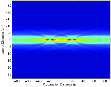
Figure 4: Intensity plot in the x-z plane for the case of two 2.3 $\mu m$ diameter silica spheres with the beam waists 180 $\mu m$ apart. $\omega_{0}=3.5\mu m$ and $\lambda=1064nm$.

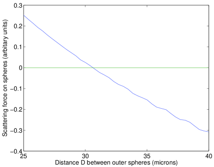
Figure 5: Scattering force on three 2.3 $\mu m$ diameter silica spheres with the beam waists 180 $\mu m$ apart. $\omega_{0}=3.5\mu m$ and $\lambda=1064nm$. The plot shows the separation between two of the three spheres, and the scattering forces are symmetric about the center sphere.

III.2 3 micrometer diameter spheres

The data for 3 micron spheres carried out at a different wavelength than the 2.3 $\mu m$ data ($\lambda=780nm$) also fits well with our theory. For two spheres, with the beam waists $150\mu m$ apart, we predict a sphere separation of  47$\mu m$ (figure 6) while our experiment predicts a distance of  45$\mu m$. Using the same parameters for the three sphere case we predict a sphere separation of 27$\mu m$ (figure 7), while our experiment shows a separation of  35$\mu m$. Again, as we predict equilibrium positions with the scattering force component, but not with the gradient force component, we conclude that the scattering force is the dominant factor in determining the final sphere separations.

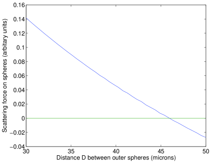
Figure 6: Scattering force on two 3 $\mu m$ diameter silica spheres with the beam waists 150 $\mu m$ apart. $\omega_{0}=4.3\mu m$ and $\lambda=780nm$.

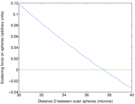
Figure 7: Scattering force on three 3 $\mu m$ diameter silica spheres with the beam waists 150 $\mu m$ apart. $\omega_{0}=4.3\mu m$ and $\lambda=780nm$. The plot shows the separation between two of the three spheres, and the scattering forces are symmetric about the center sphere.

IV Discussion and Conclusions

Our model accurately predicts separations for the case of two and three spheres, at certain sizes. However we also performed experiments using $1\mu m$ diameter spheres and could not find any agreement between experiment and theory. Since our model uses a paraxial approximation, the assumption is that in these smaller size regimes the model breaks down. This in contrast to the work detailed in Singer which works in size regimes closer to the laser wavelength, $\lambda$, and begins to break down in the larger size regimes ($\lambda>2l$), where $l$ is the sphere diameter.

We also note that the beam separation distance becomes less critical as it becomes larger. For small beam waist separation distances ($l<<80\mu m$, say), any change in this parameter leads to a sharp change in the sphere separation distance, whereas at the waist separation distances we work at the change in sphere separation distance is far more gentle, and hence gives less rise to uncertainty over exact fits with theory and experiment. The other main parameter is sphere size, which has an appreciable effect on the predicted sphere separation. The incident power on the spheres does not make much of a difference and is more of a scaling factor in the forces involved rather than a direct modifier in the model. Predicted sphere separation is also sensitive to the refractive index difference between the spheres and the surrounding medium, so it is important that the spheres’ refractive index is well known.

It should also be possible to create two-dimensional and possibly three dimensional arrays from optically bound matter. The extension to two dimensions is relatively simple to envisage with the use of multiple pairs of counterpropagating laser beams. In three dimensions the formation of such optically bound arrays may circumvent some of the problems associated with loading of three-dimensional optical lattices vanB . It is often assumed that the creation of an optical lattice (via multibeam interference, say) will allow the simple, unambiguous trapping of particles in all the lattice sites, thereby making an extended three-dimensional array of particles. Such arrays may be useful for crystal template formation vanB and in studies of crystallization processes Bechinger ; Reichhardt . However crystal formation in this manner is not particularly robust in that as the array is filled the particles perturb the propagating light field such that they prevent the trap sites below them being efficiently filled. Arrays of optically bound matter do not suffer from such problems, as they are organized as a result of the perturbation of the propagating fields. Further the fact that the particles are bound together provides more realistic opportunities for studying crystal and colloidal behaviour than that in unbound optically generated arrays, such as those produced holographically Grier1 ; Grier2 ; Bechinger .

We have developed a model by which the propagation of counter-propagating lasers beams moving past an array of silica spheres may be examined. Analysis of the resulting forces on the spheres allows us to predict the separation of the spheres which constitute the array. We have compared this model with experimental results for different beam parameters (wavelength, waist separation, waist diameter) and found the results to be in good agreement with our observations. The model, does not however, work with sphere sizes much less than approximately twice the laser wavelength. Our model is readily extendable to larger number of spheres, and will be of great use in the study of such one- and higher-dimensional arrays of optically bound matter.

References

- (1) Corresponding author. E-mail: dm11@st-and.ac.uk
- (2) A. Ashkin, Phys. Rev. Lett. 24 156 (1970).
- (3) A. Ashkin and J.M. Dziedzic, Appl. Phy. Lett. 19 283 (1971).
- (4) A. Ashkin and J.M. Dziedzic, Science 187 1073 (1975).
- (5) A. Ashkin, J.M. Dziedzic, J.E. Bjorkholm and S. Chu, Opt. Lett. 11, 288 (1986).
- (6) S. Chu, J.E. Bjorkholm, A. Ashkin and A. Cable, Phys. Rev. Lett. 57 314 (1986).
- (7) S.A. Tatarkova, A.E. Carruthers and K. Dholakia, Phys. Rev. Lett. 89 283901 (2002).
- (8) M. M. Burns, J.-M. Fournier, J. A. Golovchenko, Phys. Rev. Lett., 63, 1233 (1989)
- (9) M. M. Burns, J.-M. Fournier, J. A. Golovchenko, Science, 249, 749 (1990)
- (10) A. van Blaaderen, J.P. Hoogenboom, D.L.J. Vossen, A. Yethiraj, A. van der Horst, K. Visscher and M. Dogterom, Faraday Discuss. 123 107 (2003).
- (11) H.C. Nägerl, D. Leibfried, F. Schmidt-Kaler, J. Eschner, R. Blatt, Opt. Exp. 3, 89 (1998).
- (12) W. Singer, M. Frick, S. Bernet and M. Ritsch-Marte, J. Opt. Soc. Am. B 20 1568 (2003).
- (13) M.D. Feit and J.A. Fleck, Appl. Opt. 19 1154, (1980).
- (14) A. Rohrbach and E.H.K. Stelzer, Appl. Opt. bf 41, 2492 (2002).
- (15) M. Brunner and C. Bechinger, Phys. Rev. Lett. 88, 248302 (2002).
- (16) C. Reichhardt and C.J. Olson, Phys. Rev. Lett. 88 248301 (2002).
- (17) P. T. Korda, M. B. Taylor and D. G. Grier, Phys. Rev. Lett. 89, 128301 (2002).
- (18) P. T. Korda, G. C. Spalding, and D. G. Grier, Phys. Rev. B 66, 024504 (2002).