Optimal rotations of deformable bodies
and orbits in magnetic fields

Abstract

Deformations can induce rotation with zero angular momentum where dissipation is a natural “cost function”. This gives rise to an optimization problem of finding the most effective rotation with zero angular momentum. For certain plastic and viscous media in two dimensions the optimal path is the orbit of a charged particle on a surface of constant negative curvature with magnetic field whose total flux is half a quantum unit.

Rotations with zero angular momentum are intriguing. The most celebrated phenomenon of this kind is the rotation of a falling cat. A mechanical model ref:kane replacing the cat by two rigid bodies that can rotate relative to each other, has been extensively studied, see ref:montgomery ; ref:marsden and references therein. Here we address rotations with zero angular momentum under linear deformations. Our motivation comes from nano-mechanics: Imagine an elastic or plastic material with its own energy source, and ask what is the most efficient way of turning it through an appropriate sequence of autonomous deformations without external torque.

Deformations can generate rotations because order matters: A cycle of deformations will, in general, result in a rotation. The limiting ratio between the rotation and the area of the controls (deformations), when the latter tends to zero can be interpreted as curvature ref:novikov ; ref:shapere . Consequently, small cycles are ineffective since a cycle of length $\varepsilon$ in the controls leads to a rotation of order $\varepsilon^{2}$. The search for optimal paths forces one to mind deformations that are not small.

The problem we address has three parts. The first part is to determine the rotation for a given path of the controls. We solve this problem for general linear deformations. In two dimensions this leads to curvature on the space of the controls which is localized. If one thinks of the curvature as a magnetic field, then the total magnetic flux is half the quantum unit. The second part is to set up a model for the cost function which we choose to be a measure of dissipation. We focus on two settings, one where the dissipation is rate independent, as is the case in certain plastics, and the other where it is rate dependent as in liquids. Both cost functions lead to the same metric on the space of deformations. The third part is to pose and solve the problem of finding the path of minimal dissipation for a given rotation. In two dimensions and for either model of dissipation, the problem maps to finding the shortest path that starts at a given point and encloses a given amount magnetic flux. As we shall see, optimal paths tend to linger near the circle in the space of controls where the ratio of eigenvalues of the quadrupole moment of the body is $(\phi+\sqrt{\phi})^{2}$. $\phi=(1+\sqrt{5})/2$ is the golden ratio.

Deformations generate rotations because angular momentum is conserved ref:shapere . Consider a collection of point masses $m_{\alpha}$ at positions $x_{\alpha}$. Internal forces may deform the body, but there are no external forces. Suppose that the center of mass of the body is at rest at the origin and that the body has zero angular momentum. The total angular momentum, $L_{ij}$, must then stay zero for all times.

A linear deformation is represented by a matrix $M$ that sends $x\to Mx$. The $i,j$ component of the angular momentum is

$$L_{ij}=\mathrm{Tr}\,(\dot{M}QM^{t}\,\ell_{ij}),$$ (1)

where $Q$ is the quadrupole moment of the body

$$Q_{ij}=\sum_{\alpha}m_{\alpha}(x_{\alpha})_{i}(x_{\alpha})_{j}$$ (2)

and $\ell_{ij},\ i<j$ are the $n\choose 2$ generators of rotations in $n$ dimensions, i.e. $(x,\ell_{ij}y)=x_{i}y_{j}-x_{j}y_{i}$. Since $\ell_{ij}$ span the anti-symmetric matrices, the set of $n\choose 2$ equations $L_{ij}=0$ imply that the matrix $(dM)QM^{t}$ is symmetric.

Two immediate consequences of this symmetry are:

• Isotropic bodies: With $Q=1$, and $M$ close to the identity, the symmetry of $(dM)QM^{t}$ reduces to $dM$ being symmetric: the linear transformation must be a strain ref:landau .

• Pointers: Pointers are bodies with large aspect ratios, such as needles and discs. In the limit of infinite aspect ratio, $Q$ may be identified with a projection where $\dim Q$ is the dimension of the pointer. With $M$ near the identity, the symmetry of $(dM)Q$ implies that $(1-Q)(dM)Q=(1-Q)Q(dM)^{t}=0.$ Since $Q$ does not acquire a component in the normal direction, $1-Q$, under $dM$ a pointer keeps its orientation.

We now derive the fundamental relation between the response (rotation) and the controls (deformations). To this end we use the polar decomposition $M=RS$ with $R$ orthogonal and $S$ positive. Assuming $S$ positive is a choice of a gauge which makes the representation unique with $S=\sqrt{M^{t}M}$. The symmetry of $(dM)QM^{t}$ gives

$$\{\mathcal{A},SQS\}=SQ(dS)-(dS)QS,\quad\mathcal{A}=R^{-1}\kern-1.00006pt{\raise 3.44444pt\hbox{ -}}\kern-6.00006pt{d}R.$$ (3)

Eq. (3) determines the differential rotation, $\mathcal{A}$, in terms of the variation of the controls $dS$. The symbol $\kern-1.00006pt{\raise 3.44444pt\hbox{ -}}\kern-6.00006pt{d}$ stresses that the differential will not, in general, integrate to a function on the space of deformations. Geometrically, the differential rotation is the connection 1-form which fixes a notion of parallel transport.

Eq. (3) can be interpreted in terms of a variational principle: The motion is such that the kinetic energy is minimal for a given deformation. To see this, let $M=1$ and $\dot{M}=\dot{R}+\dot{S}$ with $\dot{R}$ antisymmetric (i.e. a rotation) and $\dot{S}$ symmetric (i.e. a strain). The kinetic energy is

$$E=\frac{1}{2}\mathrm{Tr}\,\big{(}\dot{M}Q\dot{M}^{t}\big{)}=\frac{1}{2}\,\mathrm{Tr}\,\big{(}(\dot{R}+\dot{S})Q(-\dot{R}+\dot{S})\big{)}\;.$$ (4)

Minimizing with respect to $\dot{R}$ gives

$$0=\delta E=\frac{1}{2}\mathrm{Tr}\,\big{(}\delta\dot{R}\big{(}-\{Q,\dot{R}\}+[Q,\dot{S}]\big{)}\;.$$ (5)

The trace is of a product of antisymmetric matrices, and its vanishing for an arbitrary antisymmetric $\delta\dot{R}$ implies $\{\dot{R},Q\}=[Q,\dot{S}]$ which is Eq. (3) for $M=1$.

One readily sees that if $\mathcal{A}$ is the solution of Eq. (3) given $S$ and $Q$, then it is also a solution for $\lambda S$ and $Q$ for $\lambda$ a scalar valued function. Hence scaling does not drive rotations and we may restrict ourselves to volume (or area) preserving deformations with $\det S=1$.

Since any $Q$ is obtainable by a linear deformation of the identity, we may assume without loss of generality that $Q=1$. Eq. (3) reduces to

$$\{\mathcal{A},S^{2}\}=[S,dS]\;.$$ (6)

Eq. (6) is conveniently solved in a basis where $S$ is diagonal. Let $s_{j}$ denote the eigenvalues of $S$ then

$$\mathcal{A}_{ij}=\frac{s_{i}-s_{j}}{s_{i}^{2}+s_{j}^{2}}\,(dS)_{ij}\;.$$ (7)

The curvature $F$ is more interesting than the connection. It is defined by $F=d\mathcal{A}+\mathcal{A}\wedge\mathcal{A}$. Calculation gives

$$F_{ij}=2\sum_{k}\frac{s_{i}\,s_{j}\,(s_{i}+s_{k})(s_{j}+s_{k})}{(s_{i}^{2}+s_{j}^{2})(s_{j}^{2}+s_{k}^{2})(s_{i}^{2}+s_{k}^{2})}\,(dS)_{ik}\wedge(dS)_{kj}\;.$$

The situation is particularly simple in two dimensions. We use the Pauli matrices $\sigma_{x},\sigma_{z},i\sigma_{y}$ and the identity as basis for the real $2\times 2$ matrices. The symmetric matrices make a three dimensional space that is conveniently parameterized by cylindrical coordinates:

$$S(t,\rho,\theta)=t+(\rho\cos\theta)\,\sigma_{x}+(\rho\sin\theta)\,\sigma_{z}\,\quad\rho\geq 0.$$ (8)

In this parametrization $\det S=t^{2}-\rho^{2}$ and positive matrices correspond to the cone $t>\rho$. Since $i\sigma_{y}$ is the generator of rotation in two dimensions ${\cal A}=-i\,\sigma_{y}\,\kern-1.00006pt{\raise 3.44444pt\hbox{ -}}\kern-6.00006pt{d}\varphi$. Eq. (6) can be readily solved for the connection $\kern-1.00006pt{\raise 3.44444pt\hbox{ -}}\kern-6.00006pt{d}\varphi$ whose differential is the curvature $F$. One finds

$$\kern-1.00006pt{\raise 3.44444pt\hbox{ -}}\kern-6.00006pt{d}\varphi=\frac{1}{1+\zeta^{2}}\,d\theta,\quad F=-\frac{1}{(1+\zeta^{2})^{2}}\,d(\zeta^{2})\wedge d\theta\,,$$ (9)

where $\zeta=t/\rho$. $F$ and $\kern-1.00006pt{\raise 3.44444pt\hbox{ -}}\kern-6.00006pt{d}\varphi$ are invariant under scaling of $S$, as they must be.

The total curvature associated with the area preserving deformations is then $\int_{t^{2}-\rho^{2}=1}F=\frac{1}{2}\int d\theta=\pi$. This implies that in any single closed cycle (i.e. one without self intersections), the angle of rotation is at most $\pi$. When interpreted as magnetic flux, $\pi$ corresponds to half a unit of quantum flux.

A geometric understanding of why the total curvature of orientation preserving deformations ($t>\rho$ in Eq. (8)) is $\pi$ comes from considering also the orientation reversing deformations ($t<\rho$ in Eq. (8)). When both are considered $\zeta$ takes values in $[0,\infty)$ and then $F$ coincides with the curvature of the canonical line bundle (Berry’s spin half) on the (stereographically projected) two sphere. The Chern number of the bundle is $1$ and the total curvature $2\pi$. The orientation preserving matrices correspond to the northern hemisphere, $\zeta>1$, and orientation reversing to the southern hemisphere, $\zeta<1$, rem:plane .

The cost function must include some measure of dissipation. For, without dissipation energy is a function of the controls and no change in energy is associated with a closed loop. We consider two models of dissipation in isotropic media. Both lead to the same metric on the space of controls, namely

$$(d\ell)^{2}=\,\mathrm{Tr}\left(S^{-2}\,d(S^{2})\otimes S^{-2}d(S^{2})\right)\ .$$ (10)

Consider a medium with viscosity tensor $\eta$. The power due to dissipation is

$$P=\frac{1}{2}\,\sum\eta^{ijkl}\dot{u}_{ij}\dot{u}_{kl}\;,$$ (11)

where $u$ is the strain tensor and $\dot{u}$ the strain rate. $S$ is related to $u$ by $2u=S^{2}-1$. To see this recall that the strain is defined as the change in the distance between two neighboring points caused by a deformation. If the deformation is described by a metric $g$ then $g=1+2u$, where $1$ is the metric associated with the undeformed reference system ref:landau . When considering linear deformation described by a symmetric matrix $S$, the resulting metric is $g=S^{2}$ (regarding the covariant components of $g$ as the elements of a positive matrix).

The space of (symmetric) 4-th rank isotropic tensors is two dimensional and spanned by the two viscosity coefficients $\eta$ and $\eta^{\prime}$ ref:landau

$$\eta^{ijkl}=\eta g^{ik}g^{jl}+\eta^{\prime}g^{ij}g^{kl}\ .$$ (12)

We therefore find that in an isotropic medium

$$P=2\eta\,Tr\left(g^{-1}\dot{g}g^{-1}\dot{g}\right)+2\eta^{\prime}\,Tr\,\left(g^{-1}\dot{g}\right)Tr\,\left(g^{-1}\dot{g}\right)$$ (13)

For volume preserving transformations the term multiplying $\eta^{\prime}$ vanishes and one is left with the first term alone. By choosing the unit of time appropriately one can take $\eta=1$. This leads to the metric of Eq. (10) which is invariant under congruence, $g\to AgA^{t}$, for an arbitrary invertible matrix $A$.

The dissipation in certain plastic materials can be rate independent. This is the continuum mechanics analog of the dissipation due to friction when one body slides on another ref:ori . In plastics, rate independence is a consequence of the Lévy-Mise constitutive relation: $s\,\delta\lambda=\delta u$, where $s$ is the stress and $\delta\lambda$ a scalar valued function ref:hill . The constitutive relation is formally the same as for fluids ref:hill , and by isotropy, the dissipation must be a function of $d\ell$ of Eq. (10). If the material is memoryless, dissipation is additive with respect to concatenating paths and must be proportional to $d\ell$.

Returning now to two dimensions, let us parameterize the area preserving transformation by: $(t,\rho,\theta)=(\cosh(\tau/2),\sinh(\tau/2),\theta)$. The metric Eq. (10) gives

$$(d\ell)^{2}=(d\tau)^{2}+\sinh^{2}\tau(d\theta)^{2}\,.$$ (14)

This metric gives the hyperboloid the geometry of the pseudo-sphere i.e. it makes it into a surface of constant negative curvature $-1$ ref:novikov . Geometrically, this corresponds to embedding the hyperboloid $t^{2}-\rho^{2}=1$ in Minkowski space.

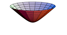
Figure 1: Positive, area preserving linear transformation may be identified with the hyperboloid of revolution $t^{2}-\rho^{2}=1$. Embedding the hyperboloid in Minkowski space gives it the structure of the Lobachevsky plane with constant negative curvature.

The metric enables us to assign a scalar $f$ to the curvature 2-form $F$ of Eq. (9) as the ratio between $F$ and the area form of the pseudo-sphere, $\sinh\tau\,d\tau\wedge d\theta$. Similarly, $a(\tau)$ is the scalar relating the length form $\sinh\tau\,d\theta$ to the one-form $\kern-1.00006pt{\raise 3.44444pt\hbox{ -}}\kern-6.00006pt{d}\varphi$. A calculation then gives

$$f(\tau)=\frac{1}{2\cosh^{2}\tau},\quad a(\tau)=\frac{\cosh\tau-1}{\sinh 2\tau}$$ (15)

and is plotted in Fig. 2. The curvature is everywhere positive and it is concentrated near the origin, $\tau=0$. It decays exponentially with $\tau$. This means that large deformations are ineffective. We already know that small deformations are ineffective. This brings us to the optimization problem.

Figure 2: The scalar curvature, $f(\tau)$, which can be interpreted as a magnetic field (left) and the $\theta$ component of the vector potential $a(\tau)$. $f$ is exponentially localized near the origin of the control space $(\tau,\theta)$, while $a$ has a maximum on the circle $\cosh\tau=\phi$, $\phi$ the golden ratio. $a^{2}/2$ appears also as a potential in the effective 1-dimensional dynamics of the optimization problem.

The control problem is to find a closed path $\gamma$ in the space of deformations, starting at $S_{0}=\sqrt{Q}_{0}$, ($Q_{0}$ is the initial quadrupole), which rotates the quadrupole by $\Phi$ radians, with minimal dissipation. If the dissipation is rate dependent, one adds a constraint that the time of traversal is $1$.

For viscous media $\gamma=\big{(}\tau(t),\theta(t)\big{)}$ is then the solution of the variational problem

$${\delta}\int_{0}^{1}\left(\frac{\dot{\tau}^{2}+\dot{\theta}^{2}\sinh^{2}\tau}{2}\,-\lambda a(\tau)\sinh(\tau)\dot{\theta}\right)dt=0$$ (16)

where $\lambda$ is a Lagrange multiplier and $\gamma(0)=\gamma(1)=S_{0}=S(\tau_{0},\theta_{0})$. This is the (variation of the) action of a classical particle with charge $\lambda$ and unit mass moving on the hyperbolic plane (i.e. the pseudo-sphere) in the presence of a magnetic field $f(\tau)$ given in Eq. (15).

Since motion in a magnetic field conserves kinetic energy the particle moves at constant speed and the dissipation, $\frac{1}{2}|\gamma|^{2}$, depends only on the length of the path. The variational problem can therefore be cast in purely geometric terms: Find the shortest closed path starting at a given point which encloses a given amount of magnetic flux. The shortest path is evidently also the solution in the case that the dissipation is rate independent.

Consider the family of isospectral deformations $\tau=const$ which keep the the eigenvalues of $S$ (or $Q$) constant while rotating its eigenvectors. We call these “stirring”, see Fig. 3. One can not stir an isotropic body, since its eigenvectors don’t have well defined directions.

Among the stirring cycles there is an optimal one which maximizes the rotation per unit length. From Eqs. (9,14) the flux to length ratio for stirring cycles is $a(\tau)$ of Eq. (9). The function $a$ takes its maximum at $\cosh\tau_{s}=\phi,\tau_{s}\approx 1.061$, see Fig. 2. Every cycle of the controls rotates by $\Phi_{s}=(2-\phi)\pi\approx.382\pi$ radians, somewhat less than a quarter turn.

To make full use of the optimal stirring cycle the initial conditions must be right. This is the case for a quadrupole with $Q=S(2\tau_{s},\theta)$, $\theta$ arbitrary. With other initial conditions and for large angles of rotations, the optimal paths approach the optimal stirring cycle, linger near it, eventually returning to the initial point. This is shown in Fig. 4 for a half turn of an isotropic body.

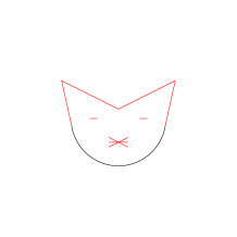
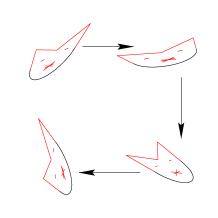
Figure 3: A reference shape (left), assumed to have $Q=1$, and four instances from the optimal stirring cycle (right). The configurations on the right are ordered clockwise with increasing $\theta$, starting with the top left. Both the first and the last correspond to $\theta=0$ and are therefore related by a pure rotation.

Figure 4: The optimal path in the space of shapes for a rotation by $\pi$ of a body with initial quadrupole moment $Q=1$. Polar coordinates $(\tau,\theta)$ are used to parametrize the plane. The path reaches exponentially close to the optimal stirring cycle at $\cosh\tau=\phi$, and winds around it twice before returning to the initial configuration. The optimal stirring cycle is not distinguishable from the envelope of the orbit in the scale of this figure.

Since the magnetic field $F(\tau)$ is rotationally invariant, the angular momentum

$$J=\sinh\tau\left(\dot{\theta}\sinh\tau-\lambda a(\tau)\right)$$ (17)

is conserved. Conservation of energy gives

$$0\leq\dot{\tau}^{2}=2E-\left(\frac{J}{\sinh\tau}+\lambda{a(\tau)}\right)^{2},$$ (18)

which reduces the problem to quadrature. The three conditions, $\tau(1)=\tau(0)$, $\theta(1)\equiv\theta(0)\,{\rm mod}\ 2\pi$, and the constraint of enclosed flux $\Phi$, determine the three parameters $E$, $J$ and $\lambda$.

The initial condition $\tau(0)=0$ is special: By Eq. (17) the angular momentum $J$ is forced to have the value 0. In turn, there is also one less condition to satisfy, as the value of $\theta$ when $\tau=0$ is meaningless. It then follows from Eqs. (17) and (18) that the optimal orbit, $\tau(\theta)$, depends only on the ratio $E/\lambda^{2}$. Rescaling time properly, we can achieve $\lambda=1$ by relaxing the constraint that the time to complete a cycle should be 1.

The key equation controlling the dynamics is Eq. (18), which describes effective one-dimensional motion in the potential $a^{2}(\tau)/2$. As shown above, $a(\tau)$ has a maximum at $\tau_{s}$. Therefore, closed orbits which correspond to optimal paths have energy values $E<a(\tau_{s})^{2}/2$. The motion is quite simple: Trajectories leave the origin with a positive $\dot{\tau}$, reach the turning point $\tau_{t}=a^{-1}(\sqrt{2E})$, and return symmetrically to the origin, thereby completing a cycle. The flux accumulated during a cycle is

$$\Phi=\int_{0}^{t_{\hbox{\tiny cycle}}}a(\tau)\sinh(\tau)\dot{\theta}dt\ ,$$ (19)

where $\dot{\theta}$ is obtained from Eq. (17).

Increasingly longer orbits are obtained when $E$ approaches the separatrix energy $a(\tau_{s})^{2}/2$. The orbit corresponding to the unstable equilibrium point at $\tau=\tau_{s}$ is the optimal stirring cycle, which is a $J=0$ orbit. The flux accumulated during a complete turn in parameter space, where $\theta$ increases by $2\pi$, is hence bounded by $\Phi_{s}$. Large values $\Phi$ require many turns during which the orbit approaches exponentially the optimal stirring cycle, see Fig. 4. A circular disc of playdough would therefore rotate by $\pi$, with no angular momentum, in about three cycles.

Acknowledgment: We thank Amos Ori for useful discussions. This work is supported by the Technion fund for promotion of research and by the EU grant HPRN-CT-2002-00277.

References

- (1) T.R. Kane and M.P.Scher, Int. J. Solid Structures 5, 663-670 (1969).
- (2) R. Montgomery, Fields Istitute Comm. 1, 193 (1993).
- (3) J. Marsden, Motion control and geometry, Proceeding of a Symposium, National Academy of Science 2003
- (4) B.A. Dubrovin, A.T. Fomenko, S.P. Novikov ; Modern geometry–methods and applications translated by Robert G. Burns, Springer (1992)
- (5) F. Wilczek and A. Shapere, Geometric Phases in Physics, World Scientific, Singapore, (1989).
- (6) Note that the plane represents the single matrix up to rotations and scaling.
- (7) L.D. Landau and I.M. Lifshitz, Theory of elasticity, Pergamon
- (8) R. Hill, The mathematical theory of plasticity, Oxford, (1950).
- (9) We are indebted to Amos Ori for this observation.