Ensembles of Protein Molecules as Statistical Analog Computers

Abstract

A class of analog computers built from large numbers of microscopic probabilistic machines is discussed. It is postulated that such computers are implemented in biological systems as ensembles of protein molecules. The formalism is based on an abstract computational model referred to as Protein Molecule Machine (PMM). A PMM is a continuous-time first-order Markov system with real input and output vectors, a finite set of discrete states, and the input-dependent conditional probability densities of state transitions. The output of a PMM is a function of its input and state. The components of input vector, called generalized potentials, can be interpreted as membrane potential, and concentrations of neurotransmitters. The components of output vector, called generalized currents, can represent ion currents, and the flows of second messengers. An Ensemble of PMMs (EPMM) is a set of independent identical PMMs with the same input vector, and the output vector equal to the sum of output vectors of individual PMMs. The paper suggests that biological neurons have much more sophisticated computational resources than the presently popular models of artificial neurons.

1 Introduction

After the classical work of Hodgkin and Huxley [6], it is widely recognized that the conformational changes in the sodium and potassium channels account for the generation of nerve spike. In this specific case, the time constants of the corresponding temporal processes are rather small (on the order of a few milliseconds). It is known that in some other cases (such as the ligand-gated channels) the time constants associated with conformational changes in protein molecules can have much larger values [1, 5, 9]. The growing body of evidence suggests that such slower conformational changes have direct behavioral implications [7, 8, 2]. That is, the dynamical computations performed by ensembles of protein molecules at the level of individual cells play important role in complex neuro-computing processes.

An attempt to formally connect some effects of cellular dynamics with statistical dynamics of conformations of membrane proteins was made in [4]. The present paper discusses a generalization of this formalism. The approach is based on an abstract computational model referred to as Protein Molecule Machine (PMM). The name expresses the hypothesis that such microscopic machines are implemented in biological neural networks as protein molecules. A PMM is a continuous-time first-order Markov system with real input and output vectors, a finite set of discrete states, and the input-dependent conditional probability densities of state transitions. The output of a PMM is a function of its input and state.

The components of input vector, called generalized potentials, can be interpreted as membrane potential, and concentrations of neurotransmitters. The components of output vector, called generalized currents, can be viewed as ion currents, and the flows of second messengers.

An Ensemble of PMMs (EPMM) is a set of independent identical PMMs with the same input vector, and the output vector equal to the sum of output vectors of individual PMMs. The paper explains how interacting EPMMs can work as robust statistical analog computers performing a variety of complex computations at the level of a single cell.

The EPMM formalism suggests that much more computational resources are available at the level of a single neuron than is postulated in traditional computational theories of neural networks. It was previously shown [2, 3] that such cellular computational resources are needed for the implementation of context-sensitive associative memories (CSAM) capable of producing various effects of working memory and temporal context.

A computer program employing the discussed formalism was developed. The program, called CHANNELS, allows the user to simulate the dynamics of a cell with up to ten different voltage-gated channels, each channel having up to eighteen states. Two simulation modes are supported: the Monte-Carlo mode (for the number of molecules from 1 to 10000), and the continuous mode (for the infinite number of molecules). New program capable of handling more complex types of PMMs is under development. (Visit the web site www.brain0.com for more information.)

The rest of the paper consists of the following sections:

1. Abstract Model of Protein Molecule Machine (PMM)

2. Example: Voltage-Gated Ion Channel as a PMM

3. Abstract Model of Ensemble of Protein Molecule Machines (EPMM)

4. EPMM as a Robust Analog Computer

5. Replacing Connections with Probabilities

6. Examples of Computer Simulation

7. EPMM as a Distributed State Machine (DSM)

8. Why Does the Brain Need Statistical Molecular Computations?

9. Summary

2 Abstract Model of Protein Molecule Machine (PMM)

A Protein Molecule Machine (PMM) is an abstract probabilistic computing system $(\textbf{X},\textbf{Y},\textbf{S},\alpha,\omega)$, where

• X and Y are the sets of real input and output vectors, respectively

• S$=\{s_{0},..s_{n-1}\}$ is a finite set of states

• $\alpha:\textbf{X}\times\textbf{S}\times\textbf{S}\to\textbf{R}^{\prime}$ is a function describing the input-dependent conditional probability densities of state transitions, where $\alpha(x,s_{i},s_{j})dt$ is the conditional probability of transfer from state $s_{j}$ to state $s_{i}$ during time interval $dt$, where $x\in\textbf{X}$ is the value of input, and $\textbf{R}^{\prime}$ is the set of non-negative real numbers. The components of $x$ are called generalized potentials. They can be interpreted as membrane potential, and concentrations of different neurotransmitters.

• $\omega:\textbf{X}\times\textbf{S}\rightarrow\textbf{Y}$ is a function describing output. The components of $y$ are called generalized currents. They can be interpreted as ion currents, and the flows of second messengers.

Let $x\in\textbf{X}$, $y\in\textbf{Y}$, $s\in\textbf{S}$ be, respectively, the values of input, output, and state at time t, and let $P_{i}$ be the probability that $s=s_{i}$. The work of a PMM is described as follows:

$$\frac{dP_{i}}{dt}=\sum_{j\neq i}{\alpha(x,s_{i},s_{j})P_{j}}-P_{i}\sum_{j\neq i}{\alpha(x,s_{j},s_{i})}$$ (1)

$$at\ t=0\qquad\sum_{i=0}^{n-1}{P_{i}}=1$$ (2)

$$y=\omega(x,s)$$ (3)

Summing the right and the left parts of (1) over $i=~{}0,..n-1$ yields

$$\frac{d(\sum_{i=0}^{n-1}{P_{i}})}{dt}=0$$ (4)

so the condition (2) holds for any t.

Figure 1: Internal structure of PMM

The internal structure of a PMM is shown in Figure 1, where $dp_{ij}$ is the probability of transition from state $s_{j}$ to state $s_{i}$ during time interval $dt$. The gray circle indicates the current state $s=s_{i}$. The output $y=~{}\omega(x,s)$ is a function of input and the current state.

For the probability of transition from state $s_{j}$ to state $s_{i}$ we have

$$dp_{ij}=\alpha(x,s_{i},s_{j})P_{j}dt$$ (5)

It follows from (1) that

$$dP_{i}=\sum_{j\neq i}{(dp_{ij}-dp_{ji})}$$ (6)

3 Example: Voltage-Gated Ion Channel as a PMM

Ion channels are studied by many different disciplines: biophysics, protein chemistry, molecular genetics, cell biology and others (see extensive bibliography in [5]).

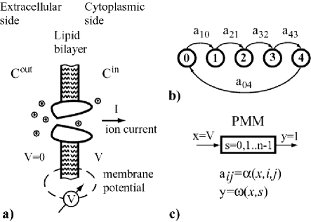
Figure 2: Ion channel as a PMM

This paper is concerned with the information processing (computational) possibilities of ion channels.

I postulate that, at the information processing level, ion channels (as well as some other membrane proteins) can be treated as PMMs. That is, at this level, the exact biophysical and biochemical mechanisms are not important. What is important are the properties of ion channels as abstract machines.

This situation can be meaningfully compared with the general relationship between statistical physics and thermodynamics. Only some properties of molecules of a gas (e.g., the number of degrees of freedom) are important at the level of thermodynamics. Similarly, only some properties of protein molecules are important at the level of statistical computations implemented by the ensembles of such molecules.

The general structure of a voltage-gated ion channel is shown schematically in Figure 2a. Figures 2b and 2c show how this channel can be represented as a PMM. In this example the PMM has five states $s\in\{0,1,..4\}$, a single input $x=V$ (the membrane potential) and a single output $y=I$ (the ion current). Using the Goldman-Hodgkin-Katz (GHK) current equation we have the following expression for the output function $\omega(x,s)$.

$$I_{j}=\omega(V,j)=\frac{p_{j}z^{2}FV^{\prime}(C^{in}-C^{out}e^{-zV^{\prime}})}{1-e^{-zV^{\prime}}}$$ (7)

where

• $I_{j}$ is the ion current in state $s=j$ with input $x=V$

• $p_{j}\ [cm/sec]$ is the permeability of the channel in state $s=j$

• $z$ is the valence of the ion ($z=1$ for $K^{+}$ and $Na^{+}$, $z=2$ for $Ca^{++}$)

• $F=9.6484\cdot 10^{4}\ [C/mol]$ is the Faraday constant

• $V^{\prime}=\frac{VF}{RT}$ is the ratio of membrane potential to the thermodynamic potential, where $T\ [K]$ is the absolute temperature, $R=8.3144\ [J/K\cdot~{}mol]$ is the gas constant

• $C^{in}$ and $C^{out}\ [mol]$ are the cytoplasmic and extracellular concentrations of the ion, respectively

One can make different assumptions about the function $\alpha(x,s_{j},s_{i})$, describing the conditional probability densities of state transitions. It is convenient to represent this function as a matrix of voltage dependent coefficients $a_{ij}(V)$.

$$\alpha=\begin{pmatrix}&a_{00}(V)\ ..\ a_{0j}(V)\ ..\ a_{0m}(V)\\ \\ &a_{i0}(V)\ ..\ a_{ij}(V)\ ..\ a_{im}(V)\\ \\ &a_{m0}(V)\ ..\ a_{mj}(V)\ ..\ a_{mm}(V)\end{pmatrix}$$ (8)

where $m=n-1$. Note that the diagonal elements of this matrix are not used in equation (1).

In the model of spike generation discussed in [4] both sodium, $Na^{+}$, and potassium, $K^{+}$ channels were treated as PMMs with five states shown in Figure 2. Coefficients $a_{10}$, $a_{21}$, $a_{32}$ where assumed to be sigmoid functions of membrane potential, and coefficients $a_{43}$ and $a_{04}$ - constant. In the case of the sodium channel, $s=3$ was used as a high permeability state, and $s=4$ was used as inactive state. In the case of potassium channel, $s=3$ and $s=4$ were assumed to be high permeability states.

Note. As the experiments with the program CHANNELS (mentioned in Section 1) show, in a model with two voltage-gated channels ($K^{+}$ and $Na^{+}$), the spike can be generated with many different assumptions about functions $\alpha$ and $\omega$.

4 Abstract Model of Ensemble of Protein Molecule Machines (EPMM)

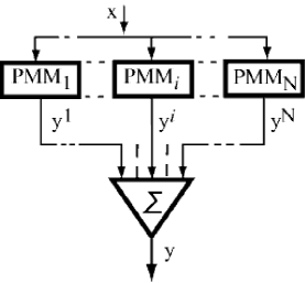
Figure 3: The structure of EPMM

An Ensemble of Protein Molecule Machines (EPMM) is a set of identical independent PMMs with the same input vector, and the output vector equal to the sum of output vectors of individual PMMs.

The structure of an EPMM is shown in Figure 3, where $N$ is the total number of PMMs, $y^{k}$ is the output vector of the k-th PMM, and $y$ is the output vector of the EPMM. We have

$$y=\sum_{k=1}^{N}y^{k}$$ (9)

Let $N_{i}$ denote the number of PMMs in state $s=i$ (the occupation number of state $i$). Instead of (9) we can write

$$y=\sum_{i=0}^{n-1}{N_{i}\omega(x,s_{i})}$$ (10)

$N_{i}$ $(i=0,...n-1)$ are random variables with the binomial probability distributions

$$P\{N_{i}=m\}=\binom{m}{N}P_{i}^{m}(1-P_{i})^{N-m}$$ (11)

$N_{i}$ has the mean $\mu_{i}=NP_{i}$ and the variance $\sigma_{i}^{2}=~{}NP_{i}(1-P_{i})$.

Let us define the relative number of PMMs in state $s=i$ (the relative occupation number of state $i$) as

$$e_{i}=\frac{N_{i}}{N}$$ (12)

The behavior of the average $\overline{e}_{i}$ is described by the equations similar to (1) and (2).

$$\frac{d\overline{e}_{i}}{dt}=\sum_{j\neq i}{\alpha(x,s_{i},s_{j})\overline{e}_{j}}-\overline{e}_{i}\sum_{j\neq i}{\alpha(x,s_{j},s_{i})}$$ (13)

$$at\ t=0\qquad\sum_{i=0}^{n-1}{\overline{e}_{i}}=1$$ (14)

The average output $\overline{y}$ is equal to the sum of average outputs for all states.

$$\overline{y}=N\sum_{i=0}^{n-1}{\omega(x,s_{i})\overline{e}_{i}}$$ (15)

The standard deviation for $e_{k}$ is equal to

$$\sigma_{k}=\sqrt{P_{k}(1-P_{k})/N}$$ (16)

It is convenient to think of the relative occupation numbers $e_{k}$ as the states of analog memory of an EPMM. In [2, 3, 4] the states of such dynamical cellular short-term memory (STM) were called E-states.

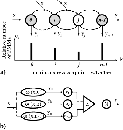
Figure 4: Relative occupation numbers of the microscopic states of a PMM as the macroscopic states of analog memory of the corresponding EPMM

Figure 4 illustrates the implementation of E-states as relative occupation numbers of the microscopic states of a PMM. The number of independent E-state variables is equal to $n-1$. The number is reduced by one because of the additional equation (14).

5 EPMM as a Robust Analog Computer

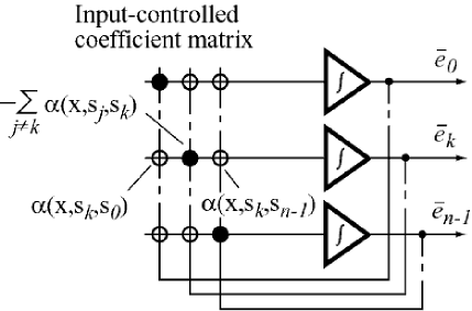
Figure 5: Simulation of an EPMM using integrating operational amplifiers with input–controlled coefficient matrix

An EPMM can serve as a robust analog computer with the input–controlled coefficient matrix shown in Figure 5. Since all the characteristics of the statistical implementation of this computer are determined by the properties of the underlying PMM, this statistical molecular implementation is very robust.

The implementation using $n$ integrating operational amplifiers shown in Figure 5 is not very reliable. The integrators based on operational amplifiers with negative capacitive feedback are not precise, so condition (14) will be gradually violated. (A better implementation should use any $n-1$ equations from (13) combined with equation $(\ref{eq15})$.) In the case of the discussed statistical implementation condition $(\ref{eq15})$ is guaranteed because the number of PMMs, $N$, is constant.

6 Replacing Connections with Probabilities

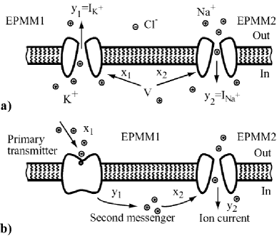
Figure 6: Two EPMMs interacting via a) electrical and b) chemical messages

The most remarkable property of the statistical implementation of the analog computer shown in Figure 5 is that the matrix of input-dependent macroscopic connections is implemented as the matrix of input-dependent microscopic probabilities. For a sufficiently large number of states (say, $n>10$), it would be practically impossible to implement the corresponding analog computers (with required biological dimensions) relying on traditional electronic operational amplifiers with negative capacitive feedbacks that would have to be connected via difficult to make matrices of input-dependent coefficients.

A single neuron can have many different EPMMs interacting via electrical messages (membrane potential) and chemical messages (different kinds of neurotransmitters). As mentioned in Section 3, the Hodgkin-Huxley [6] model can be naturally expressed in terms of two EPMMs (corresponding to the sodium and potassium channels) interacting via common membrane potential (see Figure 6a). Figure 6b shows two EPMMs interacting via a second messenger. In this example, EPMM1 is the primary transmitter receptor and EPMM2 is the second messenger receptor.

7 Examples of Computer Simulation

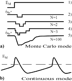
Figure 7: Examples of computer simulation by program CHANNELS

Figure 7 presents examples of computer simulation done by program CHANNELS mentioned in Section 1. Lines 2-4 in Figure 7a display random pulses of sodium current produced by 1, 2, and 3 PMMs, respectively, representing sodium channel, in response to the pulse of membrane potential shown in line 1. Line 4 shows a response of 100 PMMs. (A description of the corresponding patch-clamp experiments can be found in [11, 5]).

Figure 7b depicts the spike of membrane potential produced by two interacting EPMMs representing ensembles of sodium and potassium channels ($N\rightarrow\infty$).

In this simulation, the sodium and potassium channels were represented as five-state PMMs mentioned in Section 3. The specific values of parameters are not important for the purpose of this illustration.

8 EPMM as a Distributed State Machine (DSM)

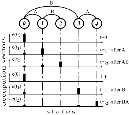
Figure 8: EPMM as a distributed state machine (DSM)

Let the number of PMMs go to infinity ($N\rightarrow\infty$). In this case EPMM is a deterministic system described by the set of differential equations 13 and 14. In some cases of highly nonlinear input-dependent coefficients $\alpha(x,i,j)$, it is convenient to think about this dynamical system as a distributed state machine (DSM). Such machine simultaneously occupies all its discrete states, with the levels of occupation described by the occupation vector $e=(e_{0},...e_{n-1})$. We replaced $\overline{e}_{i}$ by $e_{i}$, since $N\rightarrow\infty$.

This interpretation offers a convenient language for representing dynamical processes whose outcome depends on the sequence of input events. In the same way as a traditional state machine is used as a logic sequencer, a DSM can be used as an analog sequencer. The example shown in Figure 8 illustrates this interesting possibility.

If the sequence of input events is $AB$ the DSM ends up ”almost completely” in state 2 (lines 1-3). The BA sequence leads to state 4 (lines 4-6). Many different implementations of a DSM producing this sequencing effect can be found. Here is an example of an EPMM implementation:

Let $x=(x_{1},x_{2})$, $s\in\{0,1,2,3,4\}$, and let $\alpha(x,i,j)$ be described as follows: if input satisfies condition $x_{1}>x_{thr1}\ \&\ x_{2}\leq x_{thr2}$ (event A) then $\alpha(x,i,j)>0$ for transitions $(i,j)\in\{(1,0),(4,3)\}$; if input satisfies condition $x_{1}\leq x_{thr1}\ \&\ x_{2}>x_{thr2}$ (event B) then $\alpha(x,i,j)>0$ for transitions $(i,j)\in\{(2,1),(3,0)\}$. In all other cases $\alpha(x,i,j)=0$.

This example can be interpreted as follows. If input $x_{1}$ exceeds its threshold level $x_{thr1}$ before input $x_{2}$ exceeds its threshold level $x_{thr2}$, the EPMM ends up ”mostly” in state 2. If these events occur in the reverse direction, the EPMM ends up ”mostly” in state 4.

9 Why Does the Brain Need Statistical Molecular Computations?

Starting with the classical work of McCulloch and Pitts [10] it is well known that any computable function can be implemented as a network of rather simple artificial neurons. Though the original concept of the McCullough-Pitts logic neuron is now replaced by a more sophisticated model of a leaky integrate-and-fire (LIF) neuron [12], the latter model is still very simple as compared to the EPMM formalism discussed in the present paper.

Why does the brain need statistical molecular computations? Why is it not sufficient to do collective statistical computations at the level of neural networks? The answer to this question is straightforward. There is not enough neurons in the brain to implement the required computations – such as those associated with different effects of neuromodulation, working memory and temporal context [2, 3] – in the networks built from the traditional artificial neurons. (Visit www.brain0.com to find a discussion of this critically important issue.)

10 Summary

1. A class of statistical analog computers built from large numbers of microscopic probabilistic machines is introduced. The class is based on the abstract computational model called Protein Molecule Machine (PMM). The discussed statistical computers are represented as Ensembles of PMMs (EPMMs). (Sections 2 and 4.)

2. It is postulated that at the level of neural computations some protein molecules (e.g., ion channels) can be treated as PMMs. That is, at this level, specific biophysical and biochemical mechanisms are important only as tools for the physical implementation of PMMs with required abstract computational properties. (Section 3.)

3. The macroscopic states of analog memory of the discussed statistical computers are represented by the average relative occupation numbers of the microscopic states of PMMs. It was proposed [2, 3, 4] that such states of cellular analog memory are responsible for the psychological phenomena of working memory and temporal context (mental set). (Section 4.)

4. In some cases, it is useful to think of an EPMM as a distributed state machine (DSM) that simultaneously occupies all its discrete states with different levels of occupation. This approach offers a convenient language for representing dynamical processes whose outcome depends on the sequence of input events. (Section 8.)

5. A computer program employing the discussed formalism was developed. The program, called CHANNELS, allows the user to simulate the dynamics of a cell with up to ten different voltage-gated channels, each channel having up to eighteen states. Two simulation modes are supported: the Monte-Carlo mode (for the number of molecules from 1 to 10000), and the continuous mode (for the infinite number of molecules). New software capable of handling more complex types of PMMs is under development. (Visit the web site www.brain0.com for more information.)

Acknowledgements

I express my gratitude to Prof. B. Widrow, Prof. L. Stark, Prof. Y. Eliashberg, Prof. M. Gromov, Dr. I. Sobel, and Dr. P. Rovner for stimulating discussions. I am especially thankful to my wife A. Eliashberg for constant support and technical help.

References

- [1] Changeux, F. (1993). Chemical Signaling in the Brain. Scientific American, November, 58-62.
- [2] Eliashberg, V. (1989). Context-sensitive associative memory: ”Residual excitation” in neural networks as the mechanism of STM and mental set. Proceedings of IJCNN-89, June 18-22, 1989, Washington, D.C. vol. I, 67-75. Eliashberg, V. (1989).
- [3] Eliashberg, V. (1990). Universal learning neurocomputers. Proceeding of the Fourth Annual parallel processing symposium. California state university, Fullerton. April 4-6, 1990. 181-191.
- [4] Eliashberg, V. (1990). Molecular dynamics of short-term memory. Mathematical and Computer modeling in Science and Technology. vol. 14, 295-299.
- [5] Hille, B. (2001). Ion Channels of Excitable Membranes. Sinauer Associates. Sunderland, MA
- [6] Hodgkin, A.L., Huxley, A.F. 1952. A Quantitative Description of Membrane Current and its Application to Conduction and Excitation in Nerve. Journal of Physiology, 117, 500-544.
- [7] Kandel, E.R., and Spencer, W.A. (1968). Cellular Neurophysiological Approaches in the Study of Learning. Physiological Rev. 48, 65-134.
- [8] Kandel, E., Jessel,T., Schwartz, J. (2000). Principles of Neural Science. McGraw-Hill.
- [9] Marder, E., Thirumalai, V. (2002). Cellular, synaptic and network effects of neuromodulation. Neural Networks 15, 479-493 .
- [10] McCulloch, W. S. and Pitts, W. H. (1943). A logical calculus of the ideas immanent in nervous activity. Bulletin of Mathematical Biophysics, 5:115-133.
- [11] Nichols, J.G., Martin, A.R., Wallace B.G., (1992) From Neuron to Brain, Third Edition, Sinauer Associates.
- [12] Spiking Neurons in Neuroscience and Technology. 2001 Special Issue, Neural Networks Vol. 14.