Note on transformation to general curvilinear coordinates for Maxwell’s curl equations
(Is the magnetic field vector ‘axial’?)

Abstract

Arguments for $\mathbf{H}$ and $\mathbf{B}$ to be considered ‘axial’, or pseudo vectors, are revisited. As a point against, we examine the complex-coordinate method for numerical grid truncation and mode loss analysis proved very successful in computational electrodynamics. This method is not compatible with convention that $\mathbf{H}$ and $\mathbf{B}$ are axial.

1 Introduction

In physics, one often encounters ‘symmetries’, i.e. situations when structural fields (as the permittivity $\epsilon$ and permeability $\mu$ in classical macroscopic electrodynamics) are invariant under the given transformation $\mathbf{x}^{\prime}=\mathbf{x}^{\prime}(\mathbf{x})$. To obtain general conclusions on dynamic behavior of such symmetric systems without solving the governing dynamic equations, one needs to know also how the functional fields (electric and magnetic fields in Maxwell’s equations) are transformed with $\mathbf{x}^{\prime}=\mathbf{x}^{\prime}(\mathbf{x})$. Physical intuition and experiment is generally what provides us with this knowledge.

Important symmetries are with respect to coordinate reflections, as $\mathbf{x}\rightarrow\mathbf{x}^{\prime}=(-x^{1},x^{2},x^{3})$, and coordinate inversion, $\mathbf{x}\rightarrow\mathbf{x}^{\prime}=(-x^{1},-x^{2},-x^{3})=-\mathbf{x}$. These are improper transformations whose Jacobian, $J^{i^{\prime}}_{i}=\partial x^{i^{\prime}}/\partial x^{i}$, has negative determinant: $\det J^{i^{\prime}}_{i}=\Delta<0$. In numerous textbooks on classical mechanics and electrodynamics, vector-like objects are classified into polar, or ordinary vectors, and axial, or pseudo vectors — depending on their behavior under improper transformations. Polar vectors are transformed under inversion as $\mathbf{V}^{\prime}=-\mathbf{V}$, while axial as $\mathbf{W}^{\prime}=\mathbf{W}$.

The $\mathbf{V}^{\prime}=-\mathbf{V}$ transformation under coordinate inversion implies that the $\mathbf{V}$ vector remains unchanged in the reference (‘absolute’, ‘physical’) space. On the opposite, $\mathbf{W}$ is reflected in the absolute space upon coordinate inversion. How is it possible at all that such ‘unrealistic’ pseudo quantities, dependent on the way we describe them, survive in the physical picture of reality? The answer is that they are normally related to observable quantities through the cross product which is defined so that it compensates for the inversion of pseudo vectors in absolute space.

Such situation is not quite satisfactory, however. Although many quantities in classical physics are not directly observable (measurable) and hence their ‘realism’ can always be questioned by a radical empiricist, a natural trend is to put as much ‘realism’ into each quantity as possible. In this paper we discuss an alternative convention for the cross product that allows to eliminate pseudo quantities from classical physics. Interestingly, it turns out to be more than just a matter of convention or convenience once the complex-coordinate transformations are concerned.

2 Maxwell’s equations

Classical theory of electromagnetism is usually built upon the fundament of Maxwell’s equations — a set of dynamic field equations which we write in standard three-vector notation as

$$\nabla\widetilde{{}^{\times}}\mathbf{E} =-\dot{\widetilde{\mathbf{B}}},\qquad \nabla\cdot\widetilde{\mathbf{B}}=0,$$ (1)

$$\nabla\widetilde{{}^{\times}}\widetilde{\mathbf{H}} =\dot{\mathbf{D}}+\mathbf{j},\qquad \nabla\cdot\mathbf{D}=\rho,$$ (2)

accompanied, in the simplest case, by the constitutive relations $\mathbf{D}=\epsilon\mathbf{E}$ and $\widetilde{\mathbf{B}}=\mu\widetilde{\mathbf{H}}$. Dots over characters denote time derivatives; tildes over $\mathbf{H}$ and $\mathbf{B}$ show explicitly that these quantities are regarded as pseudo vectors (such notation follows J. A. Schouten [1]); curls $(\nabla\widetilde{{}^{\times}})^{ik}=\widetilde{\mathfrak{E}}^{ijk}\partial_{j}$ are also defined through the pseudo density $\widetilde{\mathfrak{E}}^{ijk}$, $i,j,k=1,2,3$, equal to the Levi-Civita permutation symbol $\varepsilon^{ijk}$ in any coordinate system [2, p. 158]:

$$\widetilde{\mathfrak{E}}^{i^{\prime}j^{\prime}k^{\prime}}=\Delta^{-1}J_{i}^{i^{\prime}}J_{j}^{j^{\prime}}J_{k}^{k^{\prime}}\widetilde{\mathfrak{E}}^{ijk},\qquad\widetilde{\mathfrak{E}}^{ijk}\doteq\varepsilon^{ijk}.$$ (3)

The $\doteq$ sign means equality in a given (here, in an arbitrary right- or left-hand) coordinate system. With use of classic ‘kernel-index’ notation, we write Maxwell’s equations (1), (2) in a more general form, valid assumably in arbitrary curvilinear, nonorthogonal coordinates:

$$\widetilde{\mathfrak{E}}^{ijk}\partial_{j}E_{k} =-\dot{\widetilde{\mathfrak{B}}}{}^{i},\qquad \partial_{i}\widetilde{\mathfrak{B}}^{i}=0,$$ (4)

$$\widetilde{\mathfrak{E}}^{ijk}\partial_{j}\widetilde{H}_{k} =\dot{\mathfrak{D}}^{i}+\mathfrak{j}^{i},\qquad \partial_{i}\mathfrak{D}^{i}=\rho.$$ (5)

Here $E_{i}$ and $\widetilde{H}_{i}$ are the covariant vector and pseudo vector; $\mathfrak{D}^{i}$ and $\widetilde{\mathfrak{B}}^{i}$ the contravariant vector density and pseudo density of weight $+1$, as reflected by Gothic kernels; $\mathfrak{j}^{i}$ and $\rho$ the contravariant vector and scalar densities. This form follows from the (here unquestioned) three-dimensional, generally covariant Maxwell’s equations [1, 3]

$$2\partial_{[i}E_{j]} =-\dot{B}_{ij},\qquad\partial_{[i}B_{jk]} =0,$$ (6)

$$\partial_{j}\mathfrak{H}^{ij} =\dot{\mathfrak{D}}^{i}+\mathfrak{j}^{i},\qquad\partial_{i}\mathfrak{D}^{i} =\rho,$$ (7)

if one makes use of the dual equivalents $\widetilde{\mathfrak{B}}^{i}=\frac{1}{2}\widetilde{\mathfrak{E}}^{ijk}B_{jk}$ and $\widetilde{H}_{i}=\frac{1}{2}\widetilde{\mathfrak{e}}_{ijk}\mathfrak{H}^{jk}$, as suggested e.g. by equations (2.35) and (2.37) in [3]. In (6) and (7), the square brackets denote alternation, $B_{ij}=-B_{ji}$ is the covariant bivector, and $\mathfrak{H}^{ij}=-\mathfrak{H}^{ji}$ the contravariant bivector density. Assuming the constitutive relations are $\widetilde{\mathfrak{B}}^{i}=\mu^{ij}\widetilde{H}_{j}$ and $\mathfrak{D}^{i}=\epsilon^{ij}E_{j}$, one concludes that the permittivity and permeability are tensor densities of weight $+1$, so that they are transformed as

$$\epsilon^{i^{\prime}j^{\prime}}=|\Delta|^{-1}J_{i}^{i^{\prime}}J_{j}^{j^{\prime}}\epsilon^{ij},\qquad\mu^{i^{\prime}j^{\prime}}=|\Delta|^{-1}J_{i}^{i^{\prime}}J_{j}^{j^{\prime}}\mu^{ij}.$$ (8)

An evident alternative to (4), (5) can be constructed by using in (6) and (7) the duals $\mathfrak{B}^{i}=\frac{1}{2}\mathfrak{E}^{ijk}B_{jk}$ and $H_{i}=\frac{1}{2}\mathfrak{e}_{ijk}\mathfrak{H}^{jk}$ instead, with the ordinary densities $\mathfrak{E}^{ijk}$ and $\mathfrak{e}_{ijk}$ equal to the Levi-Civita symbol for proper transformations, and changing the sign for improper ones:

$$\mathfrak{E}^{i^{\prime}j^{\prime}k^{\prime}}=|\Delta|^{-1}J_{i}^{i^{\prime}}J_{j}^{j^{\prime}}J_{k}^{k^{\prime}}\mathfrak{E}^{ijk},\qquad\mathfrak{E}^{ijk}\doteq\varepsilon^{ijk}.$$ (9)

Here $\doteq$ stands for equality in an arbitrary but right-hand coordinate system. We see no reason to agree that the duals constructed with $\mathfrak{E}^{ijk}$ and $\mathfrak{e}_{ijk}$ “are only meaningful for proper transformations” [3, p. 41]. An appropriate form of the generally covariant Maxwell’s equations — compare to (4), (5) — reads

$$\mathfrak{E}^{ijk}\partial_{j}E_{k} =-\dot{\mathfrak{B}}^{i},\qquad \partial_{i}\mathfrak{B}^{i}=0,$$ (10)

$$\mathfrak{E}^{ijk}\partial_{j}H_{k} =\dot{\mathfrak{D}}^{i}+\mathfrak{j}^{i},\qquad \partial_{i}\mathfrak{D}^{i}=\rho.$$ (11)

Given the constitutive relations are $\mathfrak{B}^{i}=\mu^{ij}H_{j}$ and $\mathfrak{D}^{i}=\epsilon^{ij}E_{j}$, the transformation laws for the permittivity and permeability are exactly the same as given by (8). In standard three-vector form, (10), (11) are reduced to the commonly known equations (1), (2) except for the tildes:

$$\nabla\times\mathbf{E} =-\dot{\mathbf{B}},\qquad \nabla\cdot\mathbf{B}=0,$$ (12)

$$\nabla\times\mathbf{H} =\dot{\mathbf{D}}+\mathbf{j},\qquad \nabla\cdot\mathbf{D}=\rho.$$ (13)

Two differences from the standard formulation thus is that all vectors are ‘polar’, and the curl $\nabla\times\mathbf{F}=\mathfrak{E}^{ijk}\partial_{j}F_{k}$. This seems perfectly sound were we to assign any ‘rigidity’ to the picture of magnetic ‘field lines’ for stationary media, instead of absolutizing the cross product definition by use of pseudo permutation objects.

3 Equivalence in real space

Most often in formulas that define observable (directly measurable) quantities in terms of $\mathbf{H}$ or $\mathbf{B}$, these latter fields enter in some conjunction with the vectorial product operation — like $\nabla\times\mathbf{H}$ in Ampere’s law, $\mathbf{j}\times\mathbf{B}$ in the expression for the Lorentz force density, or $\mathbf{H}^{\times}$ in the terms in constitutive relations accounting for induced optical activity. If we note that the neighboring tildes, if present, one over cross product and other over the $\mathbf{H}$ or $\mathbf{B}$ vector, do always annihilate, we conclude that the ‘polar-axial’ and ‘pure polar’ formulations of electrodynamics are largely equivalent.

Now we also show the equivalence of the two formulations in classifying the eigenmodes of symmetric systems by symmetry arguments. In the following, consider reflection with respect to the $x^{1}=0$ surface, $x^{1^{\prime}}=-x^{1}$. The corresponding Jacobian is $J^{i^{\prime}}_{i}=\mathrm{diag}(-1,1,1)=J^{i}_{i^{\prime}}$, its determinant $\Delta=-1$. It is well known that reflection symmetry of the system, $\epsilon^{\prime}(\mathbf{x}^{\prime})=\epsilon(\mathbf{x})$ and $\mu^{\prime}(\mathbf{x}^{\prime})=\mu(\mathbf{x})$, allows to replace the whole system by its half, with the PEC (the ‘electric wall’) or PMC (the ‘magnetic wall’) boundary standing in place of the reflection symmetry plane.

We write (10), (11) in terms of covariant electric and magnetic vectors:

$$\mathfrak{E}^{ijk}\partial_{j}E_{k} =-\mu^{ij}\dot{H}_{j},\qquad \partial_{i}\mu^{ij}H_{j}=0,$$ (14)

$$\mathfrak{E}^{ijk}\partial_{j}H_{k} =\epsilon^{ij}\dot{E}_{j}+\mathfrak{j}^{i},\qquad \partial_{i}\epsilon^{ij}E_{j}=\rho.$$ (15)

In the ‘pure polar’ formalism, both vectors are transformed under reflection as

$$E_{i^{\prime}}(\mathbf{x}^{\prime}) =J^{i}_{i^{\prime}}E_{i}(J^{i^{\prime}}_{i}x^{i})$$ (16)

$$=\{-E_{1}(-x^{1},x^{2},x^{3}),E_{2}(-x^{1},x^{2},x^{3}),E_{3}(-x^{1},x^{2},x^{3})\},$$

$$H_{i^{\prime}}(\mathbf{x}^{\prime}) =J^{i}_{i^{\prime}}H_{i}(J^{i^{\prime}}_{i}x^{i})$$ (17)

$$=\{-H_{1}(-x^{1},x^{2},x^{3}),H_{2}(-x^{1},x^{2},x^{3}),H_{3}(-x^{1},x^{2},x^{3})\}.$$

At the same time, if material objects are invariant under the given transform, so that $\epsilon^{i^{\prime}j^{\prime}}(\mathbf{x}^{\prime})=\epsilon^{ij}(\mathbf{x})$ and $\mu^{i^{\prime}j^{\prime}}(\mathbf{x}^{\prime})=\mu^{ij}(\mathbf{x})$, then Maxwell’s equations (14) and (15) remain unchanged except for the $-1$ multipliers acquired by the left-hand sides, owing to the transformation rule for $\mathfrak{E}^{ijk}$ (9). Thus the admissible new solutions (in the absence of free charges) are $E_{i^{\prime}}(\mathbf{x}^{\prime})=\pm\alpha E_{i}(\mathbf{x})$ and $H_{i^{\prime}}(\mathbf{x}^{\prime})=\mp\alpha H_{i}(\mathbf{x})$. Invariance of the physical system (material objects plus electromagnetic fields) to double reflection gives $\alpha^{2}=1$. Equating (16) with $E_{i}$ and (17) with $-H_{i}$ yields

$$\quad- E_{1}(-x^{1},x^{2},x^{3})=E_{1}(x^{1},x^{2},x^{3}),\quad- H_{1}(-x^{1},x^{2},x^{3})=-H_{1}(x^{1},x^{2},x^{3}),$$ (18a)

$$E_{2}(-x^{1},x^{2},x^{3})=E_{2}(x^{1},x^{2},x^{3}),\quad H_{2}(-x^{1},x^{2},x^{3})=-H_{2}(x^{1},x^{2},x^{3}),$$ (18b)

$$E_{3}(-x^{1},x^{2},x^{3})=E_{3}(x^{1},x^{2},x^{3}),\quad H_{3}(-x^{1},x^{2},x^{3})=-H_{3}(x^{1},x^{2},x^{3}).$$ (18c)

These conditions define even modes with the ‘numerical’ PMC plane at $x^{1}=0$: $E_{1}|_{x^{1}=0}=0$, $H_{2}|_{x^{1}=0}=0$, $H_{3}|_{x^{1}=0}=0$ (the ‘physical’ perfect conductor planes are not so readily expressed in nonorthogonal coordinates). The conditions obtained in a similar way with $\alpha=-1$ define the numerical PEC boundary and odd modes. Thus, the ‘pure polar’ Maxwell’s equations (10), (11) lead to exactly the same mode classification in optical waveguides and resonators exhibiting reflection symmetry as does the standard ‘polar-axial’ formulation.

4 Complex-coordinate scaling

In computational electrodynamics, the dominating way for treating unbounded problems in the finite-difference time-domain (FDTD), finite-difference frequency-domain, or finite-element calculations is with the perfectly matched layer (PML) method. Introduced originally in the ‘split-field’ formulation by J. P. Bérenger [4] and soon afterwards recast in the ‘uniaxial’ [5, 6] and stretched-coordinate [7, 8, 9, 10, 11] forms, the PML concept stands as “one of the most significant advances in the historical development of the FDTD method” [12].

The method is closely related to complex-coordinate transforms in classical quantum theory of atomic resonances [13] — though this is rarely appreciated by the electromagnetics modelling community. In electromagnetics, the method is implemented with surprising ease. Without loss of generality, we consider domain truncation in one, $x^{1}\equiv x$, direction. For media described by diagonal $\epsilon$ and $\mu$ matrices in the given coordinates, those matrices are modified in the PML regions according to

$$\hat{\epsilon}=\epsilon\mathrel{\mathop{\Lambda}\limits_{\mathop{x}}},\qquad\hat{\mu}=\mu\mathrel{\mathop{\Lambda}\limits_{\mathop{x}}},\qquad\mathrel{\mathop{\Lambda}\limits_{\mathop{x}}}\,=\left(\begin{array}[]{ccc}1/s_{x}&0&0\\ 0&s_{x}&0\\ 0&0&s_{x}\\ \end{array}\right)$$ (18s)

with the complex function

$$s_{x}(x^{\prime},\omega)=\zeta(x^{\prime})+\mathrm{i}\frac{\sigma(x^{\prime})}{\omega}$$ (18t)

where $x^{\prime}\in[-b,b]$ is the bounded computation-space coordinate, $\zeta(x^{\prime})$ and $\sigma(x^{\prime})$ are real-valued functions equal to 1 and, respectively, 0 over $[-a,a]\subset[-b,b]$, while $\sigma(x^{\prime})>0$ for $a<|x^{\prime}|\leq b$ in order to damp the $\exp[\mathrm{i}(kx^{\prime}-\omega t)]$ oscillatory waves inside the PML regions. Odd-power frequency dependence is included in the imaginary part of (18t), and hence in (18s), for causality reasons [14, §123]. It is repeatedly claimed that the structure of permittivity and permeability modified within the PMLs according to (18s) can be recovered by complex coordinate scaling

$$x=\int_{0}^{x^{\prime}}s_{x}(x^{\prime},\omega)\,\mathrm{d}x^{\prime}.$$ (18u)

It is easy to see however, that only the ‘pure polar’ formulation (10), (11) leads to (18s). In contrast, (4) and (5) yield

$$\mathrel{\mathop{\Lambda}\limits_{\mathop{x}}}\,=\left(\begin{array}[]{ccc}|s_{x}|/s_{x}^{2}&0&0\\ 0&|s_{x}|&0\\ 0&0&|s_{x}|\\ \end{array}\right)$$ (18v)

which is reduced to (18s) for real-valued coordinate squeezing [15], but essentially differs from (18s) given the $s_{x}$ function complex.

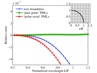
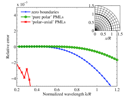
Figure 1: Mode index errors on Cartesian (left) and polar (right) grids. The superiority of the standard perfectly matched layers compatible with the ‘pure polar’ Maxwell’s equations (10), (11) is evident.

In order to compare the performance of (18v) and (18s), we simulated the fundamental mode of a step-index fiber ($n_{\mathrm{core}}/n_{\mathrm{clad}}=1.515/1.5$ as in [15, 16]) with the two-dimensional finite-difference frequency-domain method on Cartesian and polar grids. In figure 1, the fundamental mode index errors are plotted, associated with the standard (‘pure polar’ consistent) PMLs, the ‘polar-axial’ PMLs, and simple zero boundaries. The corresponding physical domains are $[0\dots 1.5R]\times[0\dots 1.5R]$ and $[0\dots 1.5R]\times[0\dots\pi/2]$, with resolution $40\times 40$ and $40\times 20$ pixels, respectively.

5 Summary

Standard (‘polar-axial’) and alternative (‘pure polar’) formulations of Maxwell’s equations were presented in section 2. In most cases, as illustrated in section 3, both approaches yield equivalent description of electromagnetics phenomena. In section 4 we pointed however that it is the ‘pure polar’ formalism that complies with the PML method used with much success in computational electrodynamics. An interesting question is, To which extent can the classic electric and magnetic fields — whose parity is a matter of controversy — be associated with the ‘electric $2^{j}$-pole’ and ‘magnetic $2^{j}$-pole’ photon states of different parity in quantum electrodynamics?

References

References

- [1] Schouten J A 1951 Tensor Analysis for Physicists (Oxford: Clarendon)
- [2] Levi-Civita T 1927 The Absolute Differential Calculus (London: Blackie & Son)
- [3] Post E J 1962 Formal Structure of Electromagnetics (Amsterdam: North-Holland)
- [4] Bérenger J P 1994 J. Comput. Phys. 114 185–200
- [5] Sacks Z S, Kingsland D M, Lee R and Lee J F 1995 IEEE Trans. Antennas Prop. 43 1460–3
- [6] Gedney S D 1996 IEEE Trans. Antennas Prop. 44 1630–9
- [7] Chew W C and Weedon W H 1994 Microwave Opt. Tech. Lett. 7 599–604
- [8] Rappaport C M 1995 IEEE Microwave Guided Wave Lett. 5 90–2
- [9] Petropoulos P G 1998 Appl. Munerical Math. 33 517–24
- [10] Teixeira F L and Chew W C 1998 IEEE Microwave Guided Wave Lett. 8 223–5
- [11] Hugonin J P and Lalanne P 2005 J. Opt. Soc. Am. A 22 1844–9
- [12] Taflove A (ed) 1998 Advances in Computational Electrodynamics (Boston: Artech House) ch 5
- [13] Moiseyev N 1998 Phys. Rep. 302 211–93
- [14] Landau L D and Lifshitz E M 1976 Statistical Physics (Moscow: Naüka) part I
- [15] Shyroki D M 2006 IEEE Microwave Wireless Comp. Lett. 16 576–8
- [16] Tsuji Y and Koshiba M 2000 J. Lightwave Technol. 18 618–23