On the Capacity of Nonlinear Fiber Channels

Haiqing Wei^∗ and David V. Plant

Department of Electrical and Computer Engineering
McGill University, Montreal, Canada H3A-2A6

^∗hwei1@po-box.mcgill.ca

Abstract

The nonlinearity of a transmission fiber may be compensated by a specialty fiber and an optical phase conjugator. Such combination may be used to pre-distort signals before each fiber span so to linearize an entire transmission line.

© 2024 Optical Society of America
OCIS codes: (060.2330) Fiber optics communications; (190.4370) Nonlinear optics, fibers

A fiber-optic transmission line is a nonlinear channel due to the material nonlinear effects. Fiber nonlinearity has become one of the major limiting factors in modern optical transmission systems [1, 2]. Distributed Raman amplification and various return-to-zero (RZ) modulation formats may be employed to reduce the nonlinear impairments, but merely to a limited extent. It is known that the nonlinearity of one fiber line may be compensated by that of another with the help of optical phase conjugation (OPC). However, all previous proposals and demonstrations [3, 4, 5, 6, 7] work partially in fighting the fiber nonlinearity. They either are specialized to only one aspect of the nonlinear effects, or fail to work in the presence of dispersion slope or higher order dispersion effects. Still open to date is an important question: does fiber nonlinearity really impose a fundamental limit to the channel capacity? This paper introduces the notion of scaled nonlinearity, which together with the application of OPC, provides a negative answer to the above question.

Consider an optical fiber stretching from $z=-L$ to $z=0$, along which the optical birefringence is either vanishingly weak to avoid the effect of polarization mode dispersion (PMD), or sufficiently strong to render the fiber polarization maintaining. A set of optical signals are wavelength-division multiplexed (WDM) and injected into the fiber. For simplicity, it is assumed that all the signals are co-linearly polarized, and coupled into one polarization eigen state when the fiber is polarization maintaining. The signals may be represented by a sum of scalars $E({\bf r},t)=F(x,y)\sum_{n}A_{n}(z,t)\exp\left[i\int^{z}\beta(\zeta,\omega_{n})d\zeta-i\omega_{n}t\right]$, where $F(x,y)$ is the transverse modal function, $\forall n\in{\bf Z}$, $\omega_{n}=\omega_{0}+n\Delta$ and $A_{n}$ are the center frequency and the signal envelope of the $n$th WDM channel respectively, $\Delta>0$ is the channel spacing, $\beta(z,\omega)$ is the function of propagation constant vs. optical frequency $\omega$ at the position $z$ in the fiber. Define $\beta^{(k)}(z,\omega)\stackrel{{\scriptstyle\rm def}}{{=}}\frac{\partial^{k}}{\partial\omega^{k}}\beta(z,\omega)$, $\forall k>0$. The dynamics of signal propagation may be described by a group of coupled partial differential equations [8, 9],

$$\frac{\partial A_{n}}{\partial z}-i\beta_{1n}\left(z,i\frac{\partial}{\partial t}\right)A_{n}+\frac{\alpha_{n}(z)}{2}A_{n}=i\gamma(z)\sum_{k}\sum_{l}A_{k}A_{l}A_{k+l-n}^{*}\exp[i\theta_{kln}(z)]+\sum_{m}g_{mn}(z)|A_{m}|^{2}A_{n},$$ (1)

$\forall n\in{\bf Z}$, $-L\leq z\leq 0$, where $\gamma$ is the Kerr nonlinear coefficient, $\alpha_{n}$ is the attenuation coefficient around $\omega_{n}$, $g_{mn}$ is the Raman coupling coefficient from the $m$th to the $n$th channels, $\theta_{kln}(z)\stackrel{{\scriptstyle\rm def}}{{=}}\int^{z}[\beta(\zeta,\omega_{k})+\beta(\zeta,\omega_{l})-\beta(\zeta,\omega_{k+l-n})-\beta(\zeta,\omega_{n})]d\zeta$ denotes the phase mismatch among the mixing waves, and $\beta_{1n}$ is a functional operator defined as $\beta_{1n}(z,i\frac{\partial}{\partial t})\stackrel{{\scriptstyle\rm def}}{{=}}\sum_{k=1}^{+\infty}\frac{1}{k!}\beta^{(k)}(z,\omega_{n})\left(i\frac{\partial}{\partial t}\right)^{k}$. Using the frame transformation $(z,t)\rightarrow\left(z,t+\int^{z}\beta^{(1)}(\zeta,\omega_{0})d\zeta\right)$, (1) may be rewritten as,

$$\frac{\partial A_{n}}{\partial z}-i\beta_{2n}\left(z,i\frac{\partial}{\partial t}\right)A_{n}+\frac{\alpha_{n}(z)}{2}A_{n}=i\gamma(z)\sum_{k}\sum_{l}A_{k}A_{l}A_{k+l-n}^{*}\exp[i\theta_{kln}(z)]+\sum_{m}g_{mn}(z)|A_{m}|^{2}A_{n},$$ (2)

$\forall n\in{\bf Z}$, $-L\leq z\leq 0$, with $\beta_{2n}\left(z,i\frac{\partial}{\partial t}\right)\stackrel{{\scriptstyle\rm def}}{{=}}\beta_{1n}\left(z,i\frac{\partial}{\partial t}\right)-\beta^{(1)}(z,\omega_{0})\left(i\frac{\partial}{\partial t}\right)$. This set of equations completely determine the propagation dynamics of the optical signals. In case the signals are not co-linearly polarized, the mathematical description should be slightly modified to deal with the complication. However, the same physics remains to govern the nonlinear signal propagation in optical fibers, still valid are the method of nonlinearity compensation described below and the conclusion about the capacity of nonlinear channels.

When the signals become intense, the nonlinear interaction as evidenced in (2) can badly distort them and make the carried information difficult to retrieve. Unlike the case of linear channels [10], simply raising the signal power may not necessarily increase the capacity of a nonlinear channel. Nevertheless, the nonlinear interaction among the signals is deterministic in nature that can be undone in principle. The question is how to implement a physical device which undoes the distortion. Suppose there is a specialty fiber stretching from $z=0$ to $z=L/R$, $R>0$ being a constant, in which $q(z,\omega)$ is the optical propagation constant. Let a set of WDM signals $E^{\prime}({\bf r},t)=F^{\prime}(x,y)\sum_{n}A^{\prime}_{n}(z,t)\exp\left[i\int^{z}q(\zeta,\omega^{\prime}_{n})d\zeta-i\omega^{\prime}_{n}t\right]$ propagate in the specialty fiber, where $\forall n\in{\bf Z}$, $\omega^{\prime}_{n}=\omega^{\prime}_{0}+n\Delta$, $\omega^{\prime}_{0}$ may differ from $\omega_{0}$. As in the previous mathematical treatment, define a functional operator $q_{2n}(z,i\frac{\partial}{\partial t})\stackrel{{\scriptstyle\rm def}}{{=}}\sum_{k=1}^{+\infty}\frac{1}{k!}q^{(k)}(z,\omega^{\prime}_{n})\left(i\frac{\partial}{\partial t}\right)^{k}-q^{(1)}(z,\omega^{\prime}_{0})\left(i\frac{\partial}{\partial t}\right)$, with $q^{(k)}(z,\omega)\stackrel{{\scriptstyle\rm def}}{{=}}\frac{\partial^{k}}{\partial\omega^{k}}q(z,\omega)$, and let $\alpha^{\prime}_{n}$, $\gamma^{\prime}$, $\theta^{\prime}_{kln}$, $g^{\prime}_{mn}$ denote the linear and nonlinear parameters associated with the specialty fiber and the new set of WDM signals, then the propagation dynamics is governed by a similar group of equations,

$$\frac{\partial A^{\prime}_{n}}{\partial z}-iq_{2n}\left(z,i\frac{\partial}{\partial t}\right)A^{\prime}_{n}+\frac{\alpha^{\prime}_{n}(z)}{2}A^{\prime}_{n}=i\gamma^{\prime}(z)\sum_{k}\sum_{l}A^{\prime}_{k}A^{\prime}_{l}A^{\prime*}_{k+l-n}\exp[i\theta^{\prime}_{kln}(z)]+\sum_{m}g^{\prime}_{mn}(z)|A^{\prime}_{m}|^{2}A^{\prime}_{n},$$ (3)

$\forall n\in{\bf Z}$, $0\leq z\leq L/R$. If the parameters are set according to the following rules of scaling,

$$q^{(2)}(z,\omega^{\prime}_{0}+\omega) = R\beta^{(2)}(-Rz,\omega_{0}-\omega),~{}~{}\forall\omega\in{\bf R},$$ (4)

$$\alpha^{\prime}_{n}(z) = -R\alpha_{-n}(-Rz),~{}~{}\forall n\in{\bf Z},$$ (5)

$$\gamma^{\prime}(z) = R\gamma(-Rz)|C|^{-2},$$ (6)

$$g^{\prime}_{mn}(z) = -Rg_{-m,-n}(-Rz)|C|^{-2},~{}~{}\forall m,n\in{\bf Z},$$ (7)

$\forall z\in[0,L/R]$, $C\neq 0$ being a constant, then equations (3) are reduced from (2) by taking the complex conjugate, making a substitution $z\rightarrow-Rz$, and replacing $A^{*}_{-n}(-Rz,t)$ by $A^{\prime}_{n}(z,t)/C$. Mathematically, it says that $A^{\prime}_{n}(z,t)=CA^{*}_{-n}(-Rz,t)$, $\forall n\in{\bf Z}$, solve (3), which govern the nonlinear propagation in the specialty fiber. Interpreted physically, if OPC is applied after the transmission but before the specialty fibers to convert the signals $A_{n}(0,t)$, $n\in{\bf Z}$, into $A^{\prime}_{n}(0,t)=CA^{*}_{-n}(0,t)$, $n\in{\bf Z}$, then the specialty fiber will propagate the optical signals in a reversed manner with respect to the transmission fiber. At the end, the specialty fiber outputs signals $A^{\prime}_{n}(L/R,t)=CA^{*}_{-n}(-L,t)$, $n\in{\bf Z}$, which are replicas of the initial signals before entering the transmission fiber up to complex conjugation. The fibers and optical signals on the two sides are said to be mirror symmetric about the OPC, although in a scaled sense. Note that the specialty fiber would amplify light in correspondence to the attenuation in the transmission fiber and vice versa.

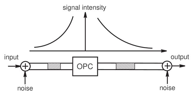
Fig. 1: A specialty fiber and a transmission fiber are in scaled mirror symmetry about the point of OPC. The shaded fiber segments are located at $-z$ and $Rz$ respectively, $0\leq z\leq L/R$, with the parameters $q^{(2)}(-z)$, $\alpha^{\prime}(-z)$, $\gamma^{\prime}(-z)$, $g^{\prime}(-z)$ proportional to $\beta^{(2)}(Rz)$, $\alpha(Rz)$, $\gamma(Rz)$, $g(Rz)$ as in (4-7).

So OPC and a specialty fiber with parameters designed according to (4-7) could perfectly compensate the nonlinearity of a transmission fiber, if not for the ever-existing noise, especially that incurred when the signal amplitude is low, destroying the mirror symmetry. A better designed link would start with a specialty fiber that boosts the power of the optical signals, followed by OPC, then a fiber for transmission in which the signal power decreases, as shown in Fig.1. In the fiber locations not too far from the OPC, the signal power is relatively high to minimize the effect of the optical noise, which usually originates from amplified spontaneous emission (ASE) and quantum photon statistics. However at the two ends of the link, the effect of the optical noise could become substantial. A simple but fairly accurate model may assume that optical noise is incurred exclusively at the two extreme ends of the link, dispersive and nonlinear signal propagation is the only effect of the inner part of the link. In this model, the nonlinearity of a segment of transmission fiber with $z_{1}\leq z\leq z_{2}$ is fully compensated by the portion of the specialty fiber with $-z_{2}/R\leq z\leq-z_{1}/R$, $\forall z_{1},z_{2}\in[0,L]$. In particular, the entire link from $z=-L/R$ to $z=L$ is equivalent to a linear channel impaired by additive noise at the two ends. If $W$ is the total optical bandwidth of the input WDM channels, then the OPC should have a bandwidth wider than $W$ to cover the extra frequency components generated through wave mixing in the specialty fiber. With nonzero dispersion fibers, however, the extra bandwidth due to wave mixing may hardly exceed $100$ GHz, which is often negligible in comparison to the total bandwidth $W$ of several, even tens of THz. Thus the linearized link may be assumed to have the same bandwidth limit $W$ throughout, applicable to which is Shannon’s formula for channel capacity [10], $C=W\log_{2}(1+S/N)$. Obviously, many of such linearized links may be cascaded to reach a longer transmission distance, and the entire transmission line is still linear end-to-end in spite of the nonlinearity existing locally in the fibers.

Using a commercial software, computer simulation has been carried out to test the proposed method of nonlinearity compensation. As in Fig.1, the simulated link consists of a specialty fiber, an OPC, and a transmission fiber that is of the negative nonzero dispersion-shifted type, $200$ km long, with loss coefficient $\alpha=0.2$ dB/km, dispersion $D=-8$ ps/nm/km, dispersion slope $S=0.08$ ps/nm²/km, effective mode area $A_{\rm eff}=50$ $\mu$m², Kerr and Raman coefficients that are typical of silica glass. The specialty fiber is a dispersion compensating fiber of the same material, but with parameters $(\alpha^{\prime},D^{\prime},S^{\prime})=20\times(-\alpha,D,-S)$ and $A^{\prime}_{\rm eff}=12.5$ $\mu$m². The nonlinearity of the specialty fiber can be switched on and off. ASE noise is added at the two ends of the link. The input consists of four WDM channels at $100$ GHz spacing, all RZ modulated at $10$ Gb/s with $33\%$ duty. The power of all optical pulses is peaked at $100$ mW when entering the transmission fiber. Fig.2 shows the received signals without and with nonlinearity in the specialty fiber respectively. Showing no nonlinear degradation, only the effect of ASE noise, the graph on the right side demonstrates clearly the compensation of optical nonlinearity.

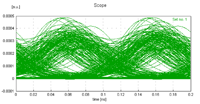
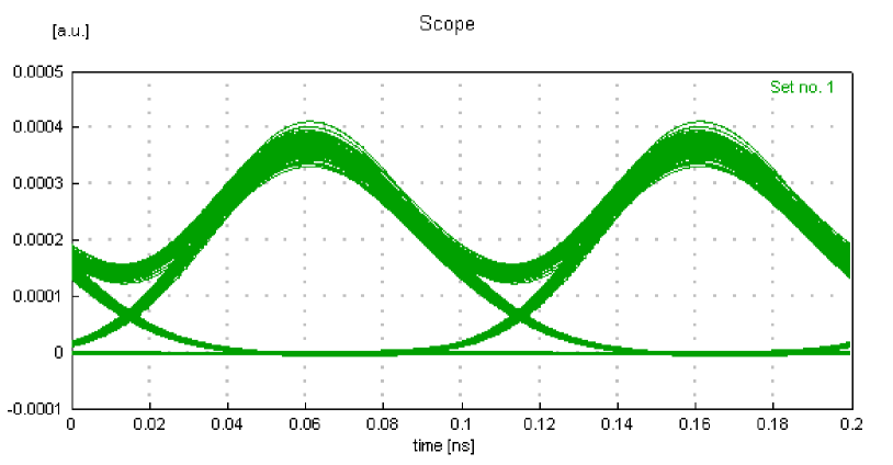
Fig. 2: Received signals at the end of a simulated link. Left: only the dispersion of the transmission fiber is pre-compensated by the specialty fiber. Right: both dispersion and nonlinearity are pre-compensated.

References

- [1] F. Forghieri, R. W. Tkach and A. R. Chraplyvy, “Fiber nonlinearities and their impact on transmission systems,” in Optical Fiber Telecommunications III A, I. P. Kaminow and T. L. Koch, eds. Academic Press: San Diego, 1997.
- [2] P. P. Mitra and J. B. Stark, “Nonlinear limits to the information capacity of optical fiber communications,” Nature, vol. 411, pp. 1027-1030, June 2001.
- [3] D. M. Pepper and A. Yariv, “Compensation for phase distortions in nonlinear media by phase conjugation,” Opt. Lett., vol. 5, pp. 59-60, 1980.
- [4] S. Watanabe, G. Ishikawa, T. Naito, and T. Chikama, “Generation of optical phase-conjugate waves and compensation for pulse shape distortion in a single-mode fiber,” J. Lightwave Technol., vol. 12, no. 12, pp. 2139-2146, 1994.
- [5] S. Watanabe and M. Shirasaki, “Exact compensation for both chromatic dispersion and Kerr effect in a transmission fiber using optical phase conjugation,” J. Lightwave Techn., vol. 14, no. 3, pp. 243-248, 1996.
- [6] A. G. Grandpierre, D. N. Christodoulides, and J. Toulouse, “Theory of stimulated Raman scattering cancellation in wavelength-division-multiplexed systems via spectral inversion,” IEEE Photon. Technol. Lett., vol. 11, no. 10, pp. 1271-1273, 1999.
- [7] I. Brener, B. Mikkelsen, K. Rottwitt, W. Burkett, G. Raybon, J. B. Stark, K. Parameswaran, M. H. Chou, M. M. Fejer, E. E. Chaban, R. Harel, D. L. Philen, and S. Kosinski, “Cancellation of all Kerr nonlinearities in long fiber spans using a LiNbO3 phase conjugator and Raman amplification,” OFC’00, post-deadline paper, PD33, Baltimore, Maryland, 2000.
- [8] Y. R. Shen, The Principles of Nonlinear Optics. New York: John Wiley & Sons, 1984.
- [9] G. P. Agrawal, Nonlinear Fiber Optics, 2nd ed. San Diego: Academic Press, 1995.
- [10] C. E. Shannon, “A mathematical theory of communication,” Bell Syst. Tech. J., vol. 27, pp. 379-423, pp. 623-656, 1948.