Definition and Measurement of the Local Density of Electromagnetic States close to an interface

Abstract

We propose in this article an unambiguous definition of the local density of electromagnetic states (LDOS) in a vacuum near an interface in an equilibrium situation at temperature $T$. We show that the LDOS depends only on the electric field Green function of the system but does not reduce in general to the trace of its imaginary part as often used in the literature. We illustrate this result by a study of the LDOS variations with the distance to an interface and point out deviations from the standard definition. We show nevertheless that this definition remains correct at frequencies close to the material resonances such as surface polaritons. We also study the feasability of detecting such a LDOS with apetureless SNOM techniques. We first show that a thermal near-field emission spectrum above a sample should be detectable and that this measurement could give access to the electromagnetic LDOS. It is further shown that the apertureless SNOM is the optical analog of the scanning tunneling microscope which is known to detect the electronic LDOS. We also discuss some recent SNOM experiments aimed at detecting the electromagnetic LDOS.

I Introduction

The density of states (DOS) is a fundamental quantity from which many macroscopic quantities can be derived. Indeed, once the DOS is known, the partition function can be computed yielding the free energy of the system. It follows that the heat capacity, forces, etc can be derived. A well-known example of a macroscopic quantity that follows immediately from the knowledge of the electromagnetic DOS is the Casimir forcevankampen ; gerlach . Other examples are shear forces pendry and heat transfer mulet between two semi-infinite dielectrics. Recently, it has been shown that unexpected coherence properties of thermal emission at short distances from an interface separating vacuum from a polar material are due to the contribution to the density of states of resonant surface waves Carminati . It has also been shown that the Casimir force can be interpreted as essentially due to the surface waves contribution to the DOS vankampen ; gerlach .

Calculating and measuring the local density of states (LDOS) in the vicinity of an interface separating a real material from a vacuum is therefore necessary to understand many problems currently studied. The density of states is usually derived from the Green function of the system by taking the imaginary part of the Green’s functionEconomou ; Harrisson . In solid-state physics, the electronic local density of states at the Fermi energy at the surface of a metal can be measured with a Scanning Tunneling Microscope (STM) Tersoff . This has been proved by several experiments, in particular the so-called quantum corral experiments Crommie . Although one can formally generalize the definition of the electromagnetic LDOS by using the trace of the imaginary part of the Green’s tensorMartinMoreno , it turns out that this definition does not yield the correct equilibrium electromagnetic energy density.

Recently, it has been shown theoretically that the STM and the Scanning Near-field Optical Microscope (SNOM) have strong analogies Carminati2 . More precisely, in the weak tip-sample coupling limit, it was demonstrated that a unified formalism can be used to relate the STM signal to the electronic LDOS and the SNOM signal to electromagnetic LDOS. SNOM instruments SNOM have been used to perform different kinds of emission spectroscopy, such as luminescence Moyer , Raman spectroscopy Raman or two-photon fluorescence Sanchez . For detection of infrared light, apertureless techniques apertureless have shown their reliability for imaging Lahrech as well as for vibrational spectroscopy on molecules Keilman . Moreover, recent calculations and experiments have shown that an optical analog of the quantum corral could be designed, and that the measured SNOM images on such a structure present strong similarities with the calculated electromagnetic LDOS Colas ; Chicanne . These results suggest that the electromagnetic LDOS could be directly measured with a SNOM.

The purpose of this article is to show how the electromagnetic LDOS can be related to the electric Green-function, and to discuss possible measurements of the LDOS in SNOM. We first introduce a general definition of the electromagnetic LDOS in a vacuum in presence of materials, possibly lossy objects. Then, we show that under some well-defined circumstances, the LDOS is proportional to the imaginary part of the trace of the electrical Green function. The results are illustrated by calculating the LDOS above a metal surface. We show next that the signal detected with a SNOM measuring the thermally emitted field near a heated body is closely related to the LDOS and conclude that the natural experiment to detect the LDOS is to perform a near-field thermal emission spectrum. We discuss the influence of the tip shape. We also discuss whether standard SNOM measurements using an external illumination can detect the electromagnetic LDOS Colas ; Chicanne .

II Local Density of Electromagnetic States in a vacuum

As pointed out in the introduction, the LDOS is often defined as being the imaginary part of the trace of the electric-field Green dyadic. This approach seems to give a correct description in some cases Colas ; Chicanne , but to our knowledge this definition has never been derived properly for electromagnetic fields in a general system that includes an arbitrary distribution of matter with possible losses. The aim of this section is to propose an unambiguous definition of the LDOS.

Let us consider a system at equilibrium temperature $T$. Using statistical physics, we write the electromagnetic energy $U(\omega)$ at a given positive frequency $\omega$, as the product of the DOS by the mean energy of a state at temperature $T$, so that

$$U(\omega)=\rho(\omega)\ \frac{\hbar\omega}{\exp(\hbar\omega/k_{B}T)-1}$$ (1)

where $2\pi\hbar$ is Planck’s constant and $k_{B}$ is Boltzmann’s constant. We can now introduceShchegrov a local density of states by starting with the local density of electromagnetic energy energy $U({\bf r},\omega)$ at a given point ${\bf r}$ in space, and at a given frequency $\omega$. This can be written by definition of the LDOS $\rho({\bf r},\omega)$ as

$$U({\bf r},\omega)=\rho({\bf r},\omega)\ \frac{\hbar\omega}{\exp(\hbar\omega/k_{B}T)-1}$$ (2)

The density of electromagnetic energy is the sum of the electric energy and of the magnetic energy. At equilibrium, it can be calculated using the system Green’s function and the fluctuation-dissipation theorem. Let us introduce the electric and magnetic field correlation functions for a stationnary system

$$\mathcal{E}_{ij}({\bf r},{\bf r}^{\prime},t-t^{\prime}) = \frac{1}{2\pi}\int d\omega\mathcal{E}_{ij}({\bf r},{\bf r}^{\prime},\omega)e^{-i\omega(t-t^{\prime})}=\left<E_{i}({\bf r},t)E_{j}^{*}({\bf r}^{\prime},t^{\prime})\right>$$ (3)

$$\mathcal{H}_{ij}({\bf r},{\bf r}^{\prime},t-t^{\prime}) = \frac{1}{2\pi}\int d\omega\mathcal{H}_{ij}({\bf r},{\bf r}^{\prime},\omega)e^{-i\omega(t-t^{\prime})}=\left<H_{i}({\bf r},t)H_{j}^{*}({\bf r}^{\prime},t^{\prime})\right>$$ (4)

Note that here, the integration over $\omega$ goes from $-\infty$ to $\infty$. If ${\bf j}({\bf r})$ is the electric current density in the system, the electric field reads ${\bf E}({\bf r},\omega)=i\mu_{0}\omega\int{\stackrel{{\scriptstyle\leftrightarrow}}{{\bf G}}}^{E}({\bf r},{\bf r}^{\prime},\omega).{\bf j}({\bf r}^{\prime})d^{3}{\bf r}^{\prime}$. In the same way, the magnetic field is related to the density of magnetic currents ${\bf m}({\bf r})$ by ${\bf H}({\bf r},\omega)=\int{\stackrel{{\scriptstyle\leftrightarrow}}{{\bf G}}}^{H}({\bf r},{\bf r}^{\prime},\omega){\bf m}({\bf r}^{\prime})d^{3}{\bf r}^{\prime}$. In these two expressions, ${\stackrel{{\scriptstyle\leftrightarrow}}{{\bf G}}}^{E}$ and ${\stackrel{{\scriptstyle\leftrightarrow}}{{\bf G}}}^{H}$ are the dyadic Green functions of the electric and magnetic field, respectively. The fluctuation-dissipation theorem yields Agarwal that

$$\mathcal{E}_{ij}({\bf r},{\bf r}^{\prime},\omega) = \frac{\hbar\omega}{\left[\exp(\hbar\omega/k_{B}T)-1\right]}\frac{\mu_{0}\omega}{2\pi}ImG^{E}_{ij}({\bf r},{\bf r}^{\prime},\omega)$$ (5)

$$\mathcal{H}_{ij}({\bf r},{\bf r}^{\prime},\omega) = \frac{\hbar\omega}{\left[\exp(\hbar\omega/k_{B}T)-1\right]}\frac{\epsilon_{0}\omega}{2\pi}ImG^{H}_{ij}({\bf r},{\bf r}^{\prime},\omega)$$ (6)

If one considers only the positive frequencies $U({\bf r},\omega)=4\times\left[\epsilon_{0}/2\sum_{i=1,3}\mathcal{E}_{ii}({\bf r},{\bf r},\omega)+\mu_{0}/2\sum_{i=1,3}\mathcal{H}_{ii}({\bf r},{\bf r},\omega)\right]$ so that

$$U({\bf r},\omega)=\frac{\hbar\omega}{\left[\exp(\hbar\omega/k_{B}T)-1\right]}\frac{\omega}{\pi c^{2}}ImTr\left[{\stackrel{{\scriptstyle\leftrightarrow}}{{\bf G}}}^{E}({\bf r},{\bf r},\omega)+{\stackrel{{\scriptstyle\leftrightarrow}}{{\bf G}}}^{H}({\bf r},{\bf r},\omega)\right]$$ (7)

It is important to note that the magnetic-field Green function and the electric-Green function are not independent. In fact, one has

$$\frac{\omega^{2}}{c^{2}}{\stackrel{{\scriptstyle\leftrightarrow}}{{\bf G}}}^{H}({\bf r},{\bf r}^{\prime},\omega)=\left[\nabla_{\bf r}\times\right].{\stackrel{{\scriptstyle\leftrightarrow}}{{\bf G}}}^{E}({\bf r},{\bf r}^{\prime},\omega).\left[\nabla_{{\bf r}^{\prime}}\times\right]$$ (8)

A comparison of Eqs. (2) and (7) shows that the LDOS of the electromagetic field reads

$$\rho({\bf r},\omega)=\frac{\omega}{\pi c^{2}}ImTr\left[{\stackrel{{\scriptstyle\leftrightarrow}}{{\bf G}}}^{E}({\bf r},{\bf r},\omega)+{\stackrel{{\scriptstyle\leftrightarrow}}{{\bf G}}}^{H}({\bf r},{\bf r},\omega)\right]=f({\stackrel{{\scriptstyle\leftrightarrow}}{{\bf G}}}^{E})$$ (9)

in which $f({\stackrel{{\scriptstyle\leftrightarrow}}{{\bf G}}}^{E})$ is an operator which will be discussed more precisely in the next section.

III Discussion

The goal of this section is to study the LDOS behavior for some well-characterised physical situations, based on the result in Eq. (9).

III.1 Vacuum

In a vacuum, the imaginary part of the trace of the electric and magnetic field Green functions are equal. Indeed, the electric and magnetic field Green functions obeys the same equations and have the same boundary conditions in this case (radiation condition at infinity). In a vacuum, the LDOS is thus obtained by considering the electric field contribution only, and multiplying the result by a factor of two. One recovers the familiar result

$$\rho_{v}({\bf r},\omega)=\rho_{v}(\omega)=\frac{\omega^{2}}{\pi^{2}c^{3}}$$ (10)

which shows in particular that the LDOS is homogeneous and isotropic.

III.2 Plane interface

Let us consider a plane interface separating a vacuum (medium 1, corresponding to the upper half-space) from a semi-infinite material (medium 2, corresponding to the lower half-space) characterised by its complex dielectric constant $\epsilon_{2}(\omega)$ (the material is assumed to be linear, isotropic and non-magnetic). Inserting the expressions of the electric and magnetic-field Green functions for this geometry Sipe into equation (9), one finds the expression of the LDOS at a given frequency and at a given height $z$ above the interface in vacuum. In this situation, the magnetic and electric Green functions are not the same. This is due to the boundary counditions at the interface which are different for the electric and magnetic fields. In order to discuss the origin of the different contributions to the LDOS, we define and calculate an electric LDOS ($\rho^{E}(z,\omega)$) due to the electric-field Green function only, and a magnetic LDOS ($\rho^{H}(z,\omega)$) due to the magnetic-field Green function only. The total LDOS $\rho^{E}(z,\omega)=\rho^{E}(z,\omega)+\rho^{H}(z,\omega)$ has a clear physical meaning unlike $\rho^{E}(z,\omega)$ and $\rho^{H}(z,\omega)$. Note that $\rho^{E}(z,\omega)$ is the quantity which is usually calculated and considered to be the true LDOS. In the geometry considered here, the expression of the electric LDOS is Carsten2

$$\rho^{E}(z,\omega) = \frac{\rho_{v}(\omega)}{4}\left\{\int_{0}^{1}\frac{\kappa d\kappa}{p}\left[2+Re\left(r_{12}^{s}e^{2ip\omega z/c}\right)+Re\left(r_{12}^{p}e^{2ip\omega z/c}\right)\left(2\kappa^{2}-1\right)\right]\right.$$ (11)

$$+ \left.\int_{1}^{\infty}\frac{\kappa d\kappa}{|p|}\left[Im(r_{12}^{s})+\left(2\kappa^{2}-1\right)Im(r_{12}^{p})\right]e^{-2|p|\omega z/c}\right\}$$

This expression is actually a summation over all possible plane waves with wave number ${\bf k}=\omega/c(\kappa,p)$ where $p=\sqrt{1-\kappa^{2}}$ if $\kappa\leq 1$ and $p=i\sqrt{\kappa^{2}-1}$ if $\kappa>1$. $r_{12}^{s}$ and $r_{12}^{p}$ are the Fresnel reflection factors between media 1 and 2 in $s$ and $p$ polarisations, respectively, for a parallel wave vector $\omega\kappa/c$ Carsten . $0\leq\kappa\leq 1$ corresponds to propagating waves whereas $\kappa>1$ corresponds to evanescent waves. A similar expression for the magnetic LDOS can be obtained :

$$\rho^{H}(z,\omega) = \frac{\rho_{v}(\omega)}{4}\left\{\int_{0}^{1}\frac{\kappa d\kappa}{p}\left[2+Re\left(r_{12}^{p}e^{2ip\omega z/c}\right)+Re\left(r_{12}^{s}e^{2ip\omega z/c}\right)\left(2\kappa^{2}-1\right)\right]\right.$$ (12)

$$+ \left.\int_{1}^{\infty}\frac{\kappa d\kappa}{|p|}\left[Im(r_{12}^{p})+\left(2\kappa^{2}-1\right)Im(r_{12}^{s})\right]e^{-2|p|\omega z/c}\right\}$$

Adding the electric and magnetic contributions yields the total LDOS :

$$\rho(z,\omega) = \frac{\rho_{v}(\omega)}{2}\left\{\int_{0}^{1}\frac{\kappa d\kappa}{p}\left[2+\kappa^{2}\left(Re\left(r_{12}^{s}e^{2ip\omega z/c}\right)+Re\left(r_{12}^{p}e^{2ip\omega z/c}\right)\right)\right]\right.$$ (13)

$$+ \left.\int_{1}^{\infty}\frac{\kappa^{3}d\kappa}{|p|}\left[Im(r_{12}^{s})+Im(r_{12}^{p})\right]e^{-2|p|\omega z/c}\right\}$$

It is important to note that the electric and magnetic LDOS have similar expressions, but are in general not equal. The expression of $\rho^{H}({\bf r})$ is obtained by exchanging the $s$ and $p$ polarisations in the expression of $\rho^{E}({\bf r})$. As a result, the two polarisations have a symmetric role in the expression of the total LDOS $\rho({\bf r})$.

The vacuum situation can be recovered from the previous expression by setting the values of the Fresnel reflection factors to zero. The same result is also obtained by taking the LDOS at large distance from the interface, i.e, for $z\gg\lambda$ where $\lambda=2\pi c/\omega$ is the wavelength. This means that at large distances, the interface does not perturb the density of electromagnetic states. In fact, $e^{-2|p|\omega z/c}$ becomes negligible for the evanescent waves and $e^{2ip\omega z/c}$ is a rapidly oscillating function for the propagating waves when integrating over $\kappa$. The result is that all the terms containing exponential do not contribute to the integral giving the LDOS in the vacuum.

Conversely, at short distance from the interface, $\rho({\bf r},\omega)$ is drastically modified compared to its free-space value. Equations (11)-(13) show that the Fresnel coefficients and therefore the nature of the material play a crucial role in this modification. For example, as pointed out by Agarwal Agarwal , in the case of a perfectly conducting surface, the contribution of the electric and magnetic LDOS vanish, except for their free-space contribution. In this particular case, one also retrieves the vacuum result.

We now focus our attention to real materials like metals and dielectrics. We first calculate $\rho(\omega)$ for aluminum at different heights. Aluminum is a metal whose dielectric constant is well described by a Drude model for near-UV, visible and near-IR frequencies Palik :

$$\epsilon(\omega)=1-\frac{\omega_{p}^{2}}{\omega(\omega+i\gamma)}$$ (14)

with $\omega_{p}=1.747$ 10¹⁶ rad.s^-1 and $\gamma=7.596$ 10¹³ rad.s^-1.

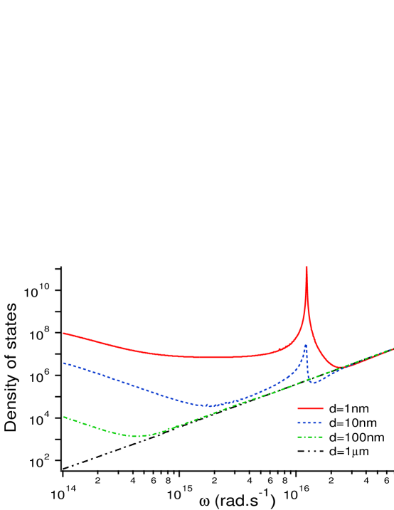
Figure 1: LDOS versus frequency at different heights above a semi-infinite sample of aluminum.

We plotted in Fig.1 the LDOS $\rho({\bf r},\omega)$ in the near UV-near IR frequency domain at four different heights. We first note that the LDOS increases drastically when the distance to the material is reduced. As discussed in the previous paragraph, at large distance from the material, one retrieves the vacuum density of states. Note that at a given distance, it is always possible to find a sufficiently high frequency for which the corresponding wavelength is small compared to the distance so that a far-field situation is retrieved. When the distance to the material is reduced, additional modes are present: these are the evanescent modes that are confined close to the interface and that cannot be seen in the far field. Moreover, aluminum exhibits a resonance around $\omega=\omega_{p}/\sqrt{2}$. Below this frequency, the material supports resonant surface waves (surface-plasmon polaritons). Additional modes are therefore seen in the near field. This produces an increase of the LDOS close to the interface. The enhancement is particularly important at the resonant frequency which corresponds to $Re[\epsilon(\omega)]=-1$. This behavior is analogous to that previously described in Ref.Shchegrov for a SiC surface supporting surface-phonon polaritons. Also note that in the low frequency regime, the LDOS increases. Finally, Fig.1 shows that it is possible to have a LDOS smaller than that of vacuum at some particular distances and frequencies.

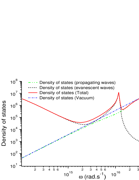
Figure 2: Density of states contributions due to the propagating and evanescent waves compared to the toatal density of states and the vacuum density of states. These quantities are calculated above an aluminum sample at a distance of 10 nm.

Figure 2 shows the propagating and evanescent waves contributions to the LDOS above an aluminum sample at a distance of 10 nm. The propagating contribution is very similar to that of the vacuum LDOS. As expected, the evanescent contribution dominates at low-frequency and around the surface-plasmon polariton resonance), where pure near-field contributions dominates.

We now turn to the comparison of $\rho(z,\omega)$ with the usual definition often encountered in the literature, which corresponds to $\rho^{E}(z,\omega)$. We plot in Fig.3 $\rho$, $\rho^{E}$ and $\rho^{H}$ above an aluminum surface at a distance $z=10nm$. In this figure, it is possible to identify three different domains for the LDOS behaviour. We note again that in the far-field situation (corresponding here to high frequencies i.e. $\lambda/2\pi\ll z$), the LDOS reduces to the vacuum situation. In this case $\rho(z,\omega)=2\rho^{E}(z,\omega)=2\rho^{H}(z,\omega)$. Around the resonance, the LDOS is dominated by the electric-field Green contribution. Conversely, at low frequencies, $\rho^{H}(z,\omega)$ dominates. Thus, Fig.3 shows that we have to be very careful when using the expression $\rho(z)=\rho^{E}(z,\omega)$. Above aluminum and at a distance $z=10nm$, this approximation is only valid on a small range between $\omega=10^{16}rad.s^{-1}$ and $\omega=1.5\times 10^{16}rad.s^{-1}$.

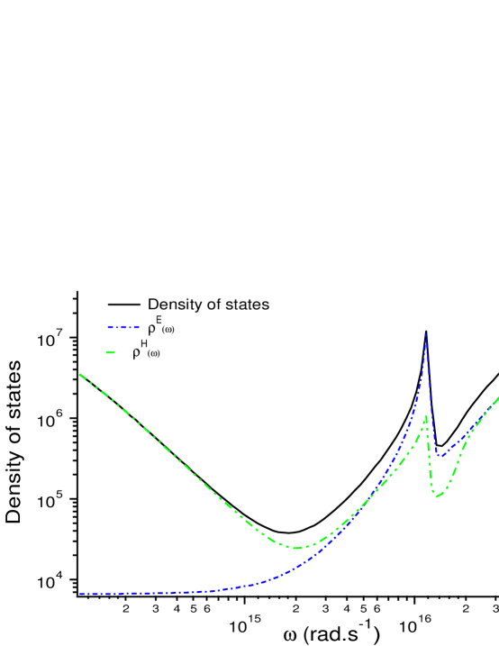
Figure 3: LDOS at a distance $z=10nm$ above a semi-infinite aluminum sample. Comparison with $\rho^{E}(\omega)$ and $\rho^{H}(\omega)$.

III.3 Asymptotic form of the LDOS in the near-field

In order to get more physical insight, we have calculated the asymptotic LDOS behaviour in the three regimes mentioned above. As we have already seen, the far-field regime ($\lambda/2\pi\ll d$) corresponds to the vacuum case. To study the near-field situation, we focus on the evanescent contribution as suggested by the results in Fig.2. When $\lambda=2\pi c/\omega\gg z$, the exponential term $\exp(-|p|\omega z/c)$ is small only for $\kappa\gg\lambda/(4\pi z)\gg 1$. In this (quasi-static) limit, the Fresnel reflection factors reduce to

$$\lim_{\kappa\rightarrow\infty}r^{s}_{12} = \frac{\epsilon-1}{4\kappa^{2}}$$ (15)

$$\lim_{\kappa\rightarrow\infty}r^{p}_{12} = \frac{\epsilon-1}{\epsilon+1}$$ (16)

Asymptotically, the expressions of $\rho^{E}(z,\omega)$ and $\rho^{H}(z,\omega)$ are

$$\rho^{E}(z,\omega) = \frac{\rho_{v}}{|\epsilon+1|^{2}}\frac{\epsilon^{{}^{\prime\prime}}}{4k_{0}^{3}z^{3}}$$ (17)

$$\rho^{H}(z,\omega) = \rho_{v}\left[\frac{\epsilon^{{}^{\prime\prime}}}{16k_{0}z}+\frac{\epsilon^{{}^{\prime\prime}}}{4|\epsilon+1|^{2}k_{0}z}\right]$$ (18)

At a distance $z=10nm$ above an aluminum surface, these asymptotic expressions matches almost perfectly with the full evanescent contributions ($\kappa>1$) of $\rho^{E}$ and $\rho^{H}$. These expressions also show that for a given frequency, one can always find a distance to the interface $z$ below which the dominant contribution to the LDOS will be the one due to the imaginary part of the electric-field Green function that varies like $(k_{0}z)^{-3}$. But for aluminum at a distance $z=10nm$, this is not the case for all frequencies. As we mentionned before, this is only true around the resonance. For example for low frequencies, and for $z=10nm$, the LDOS is actually dominated by $\rho_{v}\epsilon^{{}^{\prime\prime}}/(16k_{0}z)$.

III.4 Spatial oscillations of the LDOS

Let us now focus on the LDOS variations at a given frequency versus the distance $z$ to the interface. There are essentially three regimes. First, for as discussed previously, at distances much larger than the wavelength the LDOS is given by the vacuum expression $\rho_{v}$. The second regime is observed close to the interface where oscillations are observed. Indeed, at a given frequency, each incident plane wave on the interface can interfere with its reflected counterpart. This generate an interference pattern with a fringe spacing that depends on the angle and the frequency. Upon adding the contributions of all the plane waves over angles, the oscillating structure disappears except close to the interface. This leads to oscillations around distances on the order of the wavelength. This phenomenon is the electromagnetic analog of Friedel oscillations that can be observed in the electronic density of states near the interfaces ashcroft ; Harrisson . As soon as the distance becomes small compared to the wavelength, the phase factors $\exp(2ip\omega z/c)$ in Eq. (13) are equal to unity. For a highly reflecting material, the real part of the reflecting coefficients are negative so that the LDOS decreases while approaching the surface. These two regimes are clearly observed for aluminum in Fig. 4. The third regime is observed at small distances as seen in Fig. 4. The evanescent contribution dominates and ultimately the LDOS always increases as $1/z^{3}$, following the behaviour found in Eq. (17). This is the usual quasi-static contribution that is always found at short distanceCarsten .

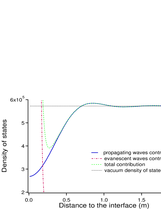
Figure 4: LDOS versus the distance $z$ from an aluminum-vacuum interface at the aluminum resonant frequency.

At a frequency slightly smaller than the resonant frequency, surface waves are excited on the surface. These additional modes increase the LDOS according to an exponential law as seen in Fig. 5, a behavior which was already found for thermally emitted fields Carminati ; Carsten . At low frequency, the LDOS dependance is given by Eq.(18). The $1/z$ magnetic term dominates because the $1/|\epsilon+1|^{2}$ takes large values. The $1/z^{3}$ contribution equals the $1/z$ contribution for distances much smaller than the nanometer scale, a distance for which the model is no longer valid.

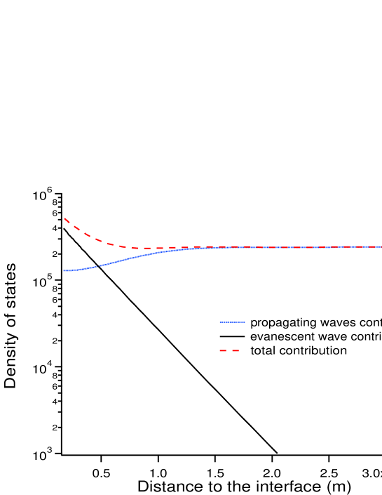
Figure 5: LDOS versus the distance $z$ from an aluminum-vacuum interface at frequency $\omega=8$ 10¹⁵ rad.s^-1.

The main results of this section can be summarized as follows. The LDOS of the electromagnetic field can be unambiguously and properly defined from the local density of electromagnetic energy in a vacuum above a sample at temperature $T$ in equilibrium. The LDOS can always be written as a function of the electric-field Green function only, but is in general not proportionnal to the trace of its imaginary part. An additional term proportional to the trace of the imaginary part of the magnetic-field Green function is present in the far-field and at low frequencies. At short distance from the surface of a material supporting surface modes (plasmon or phonon-polaritons), the LDOS presents a resonance at frequencies such that $Re[\epsilon(\omega)]=-1$. Close to this resonance, the approximation $\rho(z,\omega)=\rho^{E}(z,\omega)$ holds. In the next section, we discuss how the LDOS can be measured.

IV Measurement of the LDOS

IV.1 Near-field thermal emission spectroscopy with an apertureless SNOM

In this section we shall consider how the LDOS can be measured using a SNOM. We consider a frequency range where $\rho$ is dominated by the electric contribution $\rho^{E}$. We note that for an isotropic dipole, a lifetime measurement yields the LDOS as discussed by Wijnands et al. MartinMoreno . However, if the dipole has a fixed orientation ${\bf x}$, the lifetime is proportionnal to $G_{xx}$ and not to the trace of ${\stackrel{{\scriptstyle\leftrightarrow}}{{\bf G}}}$. In order to achieve a direct SNOM measurement of the LDOS, we have to fulfill two requirements. First, all the modes must be excited. The simplest way to achieve this is to use the thermally emitted radiation by a body at equilibrium. The second requirement is to have a detector with a flat response to all modes. To analyse this problem we use a formalism recently introduced.

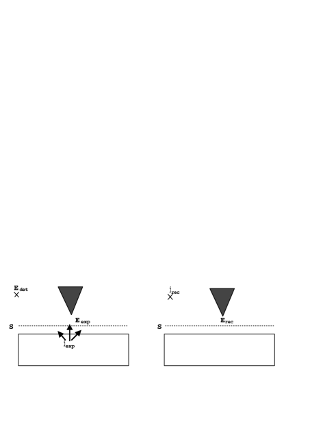
Figure 6: Scheme of a scanning near-field optical microscope measuring a thermally emitted field. (a): experimental situation. (b): reciprocal (fictitious) situation.

We consider a SNOM working in the detection mode, and detecting the electromagnetic field thermally emitted by a sample held at a temperature $T$. The system is depicted in Fig. 6. The microscope tip is scanned at close proximity of the interface separating the solid body from a vacuum. The signal is measured in the far field, by a point detector sensitive to the energy flux carried by the electromagnetic field. We assume that an analyzer is placed in front of the detector (polarized detection). The direction of polarization of the analyzer is along the direction of the vector ${\bf j}_{rec}$. If the solid angle $d\Omega$ under which the detector is seen from the tip is small (a condition we assume for simplicity), the signal ${\langle S(\omega)\rangle}$ at the detector, at a given frequency $\omega$, reads

$${\langle S(\omega)\rangle}=\frac{\epsilon_{0}c}{2}\left|{\bf E}_{d}\right(\omega)|^{2}r^{2}d\Omega$$ (19)

where $\epsilon_{0}$ is the permittivity of vacuum, $c$ is the speed of light in vacuum, $r$ is the distance between the tip and the detector, and ${\bf E}_{d}$ is the electric field at the position of the detector. Let us denote by ${\bf E}_{exp}$ (experimental field) the thermal field, emitted by the sample, in the gap region between the tip and the sample. This field can be, in principle, calculated following the approach recently used in Carminati ; Shchegrov . For simplicity, we shall neglect the thermal emission from the tip itself (which is assumed to be cold) compared to that of the heated sample. But we do not need, at this stage, to assume a weak coupling between the tip and the sample. In particular, in the expressions derived in this section, the experimental field ${\bf E}_{exp}$ is the field emitted by the sample alone, in the presence of the detecting tip. Following the approach of Porto , based on the reciprocity theorem of electromagnetism reviewSNOM , an exact relationship between the signal ${\langle S(\omega)\rangle}$ and the experimental field ${\bf E}_{exp}$ can be established. It can be shown that the signal is given by an overlapping integral.

To proceed, one considers a fictitious situation in which the sample is removed, and a point source, represented by a monochromatic current ${\bf j}_{rec}$ oscillating at frequency $\omega$, is placed at the position of the detector (see Fig. 6(b)). The orientation of this reciprocal source is chosen along the direction of polarization of the analyzer used in the experimental situation. The field created around the tip in this reciprocal situation is denoted by ${\bf E}_{rec}$. Using the reciprocity theorem, the field at the detector can be written Porto :

$${\bf E}_{d}(\omega)\cdot{\bf j}_{rec}=\frac{-2i}{\mu_{0}\omega}\int_{S}\frac{\partial{\bf E}_{rec}({\bf R},z,\omega)}{\partial z}\cdot{\bf E}_{exp}({\bf R},z,\omega)d{\bf R}$$ (20)

where the integration is performed in a plane $z=z_{0}$ between the tip and the sample and ${\bf R}=(x,y)$ are the coordinates along this plane. Equation (20) connects the field above the surface ${\bf E}_{exp}$ to the field in the detector ${\bf E}_{d}$ along the direction of the analyzer. Note that the reciprocal field ${\bf E}_{rec}$ encodes all the information about the detection system (tip and collection optics). Reporting the expression of the field at the detector (20) in (19), one finds the expression for the measured signal:

$${\langle S(\omega)\rangle}=\frac{\epsilon_{0}c}{8\pi^{2}}\int_{S}\!\!\int_{S}H_{ij}({\bf R},{\bf R}^{\prime},z,\omega)W_{ij}({\bf R},{\bf R}^{\prime},z,\omega)d{\bf R}d{\bf R}^{\prime}\ .$$ (21)

Equation (21) establishes a linear relationship between the signal and the cross-spectral density tensor $W_{ij}$ of the electric field defined by

$$\langle E_{exp,i}({\bf R},z,\omega)E_{exp,j}^{*}({\bf R}^{\prime},z,\omega^{\prime})\rangle=W_{ij}({\bf R},{\bf R}^{\prime},z,\omega)\,\delta(\omega-\omega^{\prime})\ .$$ (22)

The response function $H_{ij}$ only depends on the detection system (in particular the tip geometry and composition), and is given by

$$H_{ij}({\bf R},{\bf R}^{\prime},\omega)=\frac{\partial{\bf E}_{rec,i}({\bf R},z,\omega)}{\partial z}\frac{\partial{\bf E}_{rec,j}({\bf R}^{\prime},z,\omega)}{\partial z}\ .$$ (23)

The cross-spectral density tensor $W_{ij}$ describes the electric-field spatial correlation at a given frequency $\omega$. For the thermal emission situation considered here, it depends only on the dielectric constant, on the geometry and on the temperature of the sample.

Equation (21) is a general relationship between the signal and the cross-spectral density tensor. It is non-local and strongly polarization dependent. This shows that one do not measure in general a quantity which is proportional to $W_{kk}({\bf r},{\bf r},\omega)$, and thus to $\rho^{E}({\bf r},\omega)$. Nevertheless Eq. (21) suggested that $\rho^{E}({\bf r},\omega)$ can be recovered if the response function $H_{ij}$ is localized. Indeed, in that case the signal is proportional to $W_{ij}({\bf R},{\bf R},z,\omega)$, thus to $\rho^{E}({\bf r},\omega)$. As shown in the next section, a dipole tip (small sphere) would exhibit such a response function.

IV.2 Detection of the LDOS by an ideal point-dipole probe

Let us see what would be measured by an ideal probe consisting of a single electric dipole described by a polarizability $\alpha(\omega)$. Note that such a probe was proposed as a model for the uncoated dielectric probe sometimes used in photon scanning tunneling microscopy (PSTM), and gives good qualitative prediction VanLabeke . We assume that the thermally emitting medium occupies the half-space $z<0$, and that the probe is placed at a point ${\bf r}_{t}$. As in the preceding section, the detector placed in the far field measures the field intensity at a given point ${\bf r}_{d}$, through an analyser whose polarization direction is along the vector ${\bf j}_{rec}$. In this case, Eq. (20) simplifies to read

$${\bf j}_{rec}\cdot{\bf E}_{d}=\alpha(\omega)\,\frac{\omega^{2}}{4\pi c^{2}}\,\frac{\exp(ik|{\bf r}_{d}-{\bf r}_{t}|)}{|{\bf r}_{d}-{\bf r}_{t}|}\,{\bf j}_{rec}\cdot{\stackrel{{\scriptstyle\leftrightarrow}}{{\bf h}}}({\bf u}_{d})\cdot{\bf E}_{exp}({\bf r}_{t},\omega)$$ (24)

where $k=\omega/c$, ${\bf u}_{d}=({\bf r}_{d}-{\bf r}_{t})/|{\bf r}_{d}-{\bf r}_{t}|$ is the unit vector pointing from the probe towards the detector and ${\stackrel{{\scriptstyle\leftrightarrow}}{{\bf h}}}({\bf u}_{d})={\stackrel{{\scriptstyle\leftrightarrow}}{{\bf I}}}-{\bf u}_{d}{\bf u}_{d}$ is the dyadic operator which projects a vector on the direction transverse to ${\bf u}_{d}$, ${\stackrel{{\scriptstyle\leftrightarrow}}{{\bf I}}}$ being the unit dyadic operator. The dyadic ${\stackrel{{\scriptstyle\leftrightarrow}}{{\bf h}}}({\bf u}_{d})$ being symmetric, the scalar product in the right-hand side in Eq. (24) can be transformed using the equality ${\bf j}_{rec}\cdot{\stackrel{{\scriptstyle\leftrightarrow}}{{\bf h}}}({\bf u}_{d})\cdot{\bf E}_{exp}({\bf r}_{t},\omega)={\bf E}_{exp}({\bf r}_{t},\omega)\cdot{\stackrel{{\scriptstyle\leftrightarrow}}{{\bf h}}}({\bf u}_{d})\cdot{\bf j}_{rec}$. Finally, the signal at the detector writes

$$\langle S\rangle=|\alpha(\omega)|^{2}\frac{\omega^{4}}{4\pi c^{4}}\,\mathrm{d}\Omega\,\sum_{i,j}A_{i}A_{j}^{*}W_{ij}({\bf r}_{t},{\bf r}_{t},\omega)$$ (25)

where ${\bf A}={\stackrel{{\scriptstyle\leftrightarrow}}{{\bf h}}}({\bf u}_{d})\cdot{\bf j}_{rec}$ is a vector depending only on the detection conditions (direction and polarization). Note that if ${\bf j}_{rec}$ is transverse with respect to the direction ${\bf u}_{d}$, which is approximately the case in many experimental set-ups, then one simply has ${\bf A}={\bf j}_{rec}$.

Equation (25) shows that with an ideal probe consisting of a signal dipole (with an isotropic polarizability $\alpha(\omega)$, one locally measures the cross-spectral density tensor at the position ${\bf r}_{t}$ of the tip. Nevertheless, polarization properties of the detection still exists so that the trace of $W_{ij}$, and therefore $\rho^{E}({\bf r},\omega)$, is not directly measured. A possibility of measuring the trace would be to measure a signal $\langle S_{1}\rangle$ in the direction normal to the surface with an unpolarized detection, and a signal $\langle S_{2}\rangle$ in the direction parallel to the surface, with an analyzer in the vertical direction. $\langle S_{1}\rangle$ would be a sum of the two signals obtained with ${\bf j}_{rec}$ along the $x$-direction and along the $y$-direction. $\langle S_{2}\rangle$ would correspond to the signal measured with ${\bf j}_{rec}$ along the $z$-direction. Using Eq. (25), we see that the signal $\langle S\rangle=\langle S_{1}\rangle+\langle S_{2}\rangle$ is proportional to the trace $W_{kk}({\bf r}_{t},{\bf r}_{t},\omega)$, and thus to $\rho^{E}({\bf r},\omega)$. Measuring the thermal spectrum of emission with an apertureless SNOM which probe is dipolar is thus a natural way to achieve the measurement of $\rho^{E}({\bf r},\omega)$. Close to the material resonances, i.e in the frequency domain where $\rho^{E}({\bf r},\omega)$ matches $\rho({\bf r},\omega)$, such a near-field thermal emission spectrum gives the electromagnetic LDOS.

IV.3 Analogy with scanning (electron) tunneling microscopy

The result in this section shows that a SNOM measuring the thermally emitted field with a dipole probe (for example a sphere much smaller than the existing wavelengths) measures the electromagnetic LDOS of the sample in the frequency range situated around the resonant pulsation. As discussed above, the measured LDOS is that of the modes which can be excited in the thermal emission process in a cold vacuum. This result was obtained from Eq. (20) assuming a weak tip-sample coupling, i.e., the experimental field is assumed to be the same with or without the tip.

The same result could be obtained starting from the generalized Bardeen formula derived in ref.Carminati2 . Using this formalism for a dipole probe, one also ends up with Eq. (25), which explicitly shows the linear relationship between the signal and $\rho^{E}({\bf r},\omega)$. This derivation is exactly the same as that used in the Tersoff and Haman theory of the STM Tersoff . This theory showed, in the weak tip-sample coupling limit, that the electron-tunneling current measured in STM was proportional to the electronic LDOS of the sample, at the tip position, and at the Fermi energy. This result, although obtained under some approximations, was a breakthrough in understanding the STM signal. In the case of near-field optics, the present discussion, together with the use of the generalized Bardeen formula Carminati2 , shows that under similar approximations, a SNOM using an ideal dipole probe and measuring the field thermally emitted by the sample is the real optical analog to the electron STM. We believe that this situation provides for SNOM a great potential for local solid-surface spectroscopy, along the directions opened by STM.

IV.4 Could the LDOS be detected by standard SNOM techniques ?

Before concluding, we will discuss the ability of standard SNOM techniques (by “standard” we mean techniques using laser-light illumination) to image the electromagnetic LDOS close to a sample. Recent experiments Chicanne have shown that an illumination-mode SNOM using metal-coated tips and working in transmission produce images which reproduce calculated maps of $\rho^{E}({\bf r},\omega)$ (which is the adopted definition of the LDOS in this experimental work, see also Colas ). We shall now show that this operating mode bear strong similarites to that corresponding to a SNOM working in collection mode, and measuring thermally emitted fields. This will explain why the images reproduce (at least qualitatively) the electric LDOS $\rho^{E}({\bf r},\omega)$.

Let us first consider a collection-mode technique, in which the sample (assumed to be transparent) is illuminated in transmission by a monochromatic laser with frequency $\omega$, and the near-field light is collected by a local probe. If we assume the illuminating light to be spatially incoherent and isotropic in the lower half-space (with all incident directions included), then this illumination is similar to that produced by thermal fluctuations (except that only the modes corresponding to the frequency $\omega$ are actually excited). Note that this mode of illumination corresponds to that proposed in Ref. Carminati3 . This similarity, together with the discussion in the precedding paragraph, allows to conclude that under these operating conditions, a collection-mode SNOM would produce images which closely resemble the electric LDOS $\rho^{E}({\bf r},\omega)$.

We now turn to the discussion of images produced using an illumination-mode SNOM, as that used in Ref. Chicanne . The use of the reciprocity theorem allows to derive an equivalence between illumination and collection-mode configurations, as shown in Ref. Mendez . Starting from the collection-mode instrument described above, the reciprocal illumination-mode configuration corresponds to a SNOM working in transmission, the light being collected by an integrating sphere over all possible transmission directions (including those below and above the critical angle). Under such conditions, the illumination-mode SNOM produces exactly the same image as the collection-mode SNOM using isotropic, spatially incoherent and monochromatic illumination. This explains why this instrument is able to produce images which closely follow the electric LDOS $\rho^{E}({\bf r},\omega)$. Finally, note that in Ref. Chicanne , the transmitted light is collected above the critical angle only, which in principle should be a drawback regarding the LDOS imaging. In these experiments, it seems that the interpretation of the images as maps of the electric LDOS remains nevertheless qualitatively correct, which shows that in this case, the main contribution to the LDOS comes from modes with wavevector corresponding to propagation directions above the critical angle.

V Conclusion

In this paper, we have introduced a defintion of the electromagnetic LDOS $\rho({\bf r},\omega)$. We have shown that it is fully determined by the electric-field Green function, but that in general it does not reduce to the trace of its imaginary part $\rho^{E}({\bf r},\omega)$. We have studied the LDOS variations versus the distance to a material surface and have explicitly shown examples in which the LDOS deviates from $\rho^{E}({\bf r},\omega)$. Nevertheless, we have shown that around the material resonances (surface polaritons), the near-field LDOS reduces to $\rho^{E}({\bf r},\omega)$. Measuring the LDOS with an apertureless SNOM using a point-dipole tip should be feasible. The principle of the measurement is to record a near-field thermal emission spectrum. Under such condition, the instrument behaves as the optical analog of the STM, in the weak-coupling regime, which is known to measure the electronic LDOS on a metal surface. Finallly, we have discussed recent standard SNOM experiments in which the LDOS seems to be qualitatively measured. Using general arguments, we have discussed the relevance of such measurements and compared them to measurements based on thermal-emission spectroscopy.

Appendix A Calculation of the field at the detector for an ideal point-dipole probe

Let ${\bf e}_{rec}({\bf K})$ and ${\bf e}_{exp}({\bf K})$ be the bidimensional Fourier component of ${\bf E}_{rec}({\bf r})$ and ${\bf E}_{exp}({\bf r})$. In the configuration chosen in our problem the reciprocal field propagates to the negative $z$ whereas the experimental fields propagates to the positive $z$. Thus

$${\bf E}_{rec}({\bf r})=\int{\bf e}_{rec}({\bf K})\exp[i({\bf K}.{\bf R}-\gamma({\bf K})z)]d{\bf K}$$ (26)

$${\bf E}_{exp}({\bf r})=\int{\bf e}_{exp}({\bf K})\exp[i({\bf K}.{\bf R}+\gamma({\bf K})z)]d{\bf K}$$ (27)

where $\gamma({\bf K})=\sqrt{\omega^{2}/c^{2}-K^{2}}$. Putting Eqs. (26) and (27) into Eq.(20) gives

$${\bf E}_{d}(\omega)\cdot{\bf j}_{rec}=-\frac{8\pi^{2}}{\omega\mu_{0}}\int\gamma({\bf K}){\bf e}_{rec}(-{\bf K})\cdot{\bf e}_{exp}({\bf K})d{\bf K}$$ (28)

${\bf e}_{exp}(K)$ can be evaluated by calculating the field ${\bf E}_{exp}({\bf r})$. This last field is the field radiated by the reciprocal current ${\bf j}_{rec}$ and diffused by the ideal probe. It can also be seen as the field radiated by the dipole induced at the position ${\bf r}_{t}=({\bf R}_{t},z_{t})$ of the probe. If ${\bf p}$ is the dipole induced at the position of the ideal probe, the reciprocal field at a position situated below the probe writes:

$${\bf E}_{rec}({\bf r})=\mu_{0}\omega^{2}{\stackrel{{\scriptstyle\leftrightarrow}}{{\bf G}}}({\bf r},{\bf r}_{t})\cdot{\bf p}$$

$$=\frac{i\mu_{0}\omega^{2}}{8\pi^{2}}\int\frac{d^{2}Ke^{i[{\bf K}.({\bf R}-{\bf R}_{t})+\gamma(z_{t}-z)]}}{\gamma}\left[{\stackrel{{\scriptstyle\leftrightarrow}}{{\bf I}}}-\frac{{\bf k}{\bf k}}{k_{0}^{2}}\right]\cdot{\bf p}$$ (29)

where $k_{0}^{2}=\omega^{2}/c^{2}$. Comparing this expression and (26),then

$${\bf e}_{rec}({\bf K})=\frac{i\mu_{0}\omega^{2}}{8\pi^{2}\gamma({\bf K})}e^{i(-{\bf K}.{\bf R}_{t}+\gamma({\bf K})z_{t})}{\stackrel{{\scriptstyle\leftrightarrow}}{{\bf h}}}({\bf k}^{-})\cdot{\bf p}$$ (30)

where ${\bf k}^{-}=({\bf K},-\gamma)$. Furthermore, using the fact that ${\stackrel{{\scriptstyle\leftrightarrow}}{{\bf h}}}({\bf k})={\stackrel{{\scriptstyle\leftrightarrow}}{{\bf h}}}(-{\bf k})$ and defining ${\bf k}^{+}=({\bf K},\gamma)$

$${\bf e}_{rec}(-{\bf K})=\frac{i\mu_{0}\omega^{2}}{8\pi^{2}\gamma}e^{i({\bf K}.{\bf R}_{t}+\gamma z_{t})}{\stackrel{{\scriptstyle\leftrightarrow}}{{\bf h}}}({\bf k}^{+})\cdot{\bf p}$$ (31)

Let us denote ${\bf E}({\bf j}{rec}\rightarrow{\bf r}_{t})$ the field radiated by the reciprocal current in ${\bf r}_{t}$. The dipole induced then writes ${\bf p}=\alpha(\omega)\epsilon_{0}{\bf E}({\bf j}{rec}\rightarrow{\bf r}_{t})$ and

$${\bf E}({\bf j}{rec}\rightarrow{\bf r}_{t})=\frac{i\omega\mu_{0}}{4\pi}\frac{e^{i|{\bf r}_{d}-{\bf r}_{t}|}}{|{\bf r}_{d}-{\bf r}_{t}|}{\stackrel{{\scriptstyle\leftrightarrow}}{{\bf h}}}({\bf u}_{d})\cdot{\bf j}_{rec}$$ (32)

Using the fact that for all dyadic ${\stackrel{{\scriptstyle\leftrightarrow}}{{\bf A}}}$ and for all vector ${\bf a}$ and ${\bf b}$

$$[{\stackrel{{\scriptstyle\leftrightarrow}}{{\bf A}}}\cdot{\bf a}]\cdot{\bf b}={\bf a}\cdot[{\stackrel{{\scriptstyle\leftrightarrow}}{{\bf A}}}^{T}\cdot{\bf b}]$$ (33)

that ${\stackrel{{\scriptstyle\leftrightarrow}}{{\bf h}}}$ is a symetric dyadic (${\stackrel{{\scriptstyle\leftrightarrow}}{{\bf h}}}={\stackrel{{\scriptstyle\leftrightarrow}}{{\bf h}}}^{T}$), that ${\bf e}_{exp}({\bf K})$ is transverse to the direction ${\bf k}^{+}$ and the definition of ${\bf E}_{exp}({\bf r})$.

$${\bf j}_{rec}\cdot{\bf E}_{d}=\alpha(\omega)\,\frac{\omega^{2}}{4\pi c^{2}}\,\frac{\exp(ik|{\bf r}_{d}-{\bf r}_{t}|)}{|{\bf r}_{d}-{\bf r}_{t}|}\,{\bf j}_{rec}\cdot{\stackrel{{\scriptstyle\leftrightarrow}}{{\bf h}}}({\bf u}_{d})\cdot{\bf E}_{exp}({\bf r}_{t},\omega)$$ (34)

References

- (1) N. G Van Kampen, B.R.A. Nijboer and K. Schram, Phys. Lett., 26 A, 307 (1968).
- (2) E. Gerlach, Phys. Rev. B, 4, 393 (1971).
- (3) J.-B. Pendry, J. Phys.: Condens. Matter, 9, 10301 (1997).
- (4) J.P Mulet, K. Joulain, R. Carminati, and J.-J. Greffet, Microscale Thermophysical Engineering, 6, 209-222 (2002).
- (5) R. Carminati and J.-J. Greffet, Phys. Rev. Lett. 82, 1660 (1999).
- (6) E.N. Economou, Green’s Functions in Quantum Physics (Springer, Berlin, 1983).
- (7) W.A. Harrison, Solid State Theory, (Dover, New-York, 1980).
- (8) J. Tersoff and D.R. Hamann, Phys. Rev. B 31, 805 (1985).
- (9) M.F Crommie, C.P. Lutz and D.M Eigler, Science, 262, 218 (1993).
- (10) F. Wijnands, J.B. Pendry, F.J. Garcia-Vidal, P.J. Roberts and L. Martin Moreno, Optical and Quantum Electronics, 29 199 (1997).
- (11) R. Carminati and J.J Sáenz, Phys. Rev. Lett. 84, 5156 (2000).
- (12) D.W. Pohl and D. Courjon (eds.), Near-Field Optics (Kluwer, Dordrecht, 1993); M.A. Paesler and P.J. Moyer, Near Field Optics: Theory, Instrumentation and Applications (Wiley-Interscience, New-York, 1996); M. Ohtsu (ed.), Near-field Nano/Atom Optics and Technology (Springer-Verlag, Tokyo, 1998).
- (13) P.J. Moyer, C.L. Jahnckle, M.A. Paesler, R.C. Reddick and R.J. Warmack, Phys. Lett. A 45, 343 (1990).
- (14) C.L. Jahnckle, M.A. Paesler and H.D. Hallen, Appl. Phys. Lett. 67, 2483 (1995); J. Grausem, B. Humbert, A. Burenau, J. Oswalt, Appl. Phys. Lett. 70, 1671 (1997).
- (15) E.J. Sanchez, L. Novotny and X. S. Xie, Phys. Rev. Lett. 82, 4014 (1999).
- (16) F. Zenhausern, M.P. O’Boyle and H.K. Wickramasinghe, Appl. Phys. Lett. 65, 1623 (1994); Y. Inouye and S. Kawata, Opt. Lett. 19, 159 (1994); P. Gleyzes, A.C. Boccara and R. Bachelot, Ultramicroscopy 57, 318 (1995).
- (17) A. Lahrech, R. Bachelot, P. Gleyzes and A.C. Boccara, Appl. Phys. Lett. 71, 575 (1997).
- (18) B. Knoll and F. Keilman, Nature 399, 134 (1999).
- (19) S.M. Rytov, Yu. A. Kravtsov and V.I. Tatarskii, Principles of Statistical Radiophysics , vol. 3, (Springer-Verlag, Berlin, 1989).
- (20) J.E. Sipe, J. Opt. Soc. Am. B, 4, 481 (1987).
- (21) C. Henkel, S. Pötting and M. Wilkens, Appl. Phys. B 69, 379 (1999).
- (22) G. Colas des Francs, C. Girard, J.-C. Weeber, C. Chicanne, T. David, A. Dereux and D.Peyrade, Phys. Rev. Lett., 86, 4950 (2001).
- (23) C. Chicanne, T. David, R. Quidant, J.C. Weeber, Y. Lacroute, E. Bourillot, A.Dereux, G. Colas des Francs and C. Girard, Phys. Rev. Lett., 88, 097402 (2002).
- (24) A.V. Shchegrov, K. Joulain, R. Carminati and J.-J. Greffet, Phys. Rev. Lett. 85, 1548 (2000).
- (25) G. S. Agarwal, Phys. Rev. A 11, 231 (1975).
- (26) C. Henkel, K. Joulain, R. Carminati and J.-J. Greffet, Opt. Comm. 186, 57 (2000).
- (27) E.D. Palik, Handbook of Optical Constants, (Academic Press Inc., San Diego, 1985).
- (28) A. Ashcroft and D. Mermin, Solid Sate physics, (Saunders College, Philadelphia, 1976).
- (29) J.A. Porto, R. Carminati and J.-J. Greffet, J. Appl. Phys. 88, 4847 (2000).
- (30) J.-J. Greffet and R. Carminati, Prog. Surf. Sci. 56, 133 (1997).
- (31) D. Van Labeke and D. Barchiesi, J. Opt. Soc. Am. A 10, 2193 (1993).
- (32) L. Aigouy, F.X. Andreani, A.C. Boccara, J.C. Rivoal, J.A. Porto, R. Carminati, J.-J. Greffet and R. Megy, Appl. Phys. Lett. 76, 397 (2000).
- (33) R. Carminati, J.-J. Greffet, N. García and M. Nieto-Vesperinas, Opt. Lett. 21, 501 (1996).
- (34) E.R. Méndez, J.-J. Greffet and R. Carminati, Opt. Commun. 142, 7 (1997).