.

Abstract

The new Process Physics provides a new explanation of space as a quantum foam system in which gravity is an inhomogeneous flow of the quantum foam into matter. An analysis of various experiments demonstrates that absolute motion relative to space has been observed experimentally by Michelson and Morley, Miller, Illingworth, Torr and Kolen, and by DeWitte. The Dayton Miller and Roland DeWitte data also reveal the in-flow of space into matter which manifests as gravity. The in-flow also manifests turbulence and the experimental data confirms this as well, which amounts to the observation of a gravitational wave phenomena. The Einstein assumptions leading to the Special and General Theory of Relativity are shown to be falsified by the extensive experimental data. Contrary to the Einstein assumptions absolute motion is consistent with relativistic effects, which are caused by actual dynamical effects of absolute motion through the quantum foam, so that it is Lorentzian relativity that is seen to be essentially correct.

Key words: Process Physics, quantum foam, quantum

gravity, absolute motion

1 Introduction

The new Process Physics [1, 2, 3, 4, 5, 6, 7, 8, 9, 10, 11, 12, 13] provides a new explanation of space as a quantum foam system in which gravity is an inhomogeneous flow of the quantum foam into matter. Here an analysis of data from various experiments demonstrates that absolute motion relative to space has been observed by Michelson and Morley, Miller, Illingworth, Torr and Kolen, and by DeWitte, contrary to common belief within physics that absolute motion has never been observed. The Dayton Miller and Roland DeWitte data also reveal the in-flow of space into matter which manifests as gravity. The experimental data suggests that the in-flow manifest turbulence, which amounts to the observation of a gravitational wave phenomena. The Einstein assumptions leading to the Special and General Theory of Relativity are shown to be falsified by the extensive experimental data.

Contrary to the Einstein assumptions absolute motion is consistent with relativistic effects, which are caused by actual dynamical effects of absolute motion through the quantum foam. Lorentzian relativity is seen to be essentially correct.

This paper is a condensed version of certain sections of Cahill [1].

2 Detection of Absolute Motion

2.1 Space and Absolute Motion

Absolute motion is motion relative to space itself. It turns out that Michelson and Morley in their historic experiment of 1887 did detect absolute motion, but rejected their own findings because using Galilean relativity the determined speed of some 8 km/s was less than the 30 km/s orbital speed of the Earth. The data was clearly indicating that the theory for the operation of the Michelson interferometer was not adequate. Rather than reaching this conclusion Michelson and Morley came to the incorrect conclusion that their results amounted to the failure to detect absolute motion. This had an enormous impact on the deveopment of physics, for as is well known Einstein adopted the absence of absolute motion effects as one of his fundamnetal assumptions. By the time Miller had finally figured out how to use and properly analyse data from his Michelosn interferometer absolute motion had become a forbidden concept within physics, as it still is at present. The experimental observations by Miller and others of absolute motion has continued to be scorned and rejected by the physics community. Unfortunately as well as revealing absolute motion the experimental data also reveals evidence in support of a new theory of gravity.

2.2 Theory of the Michelson Interferometer

Figure 1: Schematic diagrams of the Michelson Interferometer, with beamsplitter/mirror at $A$ and mirrors at $B$ and $C$, on equal length arms when parallel, from $A$. $D$ is a quantum detector (not drawn in (b)) that causes localisation of the photon state by a collapse process. In (a) the interferometer is at rest in space. In (b) the interferometer is moving with speed $v$ relative to space in the direction indicated. Interference fringes are observed at the quantum detector $D$. If the interferometer is rotated in the plane through $90^{o}$, the roles of arms $AC$ and $AB$ are interchanged, and during the rotation shifts of the fringes are seen in the case of absolute motion, but only if the apparatus operates in a gas. By counting fringe changes the speed $v$ may be determined.

We now show for the first time in over 100 years how the three key effects together permit the Michelson interferometer [14] to reveal the phenomenon of absolute motion when operating in the presence of a gas, with the third effect only discovered in 2002 [9]. The main outcome is the derivation of the origin of the Miller $k^{2}$ factor in the expression for the time difference for light travelling via the orthogonal arms,

$$\Delta t=2k^{2}\frac{L|{\bf v}_{P}|^{2}}{c^{3}}\cos(2(\theta-\psi)).$$ (1)

Here ${\bf v}_{P}$ is the projection of the absolute velocity ${\bf v}$ of the interferometer through the quantum-foam onto the plane of the interferometer, where the projected velocity vector ${\bf v}_{P}$ has azimuth angle $\psi$ relative to the local meridian, and $\theta$ is the angle of one arm from that meridian. The $k^{2}$ factor is $k^{2}=n(n^{2}-1)$ where $n$ is the refractive index of the gas through which the light passes, $L$ is the length of each arm and $c$ is the speed of light relative to the quantum foam. This expression follows from three key effects: (i) the difference in geometrical length of the two paths when the interferometer is in absolute motion, as first realised by Michelson, (ii) the Fitzgerald-Lorentz contraction of the arms along the direction of motion, and (iii) that these two effects precisely cancel in vacuum, but leave a residual effect if operated in a gas, because the speed of light through the gas is reduced to $V=c/n$, ignoring here for simplicity any Fresnel-drag effects, see [1]. This is one of the aspects of the quantum foam physics that distinguishes it from the Einstein formalism. The time difference $\Delta t$ is revealed by the fringe shifts on rotating the interferometer. In Newtonian physics, that is with no Fitzgerald-Lorentz contraction, $k^{2}=n^{3}$, while in Einsteinian physics $k=0$ reflecting the fundamental assumption that absolute motion is not measurable and indeed has no meaning. The Special Relativity null effect for the interferometer is explicitly derived in [1]. So the experimentally determined value of $k$ is a key test of fundamental physics. Table 1 summarises the differences between the three fundamental theories in their modelling of time, space, gravity and the quantum, together with their distinctive values for the interferometer parameter $k^{2}$. For air $n=1.00029$, and so for process physics $k=0.0241$ and $k^{2}=0.00058$, which is close to the Einsteinian value of $k=0$, particularly in comparison to the Newtonian value of $k=1.0$. This small but non-zero $k$ value explains why the Michelson interferometer experiments gave such small fringe shifts. Fortunately it is possible to check the $n$ dependence of $k$ as one experiment [17] was done in Helium gas, and this has an $n^{2}-1$ value significantly different from that of air.

Theory	Time	Space	Gravity	Quantum	$k^{2}$
Newton	geometry	geometry	force	Quantum Theory	$n^{3}$
Einstein	curved geometry		curvature	Quantum Field Theory	0
Process	process	quantum	inhomogeneous	Quantum Homotopic	$n(n^{2}-1)$
		foam	flow	Field Theory

Table 1: Comparisons of Newtonian, Einsteinian and Process Physics.

In deriving (2) in the new physics it is essential to note that space is a quantum-foam system which exhibits various subtle features. In particular it exhibits real dynamical effects on clocks and rods. In this physics the speed of light is only $c$ relative to the quantum-foam, but to observers moving with respect to this quantum-foam the speed appears to be still $c$, but only because their clocks and rods are affected by the quantum-foam. As shown in [1] such observers will find that records of observations of distant events will be described by the Einstein spacetime formalism, but only if they restrict measurements to those achieved by using clocks, rods and light pulses, that is using the Einstein measurement protocol. However if they use an absolute motion detector then such observers can correct for these effects.

It is simplest in the new physics to work in the quantum-foam frame of reference. If there is a gas present at rest in this frame, such as air, then the speed of light in this frame is $V=c/n$. If the interferometer and gas are moving with respect to the quantum foam, as in the case of an interferometer attached to the Earth, then the speed of light relative to the quantum-foam is still $V=c/n$ up to corrections due to drag effects. Hence this new physics requires a different method of analysis from that of the Einstein physics. With these cautions we now describe the operation of a Michelson interferometer in this new physics, and show that it makes predictions different to that of the Einstein physics. Of course experimental evidence is the final arbiter in this conflict of theories.

As shown in Fig.2 the beamsplitter/mirror when at $A$ sends a photon $\psi(t)$ into a superposition $\psi(t)=\psi_{1}(t)+\psi_{2}(t)$, with each component travelling in different arms of the interferometer, until they are recombined in the quantum detector which results in a localisation process, and one spot in the detector is produced. Repeating with many photons reveals that the interference between $\psi_{1}$ and $\psi_{2}$ at the detector results in fringes. These fringes actually only appear if the mirrors are not quite orthogonal, otherwise the screen has a uniform intensity and this intensity changes as the interferometer is rotated, as shown in the analysis by Hicks [18]. To simplify the analysis here assume that the two arms are constructed to have the same lengths $L$ when they are physically parallel to each other and perpendicular to $v$, so that the distance $BB^{\prime}$ is $L\sin(\theta)$. The Fitzgerald-Lorentz effect in the new physics is that the distance $SB^{\prime}$ is $\gamma^{-1}L\cos(\theta)$ where $\gamma=1/\sqrt{1-v^{2}/c^{2}}$. The various other distances are $AB=Vt_{AB}$, $BC=Vt_{BC}$, $AS=vt_{AB}$ and $SC=vt_{BC}$, where $t_{AB}$ and $t_{BC}$ are the travel times. Applying the Pythagoras theorem to triangle $ABB^{\prime}$ we obtain

$$t_{AB}=\frac{2v\gamma^{-1}L\cos(\theta)+\sqrt{4v^{2}\gamma^{-2}L^{2}\cos^{2}(\theta)+4L^{2}(1-\frac{v^{2}}{c^{2}}\cos^{2}(\theta))(V^{2}-v^{2})}}{2(V^{2}-v^{2})}.$$ (2)

Figure 2: One arm of a Michelson Interferometer travelling at angle $\theta$ and velocity ${\bf v}$, and shown at three successive times: (i) when photon leaves beamsplitter at $A$, (ii) when photon is reflected at mirror $B$, and (iii) when photon returns to beamsplitter at $C$. The line $BB^{\prime}$ defines right angle triangles $ABB^{\prime}$ and $SBB^{\prime}$. The second arm is not shown but has angle $\theta+90^{o}$ to ${\bf v}$. Here ${\bf v}$ is in the plane of the interferometer for simplicity, and the azimuth angle $\psi=0$.

The expression for $t_{BC}$ is the same except for a change of sign of the $2v\gamma^{-1}L\cos(\theta)$ term, then

$$t_{ABC}=t_{AB}+t_{BC}=\frac{\sqrt{4v^{2}\gamma^{-2}L^{2}\cos^{2}(\theta)+4L^{2}(1-\frac{v^{2}}{c^{2}}\cos^{2}(\theta))(V^{2}-v^{2})}}{(V^{2}-v^{2})}.$$ (3)

The corresponding travel time $t^{\prime}_{ABC}$ for the orthogonal arm is obtained from (3) by the substitution $\cos(\theta)\rightarrow\cos(\theta+90^{0})=\sin(\theta)$. The difference in travel times between the two arms is then $\Delta t=t_{ABC}-t^{\prime}_{ABC}$. Now trivially $\Delta t=0$ if $v=0$, but also $\Delta t=0$ when $v\neq 0$ but only if $V=c$. This then would result in a null result on rotating the apparatus. Hence the null result of Michelson interferometer experiments in the new physics is only for the special case of photons travelling in vacuum for which $V=c$. However if the interferometer is immersed in a gas then $V<c$ and a non-null effect is expected on rotating the apparatus, since now $\Delta t\neq 0$. It is essential then in analysing data to correct for this refractive index effect. The above $\Delta t$ is the change in travel time when one arm is moved through angle $\theta$. The interferometer operates by comparing the change in the difference of the travel times between the arms, and this introduces a factor of 2. Then for $V=c/n$ we find for $v<<V$ that

$$\Delta t=2Ln(n^{2}-1)\frac{v^{2}}{c^{3}}\cos(2\theta)+\mbox{O}(v^{4}),$$ (4)

that is $k^{2}=n(n^{2}-1)$, which gives $k=0$ for vacuum experiments ($n=1$). So the Miller phenomenological parameter $k$ is seen to accommodate both the Fitzgerald-Lorentz contraction effect and the dielectric effect, at least for gases. This is very fortunate since being a multiplicative parameter a re-scaling of old analyses is all that is required. $\Delta t$ is non-zero when $n\neq 1$ because the refractive index effect results in incomplete cancellation of the geometrical effect and the Fitzgerald-Lorentz contraction effect. Of course it was this cancellation effect that Fitzgerald and Lorentz actually used to arrive at the length contraction hypothesis, but they failed to take the next step and note that the cancellation would be incomplete in the air operated Michelson-Morley experiment. In a bizarre development modern Michelson interferometer experiments, which use resonant cavities rather than interference effects, but for which the analysis here is easily adapted, and with the same consequences, are operated in vacuum mode. That denies these experiments the opportunity to see absolute motion effects. Nevertheless the experimentalists continue to misinterpret their null results as evidence against absolute motion. Of course these experiments are therefore restricted to merely checking the Fitzgerald-Lorentz contraction effect, and this is itself of some interest.

All data from gas-mode interferometer experiments, except for that of Miller, has been incorrectly analysed using only the first effect as in Michelson’s initial theoretical treatment, and so the consequences of the other two effects have been absent. Repeating the above analysis without these two effects we arrive at the Newtonian-physics time difference which, for $v<<V$, is

$$\Delta t=2Ln^{3}\frac{v^{2}}{c^{3}}\cos(2\theta)+\mbox{O}(v^{4}),$$ (5)

that is $k^{2}=n^{3}$. The value of $\Delta t$, which is typically of order $10^{-17}s$ in gas-mode interferometers corresponding to a fractional fringe shift, is deduced from analysing the fringe shifts, and then the speed $v_{M}$ has been extracted using (5), instead of the correct form (4) or more generally (2). However it is very easy to correct for this oversight. From (4) and (5) we obtain for the corrected absolute (projected) speed $v_{P}$ through space, and for $n\approx 1^{+}$,

$$v_{P}=\frac{v_{M}}{\sqrt{n^{2}-1}}.$$ (6)

For air the correction factor in (6) is significant, and even more so for Helium.

2.3 The Michelson-Morley Experiment: 1887

Michelson and Morley reported that their interferometer experiment in 1887 gave a ‘null-result’ which since then, with rare exceptions, has been claimed to support the Einstein assumption that absolute motion has no meaning. However to the contrary the Michelson-Morley published data [15] shows non-null effects, but much smaller than they expected. They made observations of thirty-six $360^{0}$ turns using an $L=11$ meter length interferometer operating in air in Cleveland (Latitude $41^{0}30^{\prime}$N) with six turns near $12\!:\!\!00$ hrs ($7\!\!:\!\!00$ hrs ST) on each day of July 8, 9 and 11, 1887 and similarly near $18\!:\!\!00$ hrs ($13\!\!:\!\!00$ hrs ST) on July 8, 9 and 12, 1887. Each turn took approximately 6 minutes as the interferometer slowly rotated floating on a tank of mercury. They published and analysed the average of each of the 6 data sets. The fringe shifts were extremely small but within their observational capabilities.

Figure 3: Plot of micrometer readings for July 11 $12\!\!:\!\!00$ hr ($7\!\!:\!\!00$ ST) showing the absolute motion induced fringe shifts superimposed on the uniform temperature induced fringe drift.

local	16	1	2	3	4	5	6	7
time	8	9	10	11	12	13	14	15	16
12:00hr	27.3	23.5	22.0	19.3	19.2	19.3	18.7	18.9
July 11	16.2	14.3	13.3	12.8	13.3	12.3	10.2	7.3	6.5
18:00hr	26.0	26.0	28.2	29.2	31.5	32.0	31.3	31.7
July 9	33.0	35.8	36.5	37.3	38.8	41.0	42.7	43.7	44.0

Table 2. Examples of Michelson-Morley fringe-shift micrometer readings.

The readings for July 11 $12\!\!:\!\!00$ hr are plotted in Fig.3.

Table 2 shows examples of the averaged fringe shift micrometer readings every $22.5^{0}$ of rotation of the Michelson-Morley interferometer [15] for July 11 12:00 hr local time and also for July 9 18:00 hr local time. The orientation of the stone slab base is indicated by the marks $16,1,2,..$. North is mark 16. The dominant effect was a uniform fringe drift caused by temporal temperature effects on the length of the arms, and imposed upon that are the fringe shifts corresponding to the effects of absolute motion, as shown in Fig.3.

This temperature effect can be removed by subtracting from the data in each case a best fit to the data of $a+bk$, $\{k=0,1,2,..,8\}$ for the first $0^{0}$ to $180^{0}$ part of each rotation data set. Then multiplying by $0.02$ for the micrometer thread calibration gives the fringe-shift data points in Fig.5. This factor of $0.02$ converts the micrometer readings to fringe shifts expressed as fractions of a wavelength. Similarly a linear fit has been made to the data from the $180^{0}$ to $360^{0}$ part of each rotation data set. Separating the full $360^{0}$ rotation into two $180^{0}$ parts reduces the effect of the temperature drift not being perfectly linear in time.

In the new physics there are four main velocities that contribute to the total velocity:

$${\bf v}={\bf v}_{cosmic}+{\bf v}_{tangent}-{\bf v}_{in}-{\bf v}_{E}.$$ (7)

Here ${\bf v}_{cosmic}$ is the velocity of the Solar system relative to some cosmologically defined galactic quantum-foam system (discussed later) while the other three are local effects: (i) ${\bf v}_{tangent}$ is the tangential orbital velocity of the Earth about the Sun, (ii) ${\bf v}_{in}$ is a quantum-gravity radial in-flow of the quantum foam past the Earth towards the Sun, and (iii) the corresponding quantum-foam in-flow into the Earth is ${\bf v}_{E}$ and makes no contribution to a horizontally operated interferometer, assuming the velocity superposition approximation discussed in [1]. The minus signs in (7) arise because, for example, the in-flow towards the Sun requires the Earth to have an outward directed velocity against that in-flow in order to maintain a fixed distance from the Sun, as shown in Fig.4. For circular orbits and using in-flow form of Newtonian gravity the speeds $v_{tangent}$ and $v_{in}$ are given by

$$v_{tangent}=\sqrt{\displaystyle{\frac{GM}{R}}},$$ (8)

$$v_{in}=\sqrt{\displaystyle{\frac{2GM}{R}}},$$ (9)

while the net speed $v_{R}$ of the Earth from the vector sum ${\bf v}_{R}={\bf v}_{tangent}-{\bf v}_{in}$ is

$$v_{R}=\sqrt{\displaystyle{\frac{3GM}{R}}},$$ (10)

where $M$ is the mass of the Sun, $R$ is the distance of the Earth from the Sun, and $G$ is Newton’s gravitational constant. $G$ is essentially a measure of the rate at which matter effectively ‘dissipates’ the quantum-foam. The gravitational acceleration arises from inhomogeneities in the flow. These expressions give $v_{tangent}=30$km/s, $v_{in}=42.4$km/s and $v_{R}=52$km/s.

Figure 4: Orbit of Earth about the Sun defining the plane of the ecliptic with tangential orbital velocity ${\bf v}_{tangent}$ and quantum-foam in-flow velocity ${\bf v}_{in}$. Then ${\bf v}_{R}={\bf v}_{tangent}-{\bf v}_{in}$ is the velocity of the Earth relative to the quantum foam, after subtracting ${\bf v}_{cosmic}$.

Figure 5: Shows all the Michelson-Morley 1887 data after removal of the temperature induced fringe drifts. The data for each $360^{0}$ full turn (the average of 6 individual turns) is divided into the 1st and 2nd $180^{0}$ parts and plotted one above the other. The dotted curve shows a best fit to the data, while the full curves show the expected forms using the Miller direction for ${\bf v}_{cosmic}$.

Figure 6: Speed calibration for Michelson-Morley experiment. This shows the value of $v_{P}$ in km/s for values of the fringe shifts, $d$, expressed as a fraction of one wavelength of the light used, as shown in Fig.5

Fig.5 shows all the data for the 1887 Michelson-Morley experiment for the fringe shifts after removal of the temperature drift effect for each averaged 180 degree rotation. The dotted curves come from the best fit of $\frac{0.4}{30^{2}}k^{2}_{air}v_{P}^{2}\cos(2(\theta-\psi))$ to the data. The coefficient $0.4/30^{2}$ arises as the apparatus would give a $0.4$ fringe shift, as a fraction of a wavelength, with $k=1$ if $v_{P}=30$ km/s [15]. Shown in each figure is the resulting value of $v_{P}$. In some cases the data does not have the expected $\cos(2(\theta-\psi))$ form, and so the corresponding values for $v_{P}$ are not meaningful. The remaining fits give $v_{P}=331\pm 30$ km/s for the $7\!\!:\!\!00$ hr (ST) data, and $v_{P}=328\pm 50$ km/s for the $13\!\!:\!\!00$ hr (ST) data. For comparison the full curves show the predicted form for the Michelson-Morley data, computed for the latitude of Cleveland, using the Miller direction (see later) for ${\bf v}_{cosmic}$ of Right Ascension and Declination $(\alpha=4^{hr}54^{\prime},\delta=-70^{0}30^{\prime})$ and incorporating the tangential and in-flow velocity effects for July. The magnitude of the theoretical curves are in general in good agreement with the magnitudes of the experimental data, excluding those cases where the data does not have the sinusoidal form. However there are significant fluctuations in the azimuth angle. These fluctuations are also present in the Miller data, and together suggest that this is a real physical phenomenon, and not solely due to difficulties with the operation of the interferometer.

The Michelson-Morley interferometer data clearly shows the characteristic sinusoidal form with period $180^{0}$ together with a large speed. Ignoring the effect of the refractive index, namely using the Newtonian value of $k=1$, gives speeds reduced by the factor $k_{air}$, namely $k_{air}v_{P}=0.0241\times 330$km/s $=7.9$ km/s. Michelson and Morley reported speeds in the range $5$km/s - $7.5$km/s. These slightly smaller speeds arise because they averaged all the $7\!\!:\!\!00$ hr (ST) data, and separately all the $13\!\!:\!\!00$ hr (ST) data, whereas here some of the lower quality data has not been used. Michelson was led to the false conclusion that because this speed of some $8$ km/s was considerably less than the orbital speed of $30$ km/s the interferometer must have failed to have detected absolute motion, and that the data was merely caused by experimental imperfections. This was the flawed analysis that led to the incorrect conclusion by Michelson and Morley that the experiment had failed to detect absolute motion. The consequences for physics were extremely damaging, and are only now being rectified after some 115 years.

2.4 The Miller Interferometer Experiment: 1925-1926

Dayton Miller developed and operated a Michelson interferometer for over twenty years with an effective arm length of $L=32$m achieved by multiple reflections. The steel arms weighed 1200 kilograms and floated in a tank of 275 kilograms of Mercury. The main sequence of observations being on Mt.Wilson in the years 1925-1926, with the results reported in 1933 by Miller [16]. Miller developed his huge interferometer over the years, from 1902 to 1906 in collaboration with Morley, and later at Mt.Wilson where the most extensive interferometer observations were carried out. Miller was meticulous in perfecting the operation of the interferometer and performed many control experiments. The biggest problem to be controlled was the effect of temperature changes on the lengths of the arms. It was essential that the temperature effects were kept as small as possible, but so long as each turn was performed sufficiently quickly, any temperature effect could be assumed to have been linear with respect to the angle of rotation. Then a uniform background fringe drift could be removed, as in the Michelson-Morley data analysis (see Fig.3).

In all some 200,000 readings were taken during some 12,000 turns of the interferometer. Analysis of the data requires the extraction of the speed $v_{M}$ and the azimuth angle $\psi$ by effectively fitting the observed time differences, obtained from the observed fringe shifts, using (2), but with $k=1$. Miller was of course unaware of the full theory of the interferometer and so he assumed the Newtonian theory, which neglected both the Fitzgerald-Lorentz contraction and air effects.

Miller performed this analysis of his data by hand, and the results for April, August and September 1925 and February 1926 are shown in Fig.7. The speeds shown are the Michelson speeds $v_{M}$, and these are easily corrected for the two neglected effects by dividing these $v_{M}$ by $k_{air}=\surd{(n^{2}-1)}=0.0241$, as in (6). Then for example a speed of $v_{M}=10km/s$ gives $v_{P}=v_{M}/k_{air}=415$km/s. However this correction procedure was not available to Miller. He understood that the theory of the Michelson interferometer was not complete, and so he introduced the phenomenological parameter $k$ in (2). We shall denote his values by $\overline{k}$. Miller noted, in fact, that $\overline{k}^{2}<<1$, as we would now expect. Miller then proceeded on the assumption that ${\bf v}$ should have only two components: (i) a cosmic velocity of the Solar system through space, and (ii) the orbital velocity of the Earth about the Sun. Over a year this vector sum would result in a changing ${\bf v}$, as was in fact observed, see Fig.7. Further, since the orbital speed was known, Miller was able to extract from the data the magnitude and direction of ${\bf v}$ as the orbital speed offered an absolute scale. For example the dip in the $v_{M}$ plots for sidereal times $\tau\approx 16^{hr}$ is a clear indication of the direction of ${\bf v}$, as the dip arises at those sidereal times when the projection $v_{P}$ of ${\bf v}$ onto the plane of the interferometer is at a minimum. During a 24hr period the value of $v_{P}$ varies due to the Earth’s rotation. As well the $v_{M}$ plots vary throughout the year because the vectorial sum of the Earth’s orbital velocity ${\bf v}_{tangent}$ and the cosmic velocity ${\bf v}_{cosmic}$ changes. There are two effects here as the direction of ${\bf v}_{tangent}$ is determined by both the yearly progression of the Earth in its orbit about the Sun, and also because the plane of the ecliptic is inclined at $23.5^{0}$ to the celestial plane. Figs.8 show the expected theoretical variation of both $v_{P}$ and the azimuth $\psi$ during one sidereal day in the months of April, August, September and February. These plots show the clear signature of absolute motion effects as seen in the actual interferometer data of Fig.7.

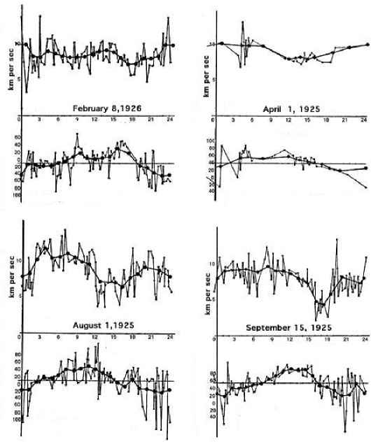
Figure 7: Miller’s results from the 1925-1926 observations of absolute motion showing the projected ‘Michelson’ speed $v_{M}$ in km/s and azimuth angle $\psi$ in degrees plotted against sidereal time in hours. The results are for April, August and September 1925 and February 1926. In most cases the results arise from observations extending over much of each month, i.e not from a single day in each month. Therefore the data points are not strictly in chronological order. The lines joining the data points are merely to make the data points clearer. The smoother line is a running time average computed by Miller. The fluctuations in both $v_{M}$ and $\psi$ appear to be a combination of apparatus effects and genuine physical phenomena caused by turbulence in the gravitational in-flow of space towards the Sun. Each data point arises from analysis of the average of twenty full rotations of the interferometer. The speed data for September is re-plotted in Fig.9 showing the corrected absolute speed.

Note that the above corrected Miller projected absolute speed of approximately $v_{P}=415$km/s is completely consistent with the corrected projected absolute speed of some $330$km/s from the Michelson-Morley experiment, though neither Michelson nor Miller were able to apply this correction. The difference in magnitude is completely explained by Cleveland having a higher latitude than Mt. Wilson, and also by the only two sidereal times of the Michelson-Morley observations. So from his 1925-1926 observations Miller had completely confirmed the true validity of the Michelson-Morley observations and was able to conclude, contrary to their published conclusions, that the 1887 experiment had in fact detected absolute motion. But it was too late. By then the physicists had incorrectly come to believe that absolute motion was inconsistent with various ‘relativistic effects’ that had by then been observed. This was because the Einstein formalism had been ‘derived’ from the assumption that absolute motion was without meaning and so unobservable in principle. Of course the earlier interpretation of relativistic effects by Lorentz had by then lost out to the Einstein interpretation.

(a)

(b)

Figure 8: Expected theoretical variation of both (a) the projected velocity $v_{P}$, and (b) the azimuth $\psi$ during one sidereal day in the months of April, August, September and February, labelled by increasing dash length. These forms assume a cosmic speed of $417$km/s in the direction $(\alpha=4^{hr}54^{m},\delta=-70^{0}33^{\prime})$, and the tangential and in-flows velocities as in (7). These plots show the characteristics of the signature expected in observations of absolute motion.

Figure 9: The absolute projected speeds $v_{P}$, plotted against sidereal time in hours, for September 1925 is re-plotted using the correction $v_{P}=v_{M}/k_{air}$. The data points were obtained from Miller’s original data which was found in 2002. The dip at $\tau\approx 16^{hr}$(ST) is also seen in the New Bedford data, Fig.12, and the DeWitte data, Fig.13. So three different experiments reveal the same absolute motion signature. The fluctuations in $v_{P}$ appear to be a combination of experimental effects and genuine physical phenomena caused by turbulence in the gravitational in-flow of space towards the Sun.

2.5 Gravitational In-flow from the Miller Data

As already noted Miller was led to the conclusion that for reasons unknown the existing theory of the Michelson interferometer did not reveal true values of $v_{P}$, and for this reason he introduced the parameter $k$, with $\overline{k}$ indicating his numerical values. Miller had reasoned that he could determine both ${\bf v}_{cosmic}$ and $\overline{k}$ by observing the interferometer determined $v_{P}$ and $\psi$ over a year because the known orbital velocity of the Earth about the Sun would modulate both of these observables, and by a scaling argument he could determine the absolute velocity of the Solar system. In this manner he finally determined that $|{\bf v}_{cosmic}|=208$ km/s in the direction $(\alpha=4^{hr}54^{m},\delta=-70^{0}33^{\prime})$. However now that the theory of the Michelson interferometer has been revealed an anomaly becomes apparent. Table 3 shows $v=v_{M}/k_{air}$ for each of the four epochs, giving speeds consistent with the revised Michelson-Morley data. However Table 3 also shows that $\overline{k}$ and the speeds $\overline{v}=v_{M}/\overline{k}$ determined by the scaling argument are considerably different. Here the $v_{M}$ values arise after taking account of the projection effect. That $\overline{k}$ is considerably larger than the value of $k_{air}$ indicates that another velocity component has been overlooked. Miller of course only knew of the tangential orbital speed of the Earth, whereas the new physics predicts that as-well there is a quantum-gravity radial in-flow ${\bf v}_{in}$ of the quantum foam. We can re-analyse Miller’s data to extract a first approximation to the speed of this in-flow component. Clearly it is $v_{R}=\sqrt{v_{in}^{2}+v^{2}_{tangent}}$ that sets the scale and not $v_{tangent}$, and because $\overline{k}=v_{M}/v_{tangent}$ and $k_{air}=v_{M}/v_{R}$ are the scaling relations, then

$$v_{in} = v_{tangent}\sqrt{\displaystyle{\frac{v_{R}^{2}}{v_{tangent}^{2}}-1}},$$ (11)

$$= v_{tangent}\sqrt{\displaystyle{\frac{\overline{k}^{2}}{k_{air}^{2}}-1}}.$$

Epoch	$v_{M}$	$\overline{k}$	$v=v_{M}/k_{air}$	$\overline{v}=v_{M}/\overline{k}$	$v=\sqrt{3}\overline{v}$	$v_{in}$
February 8	9.3 km/s	0.048	385.9 km/s	193.8 km/s	335.7 km/s	51.7 km/s
April 1	10.1	0.051	419.1	198.0	342.9	56.0
August 1	11.2	0.053	464.7	211.3	366.0	58.8
September 15	9.6	0.046	398.3	208.7	361.5	48.8

Table 3. The $\overline{k}$ anomaly, $\overline{k}\gg k_{air}=0.0241$, as the gravitational in-flow effect.

Here $v_{M}$ and $\overline{k}$ come from fitting the interferometer data, while $\,v\,$ and $\,\overline{v}\,$ are

computed speeds using the indicated scaling. The average of the in-flow speeds

is $v_{in}=54\pm 5$ km/s, compared to the ‘Newtonian’ in-flow speed of $42$ km/s.

From column 4 we obtain the average $v=417\pm 40$km/s.

Using the $\overline{k}$ values in Table 3 and the value of $k_{air}$ we obtain the $v_{in}$ speeds shown in Table 3, which give an average speed of $54$ km/s, compared to the ‘Newtonian’ in-flow speed of $42$ km/s. Note that the in-flow interpretation of the anomaly predicts that $\overline{k}=(v_{R}/v_{tangent})\,k_{air}=\sqrt{3}\,k_{air}=0.042$. Of course this simple re-scaling of the Miller results is not completely valid because (i) the direction of ${\bf v}_{R}$ is of course different to that of ${\bf v}_{tangent}$, and also not necessarily orthogonal to ${\bf v}_{tangent}$ because of turbulence, and (ii) also because of turbulence we would expect some contribution from the in-flow effect of the Earth itself, namely that it is not always perpendicular to the Earth’s surface, and so would give a contribution to a horizontally operated interferometer.

An analysis that properly searches for the in-flow velocity effect clearly requires a complete re-analysis of the Miller data, and this is now possible and underway at Flinders University as the original data sheets have been found. It should be noted that the direction diametrically opposite $(\alpha=4^{hr}54^{m},\delta=-70^{0}33^{\prime})$, namely $(\alpha=17^{hr},\delta=+68^{\prime})$ was at one stage considered by Miller as being possible. This is because the Michelson interferometer, being a 2nd-order device, has a directional ambiguity which can only be resolved by using the diurnal motion of the Earth. However as Miller did not include the in-flow velocity effect in his analysis it is possible that a re-analysis might give this northerly direction as the direction of absolute motion of the Solar system.

Hence not only did Miller observe absolute motion, as he claimed, but the quality and quantity of his data has also enabled the confirmation of the existence of the gravitational in-flow effect [10, 11]. This is a manifestation of a new theory of gravity and one which relates to quantum gravitational effects via the unification of matter and space developed in previous sections. As well the persistent evidence that this in-flow is turbulent indicates that this theory of gravity involves self-interaction of space itself.

2.6 The Illingworth Experiment: 1927

In 1927 Illingworth [17] performed a Michelson interferometer experiment in which the light beams passed through the gas Helium,

…as it has such a low index of refraction that variations due to temperature changes are reduced to a negligible quantity.

For Helium at STP $n=1.000036$ and so $k^{2}_{He}=0.00007$, which results in an enormous reduction in sensitivity of the interferometer. Nevertheless this experiment gives an excellent opportunity to check the $n$ dependence in (6). Illingworth, not surprisingly, reported no “ether drift to an accuracy of about one kilometer per second”. Múnera [19] re-analysed the Illingworth data to obtain a speed $v_{M}=3.13\pm 1.04$km/s. The correction factor in (6), $1/\sqrt{n_{He}^{2}-1}=118$, is large for Helium and gives $v=368\pm 123$km/s. As shown in Fig.10 the Illingworth observations now agree with those of Michelson-Morley and Miller, though they would certainly be inconsistent without the $n-$dependent correction, as shown in the lower data points (shown at $5\times$ scale).

So the use by Illingworth of Helium gas has turned out have offered a fortuitous opportunity to confirm the validity of the refractive index effect, though because of the insensitivity of this experiment the resulting error range is significantly larger than those of the other interferometer observations. So finally it is seen that the Illingworth experiment detected absolute motion with a speed consistent with all other observations.

Figure 10: Speeds $v$ in km/s determined from various Michelson interferometer experiments (1)-(4) and CMB (5): (1) Michelson-Morley (noon observations) and (2) ($18^{h}$ observations) see Sect.2.3, (3) Illingworth [17], (4) Miller, Mt.Wilson [16], and finally in (5) the speed from observations of the CMB spectrum dipole term [20]. The results (1)-(3) are not corrected for the $\pm 30$km/s of the orbital motion of the Earth about the Sun or for the gravitational in-flow speed, though these correction were made for (4) with the speeds from Table 3. The horizontal line at $v=369$km/s is to aid comparisons with the CMB frame speed data. The Miller direction is different to the CMB direction. Due to the angle between the velocity vector and the plane of interferometer the results (1)-(3) are less than or equal to the true speed, while the result for (4) is the true speed as this projection effect was included in the analysis. These results demonstrate the remarkable consistency between the three interferometer experiments. The Miller speed agrees with the speed from the DeWitte non-interferometer experiment, in Sect.2.8. The lower data, magnified by a factor of 5, are the original speeds $v_{M}$ determined from fringe shifts using (1) with $k=1$. This figure updates the corresponding figure in Ref.[9].

2.7 The New Bedford Experiment: 1963

In 1964 from an absolute motion detector experiment at New Bedford, latitude $42^{0}$N, Jaseja et al [21] reported yet another ‘null result’. In this experiment two He-Ne masers were mounted with axes perpendicular on a rotating table, see Fig.11. Rotation of the table through $90^{0}$ produced repeatable variations in the frequency difference of about $275$kHz, an effect attributed to magnetorestriction in the Invar spacers due to the Earth’s magnetic field. Observations over some six consecutive hours on January 20, 1963 from $6\!\!:\!\!00$ am to $12\!\!:\!\!00$ noon local time did produce a ‘dip’ in the frequency difference of some $3$kHz superimposed on the $275$kHz effect, as shown in Fig.12 in which the local times have been converted to sidereal times. The most noticeable feature is that the dip occurs at approximately $17-18\!\!:\!\!00^{hr}$ sidereal time (or $9-10\!\!:\!\!00$ hrs local time), which agrees with the direction of absolute motion observed by Miller and also by DeWitte (see Sect.2.8). It was most fortunate that this particular time period was chosen as at other times the effect is much smaller, as shown for example in Fig.9 for August or more appropriately for the February data in Fig.7 which shows the minimum at $18\!\!:\!\!00^{hr}$ sidereal time. The local times were chosen by Jaseja et al such that if the only motion was due to the Earth’s orbital speed the maximum frequency difference, on rotation, should have occurred at $12\!\!:\!\!00$hr local time, and the minimum frequency difference at $6\!\!:\!\!00$ hr local time, whereas in fact the minimum frequency difference occurred at $9\!\!:\!\!00$ hr local time.

Figure 11: Schematic diagram for recording the variations in beat frequency between two optical masers: (a) when at absolute rest, (b) when in absolute motion at velocity ${\bf v}$. PM is the photomultiplier detector. The apparatus was rotated back and forth through $90^{0}$.

Figure 12: Frequency difference in kHz between the two masers in the 1963 New Bedford experiment after a $90^{0}$ rotation. The $275$kHz difference is a systematic repeatable apparatus effect, whereas the superimposed ‘dip’ at $17-18\!\!:\!\!00^{hr}$ sidereal time of approximately $3$kHz is a real time dependent frequency difference. The full curve shows the theoretical prediction for the time of the ‘dip’ for this experiment using the Miller direction for ${\bf\hat{v}}$ $(\alpha=4^{hr}54^{m},\delta=-70^{0}33^{\prime})$ with $|{\bf v}|=417$km/s and including the Earth’s orbital velocity and Sun gravitational in-flow velocity effects for January 20, 1963. The absolute scale of this theoretical prediction was not possible to compute as the refractive index of the He-Ne gas mixture was unknown.

As for the Michelson-Morley experiment the analysis of the New Bedford experiment was also bungled. Again this apparatus can only detect the effects of absolute motion if the cancellation between the geometrical effects and Fitzgerald-Lorentz length contraction effects is incomplete as occurs only when the radiation travels in a gas, here the He-Ne gas present in the maser.

This double maser apparatus is essentially equivalent to a Michelson interferometer. Then the resonant frequency $\nu$ of each maser is proportional to the reciprocal of the out-and-back travel time. For maser 1

$$\nu_{1}=m\frac{V^{2}-v^{2}}{2LV\sqrt{1-\displaystyle\frac{v^{2}}{c^{2}}}},$$ (12)

for which a Fitzgerald-Lorentz contraction occurs, while for maser 2

$$\nu_{2}=m\frac{\sqrt{V^{2}-v^{2}}}{2L}.$$ (13)

Here $m$ refers to the mode number of the masers. When the apparatus is rotated the net observed frequency difference is $\delta\nu=2(\nu_{2}-\nu_{1})$, where the factor of ‘2’ arises as the roles of the two masers are reversed after a $90^{0}$ rotation. Putting $V=c/n$ we find for $v<<V$ and with $\nu_{0}$ the at-rest resonant frequency, that

$$\delta\nu=(n^{2}-1)\nu_{0}\frac{v^{2}}{c^{2}}+O(\frac{v^{4}}{c^{4}}).$$ (14)

If we use the Newtonian physics analysis, as in Jaseja et al [21], which neglects both the Fitzgerald-Lorentz contraction and the refractive index effect, then we obtain $\delta\nu=\nu_{0}v^{2}/c^{2}$, that is without the $n^{2}-1$ term, just as for the Newtonian analysis of the Michelson interferometer itself. Of course the very small magnitude of the absolute motion effect, which was approximately 1/1000 that expected assuming only an orbital speed of $v=30$ km/s in the Newtonian analysis, occurs simply because the refractive index of the He-Ne gas is very close to one. Nevertheless given that it is small the sidereal time of the obvious ’dip’ coincides almost exactly with that of the other observations of absolute motion.

The New Bedford experiment was yet another missed opportunity to have revealed the existence of absolute motion. Again the spurious argument was that because the Newtonian physics analysis gave the wrong prediction then Einstein relativity must be correct. But the analysis simply failed to take account of the Fitzgerald-Lorentz contraction, which had been known since the end of the 19^th century, and the refractive index effect which had an even longer history. As well the authors failed to convert their local times to sidereal times and compare the time for the ‘dip’ with Miller’s time.

2.8 The DeWitte Experiment: 1991

The Michelson-Morley, Illingworth, Miller and New Bedford experiments all used Michelson interferometers or its equivalent in gas mode, and all revealed absolute motion. The Michelson interferometer is a 2nd-order device meaning that the time difference between the ‘arms’ is proportional to $(v/c)^{2}$. There is also a factor of $n^{2}-1$ and for gases like air and particularly Helium or Helium-Neon mixes this results in very small time differences and so these experiments were always very difficult. Of course without the gas the Michelson interferometer is incapable of detecting absolute motion, and so there are fundamental limitations to the use of this interferometer in the study of absolute motion and related effects.

Figure 13: Variations in twice the one-way travel time, in ns, for an RF signal to travel 1.5 km through a coaxial cable between Rue du Marais and Rue de la Paille, Brussels. An offset has been used such that the average is zero. The definition of the sign convention for $\Delta t$ used by DeWitte is unclear. The cable has a North-South orientation, and the data is $\pm$ difference of the travel times for NS and SN propagation. The sidereal time for maximum effect of $\sim\!\!17$hr (or $\sim\!\!5$hr) (indicated by vertical lines) agrees with the direction found by Miller and also by Jaseja et al, but because of the ambiguity in the definition of $\Delta t$ the opposite direction would also be consistent with this data. Plot shows data over 3 sidereal days and is plotted against sidereal time. See Fig.14b for theoretical predictions for one sidereal day. The time of the year of the data is not identified. The fluctuations are evidence of turbulence associated with the gravitational in-flow towards the Sun. Adapted from DeWitte [22].

In a remarkable development in 1991 a research project within Belgacom, the Belgium telecommunications company, stumbled across yet another detection of absolute motion, and one which turned out to be 1st-order in $v/c$. The study was undertaken by Roland DeWitte [22]. This organisation had two sets of atomic clocks in two buildings in Brussels separated by 1.5 km and the research project was an investigation of the task of synchronising these two clusters of atomic clocks. To that end 5MHz radiofrequency signals were sent in both directions through two buried coaxial cables linking the two clusters. The atomic clocks were caesium beam atomic clocks, and there were three in each cluster. In that way the stability of the clocks could be established and monitored. One cluster was in a building on Rue du Marais and the second cluster was due south in a building on Rue de la Paille. Digital phase comparators were used to measure changes in times between clocks within the same cluster and also in the propagation times of the RF signals. Time differences between clocks within the same cluster showed a linear phase drift caused by the clocks not having exactly the same frequency together with short term and long term noise. However the long term drift was very linear and reproducible, and that drift could be allowed for in analysing time differences in the propagation times between the clusters.

Changes in propagation times were observed and eventually observations over 178 days were recorded. A sample of the data, plotted against sidereal time for just three days, is shown in Fig.13. DeWitte recognised that the data was evidence of absolute motion but he was unaware of the Miller experiment and did not realise that the Right Ascension for maximum/minimum propagation time agreed almost exactly with Miller’s direction $(\alpha,\delta)=(17.5^{h},65^{0})$. In fact DeWitte expected that the direction of absolute motion should have been in the CMB direction, but that would have given the data a totally different sidereal time signature, namely the times for maximum/minimum would have been shifted by 6 hrs. The declination of the velocity observed in this DeWitte experiment cannot be determined from the data as only three days of data are available. However assuming exactly the same declination as Miller the speed observed by DeWitte appears to be also in excellent agreement with the Miller speed, which in turn is in agreement with that from the Michelson-Morley and Illingworth experiments, as shown in Fig.10.

(a)

(b)

Figure 14: Theoretical predictions for the variations in travel time, in ns, for one sidereal day, in the DeWitte Brussels coaxial cable experiment for ${\bf v}_{cosmic}$ in the direction $(\alpha,\delta)=(17.5^{h},65^{0})$ and with the Miller magnitude of 417 km/s, and including orbital and in-flow effects (but without turbulence). Shown are the results for four days: for the Vernal Equinox, March 21 (shortest dashes), and for 90, 180 and 270 days later (shown with increasing dash length). Figure (a) Shows change in one-way travel time $t_{0}nv_{P}/c$ for signal travelling from N to S. Figure (b) shows $\Delta t$, as defined in (15), with an offset such that the average is zero so as to enable comparison with the data in Fig.13. $\Delta t$ is twice the one-way travel time. For the direction opposite to $(\alpha,\delta)=(17.5^{h},65^{0})$ the same curves arise except that the identification of the months is different and the sign of $\Delta t$ also changes. The sign of $\Delta t$ determines which of the two directions is the actual direction of absolute motion. However the definition of the sign convention for $\Delta t$ used by DeWitte is unclear.

Being 1st-order in $v/c$ the Belgacom experiment is easily analysed to sufficient accuracy by ignoring relativistic effects, which are 2nd-order in $v/c$. Let the projection of the absolute velocity vector ${\bf v}$ onto the direction of the coaxial cable be $v_{P}$ as before. Then the phase comparators reveal the difference between the propagation times in NS and SN directions. First consider the analysis with no Fresnel drag effect,

$$\Delta t = \frac{L}{\displaystyle{\frac{c}{n}}-v_{P}}-\frac{L}{\displaystyle{\frac{c}{n}}+v_{P}},$$ (15)

$$= 2\frac{L}{c/n}n\frac{v_{P}}{c}+O(\frac{v_{P}^{2}}{c^{2}})\approx 2t_{0}n\frac{v_{P}}{c}.$$

Here $L=1.5$ km is the length of the coaxial cable, $n=1.5$ is the refractive index of the insulator within the coaxial cable, so that the speed of the RF signals is approximately $c/n=200,000$km/s, and so $t_{0}=nL/c=7.5\times 10^{-6}$ sec is the one-way RF travel time when $v_{P}=0$. Then, for example, a value of $v_{P}=400$km/s would give $\Delta t=30$ns. Because Brussels has a latitude of $51^{0}$ N then for the Miller direction the projection effect is such that $v_{P}$ almost varies from zero to a maximum value of $|{\bf v}|$. The DeWitte data in Fig.13 shows $\Delta t$ plotted with a false zero, but shows a variation of some 28 ns. So the DeWitte data is in excellent agreement with the Miller’s data. The Miller experiment has thus been confirmed by a non-interferometer experiment if we ignore a Fresnel drag.

But if we include a Fresnel drag effect then the change in travel time $\Delta t_{F}$ becomes

$$\Delta t_{F} = \frac{L}{\displaystyle{\frac{c}{n}}+bv_{P}-v_{P}}-\frac{L}{\displaystyle{\frac{c}{n}}-bv_{P}+v_{P}},$$ (16)

$$= 2\frac{L}{c}\frac{v_{P}}{c}+O(\frac{v_{P}^{2}}{c^{2}}),$$

$$= \frac{1}{n^{2}}\Delta t,$$

where $b=1-1/n^{2}$ is the Fresnel drag coefficient. Then $\Delta t_{F}$ is smaller than $\Delta t$ by a factor of $n^{2}=1.5^{2}=2.25$, and so a speed of $v_{P}=2.25\times 400=900$ km/s would be required to produce a $\Delta t_{F}=30$ ns. This speed is inconsistent with the results from gas-mode interferometer experiments, and also inconsistent with the data from the Torr-Kolen gas-mode coaxial cable experiment, Sect.2.9. This raises the question as to whether the Fresnel effect is present in transparent solids, and indeed whether it has ever been studied? As well we are assuming the conventional eletromagnetic theory for the RF fields in the coaxial cable. An experiment to investigate this is underway at Flinders university [1].

The actual days of the data in Fig.13 are not revealed in Ref.[22] so a detailed analysis of the DeWitte data is not possible. Nevertheless theoretical predictions for various days in a year are shown in Fig.14 using the Miller speed of $v_{cosmic}=417$ km/s (from Table 3) and where the diurnal effects of the Earth’s orbital velocity and the gravitational in-flow cause the range of variation of $\Delta t$ and sidereal time of maximum effect to vary throughout the year. The predictions give $\Delta t=30\pm 4$ ns over a year compared to the DeWitte value of 28 ns in Fig.13. If all of DeWitte’s 178 days of data were available then a detailed analysis would be possible.

Ref.[22] does however reveal the sidereal time of the cross-over time, that is a ‘zero’ time in Fig.13, for all 178 days of data. This is plotted in Fig.15 and demonstrates that the time variations are correlated with sidereal time and not local solar time. A least squares best fit of a linear relation to that data gives that the cross-over time is retarded, on average, by 3.92 minutes per solar day. This is to be compared with the fact that a sidereal day is 3.93 minutes shorter than a solar day. So the effect is certainly cosmological and not associated with any daily thermal effects, which in any case would be very small as the cable is buried. Miller had also compared his data against sidereal time and established the same property, namely that up to small diurnal effects identifiable with the Earth’s orbital motion, features in the data tracked sidereal time and not solar time; see Ref.[16] for a detailed analysis.

Figure 15: Plot of the negative of the drift of the cross-over time between minimum and maximum travel-time variation each day (at $\sim 10^{h}\pm 1^{h}$ ST) versus local solar time for some 180 days. The straight line plot is the least squares fit to the experimental data, giving an average slope of 3.92 minutes/day. The time difference between a sidereal day and a solar day is 3.93 minutes/day. This demonstrates that the effect is related to sidereal time and not local solar time. The actual days of the year are not identified in Ref.[22]. Adapted from DeWitte [22].

The DeWitte data is also capable of resolving the question of the absolute direction of motion found by Miller. Is the direction $(\alpha,\delta)=(17.5^{h},65^{0})$ or the opposite direction? Being a 2nd-order Michelson interferometer experiment Miller had to rely on the Earth’s diurnal effects in order to resolve this ambiguity, but his analysis of course did not take account of the gravitational in-flow effect, and so until a re-analysis of his data his preferred choice of direction must remain to be confirmed. The DeWitte experiment could easily resolve this ambiguity by simply noting the sign of $\Delta t$. Unfortunately it is unclear in Ref.[22] as to how the sign in Fig.13 is actually defined, and DeWitte does not report a direction expecting, as he did, that the direction should have been the same as the CMB direction.

The DeWitte observations were truly remarkable considering that initially they were serendipitous. They demonstrated yet again that the Einstein postulates were in contradiction with experiment. To my knowledge no physics journal has published a report of the DeWitte experiment.

That the DeWitte experiment is not a gas-mode Michelson interferometer experiment is very significant. The value of the speed of absolute motion revealed by the DeWitte experiment of some 400 km/s is in agreement with the speeds revealed by the new analysis of various Michelson interferometer data which uses the recently discovered refractive index effect, see Fig.10. Not only was this effect confirmed by comparing results for different gases, but the re-scaling of the older $v_{M}$ speeds to $v=v_{M}/\sqrt{n^{2}-1}$ speeds resulting from this effect are now confirmed. A new and much simpler 1st-order experiment is discussed in [1] which avoids the use of atomic clocks.

2.9 The Torr-Kolen Experiment: 1981

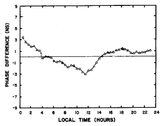
Figure 16: Upper figure is data from the 1981 Torr-Kolen experiment at Logan, Utah [23]. The data shows variations in travel times (ns), for local times, of an RF signal travelling through 500m of coaxial cable orientated in an E-W direction. Actual days are not indicated but the experiment was done during February-June 1981. Results are for a typical day. For the 1st of February the local time of $12\!\!:\!\!00$ corresponds to $13\!\!:\!\!00$ sidereal time. The predictions are for March (shortest dashes) and June, for a cosmic speed of $417$ km/s in the direction $(\alpha,\delta)=(17.5^{h},65^{0})$, and including orbital and in-flow velocities but without theoretical turbulence.

A coaxial cable experiment similar to but before the DeWitte experiment was performed at the Utah University in 1981 by Torr and Kolen [23]. This involved two rubidium vapor clocks placed approximately 500m apart with a 5 MHz sinewave RF signal propagating between the clocks via a nitrogen filled coaxial cable maintained at a constant pressure of $\sim$2 psi. This means that the Fresnel drag effect is not important in this experiment. Unfortunately the cable was orientated in an East-West direction which is not a favourable orientation for observing absolute motion in the Miller direction, unlike the Brussels North-South cable orientation. There is no reference to Miller’s result in the Torr and Kolen paper, otherwise they would presumably not have used this orientation. Nevertheless there is a projection of the absolute motion velocity onto the East-West cable and Torr and Kolen did observe an effect in that, while the round speed time remained constant within 0.0001%c, typical variations in the one-way travel time were observed, as shown in Fig.16 by the triangle data points. The theoretical predictions for the Torr-Kolen experiment for a cosmic speed of $417$ km/s in the direction $(\alpha,\delta)=(17.5^{h},65^{0})$, and including orbital and in-flow velocities, are shown in Fig.16. As well the maximum effect occurred, typically, at the predicted times. So the results of this experiment are also in remarkable agreement with the Miller direction, and the speed of 417 km/s which of course only arises after re-scaling the Miller speeds for the effects of the gravitational in-flow. As well Torr and Kolen reported fluctuations in both the magnitude and time of the maximum variations in travel time just as DeWitte observed some 10 years later. Again we argue that these fluctuations are evidence of genuine turbulence in the in-flow as discussed in Sect.2.11. So the Torr-Kolen experiment again shows strong evidence for the new theory of gravity, and which is over and above its confirmation of the various observations of absolute motion.

2.10 Galactic In-flow and the CMB Frame

Absolute motion (AM) of the Solar system has been observed in the direction $(\alpha=17.5^{h},\delta=65^{0})$, up to an overall sign to be sorted out, with a speed of $417\pm 40$ km/s. This is the velocity after removing the contribution of the Earth’s orbital speed and the Sun in-flow effect. It is significant that this velocity is different to that associated with the Cosmic Microwave Background (CMB) relative to which the Solar system has a speed of $369$ km/s in the direction $(\alpha=11.20^{h},\delta=-7.22^{0})$, see [20]. This CMB velocity is obtained by finding the preferred frame in which this thermalised $3^{0}$K radiation is isotropic, that is by removing the dipole component. The CMB velocity is a measure of the motion of the Solar system relative to the universe as a whole, or aleast a shell of the universe some 15Gyrs away, and indeed the near uniformity of that radiation in all directions demonstrates that we may meaningfully refer to the spatial structure of the universe. The concept here is that at the time of decoupling of this radiation from matter that matter was on the whole, apart from small observable fluctuations, at rest with respect to the quantum-foam system that is space. So the CMB velocity is the motion of the Solar system with respect to space universally, but not necessarily with respect to the local space. Contributions to this velocity would arise from the orbital motion of the Solar system within the Milky Way galaxy, which has a speed of some 250 km/s, and contributions from the motion of the Milky Way within the local cluster, and so on to perhaps larger clusters.

On the other hand the AM velocity is a vector sum of this universal CMB velocity and the net velocity associated with the local gravitational in-flows into the Milky Way and the local cluster. If the CMB velocity had been identical to the AM velocity then the in-flow interpretation of gravity would have been proven wrong. We therefore have three pieces of experimental evidence for this interpretation (i) the refractive index anomaly discussed previously in connection with the Miller data, (ii) the turbulence seen in all detections of absolute motion, and now (iii) that the AM velocity is different in both magnitude and direction from that of the CMB velocity, and that this velocity does not display the turbulence seen in the AM velocity.

That the AM and CMB velocities are different amounts to the discovery of the resolution to the ‘dark matter’ conjecture. Rather than the galactic velocity anomalies being caused by such undiscovered ‘dark matter’ we see that the in-flow into non spherical galaxies, such as the spiral Milky Way, will be non Newtonian [1]. As well it will be interesting to determine, at least theoretically, the scale of turbulence expected in galactic systems, particularly as the magnitude of the turbulence seen in the AM velocity is somewhat larger than might be expected from the Sun in-flow alone. Any theory for the turbulence effect will certainly be checkable within the Solar system as the time scale of this is suitable for detailed observation.

It is also clear that the time of obervers at rest with respect to the CMB frame is absolute or universal time. This interpretation of the CMB frame has of course always been rejected by supporters of the SR/GR formalism. As for space we note that it has a differential structure, in that different regions are in relative motion. This is caused by the gravitational in-flow effect locally, and as well by the growth of the universe.

2.11 In-Flow Turbulence and Gravitational Waves

Figure 17: Speed fluctuations determined from Fig.13 by subtracting a least squares best fit of the forms shown in Fig.14b. A 1ns variation in travel time corresponds approximately to a speed variation of 27km/s. The larger speed fluctuations actually arise from a fluctuation in the cross-over time, that is, a fluctuation in the direction of the velocity. This plot implies that the velocity flow-field is turbulent. The scale of this turbulence is comparable to that evident in the Miller data, as shown in Fig.7 and Fig.9.

The velocity flow-field equation [1] is expected to have solutions possessing turbulence, that is, random fluctuations in both the magnitude and direction of the gravitational in-flow component of the velocity flow-field. Indeed all the Michelson interferometer experiments showed evidence of such turbulence. The first clear evidence was from the Miller experiment, as shown in Fig.7 and Fig.9. Miller offered no explanation for these fluctuations but in his analysis of that data he did running time averages, as shown by the smoother curves in Fig.7. Miller may have in fact have simply interpreted these fluctuations as purely instrumental effects. While some of these fluctuations may be partially caused by weather related temperature and pressure variations, the bulk of the fluctuations appear to be larger than expected from that cause alone. Even the original Michelson-Morley data in Fig.5 shows variations in the velocity field and supports this interpretation. However it is significant that the non-interferometer DeWitte data also shows evidence of turbulence in both the magnitude and direction of the velocity flow field, as shown in Fig.17. Just as the DeWitte data agrees with the Miller data for speeds and directions the magnitude fluctuations, shown in Fig.17, are very similar in absolute magnitude to, for example, the speed turbulence shown in Fig.9.

It therefore becomes clear that there is strong evidence for these fluctuations being evidence of physical turbulence in the flow field. The magnitude of this turbulence appears to be somewhat larger than that which would be caused by the in-flow of quantum foam towards the Sun, and indeed following on from Sect.2.10 some of this turbulence may be associated with galactic in-flow into the Milky Way. This in-flow turbulence is a form of gravitational wave and the ability of gas-mode Michelson interferometers to detect absolute motion means that experimental evidence of such a wave phenomena has been available for a considerable period of time, but suppressed along with the detection of absolute motion itself. Of course flow equations do not exhibit those gravitational waves of the form that have been predicted to exist based on the Einstein equations, and which are supposed to propagate at the speed of light. All this means that gravitational wave phenomena is very easy to detect and amounts to new physics that can be studied in much detail, particularly using the new 1st-order interferometer discussed in [1].

2.12 Vacuum Michelson Interferometers

Over the years vacuum-mode Michelson interferometer experiments have become increasing popular, although the motivation for such experiments appears to be increasingly unclear. The first vacuum interferometer experiment was by Joos [24] in 1930 and gave $v_{M}<1$km/s. This result is consistent with a null effect as predicted by both the quantum-foam physics and the Einstein physics. Only Newtonian physics is disproved by such experiments. These vacuum interferometer experiments do give null results, with increasing confidence level, as for example in Refs.[25, 26, 27, 28], but they only check that the Lorentz contraction effect completely cancels the geometrical path-length effect in vacuum experiments, and this is common to both theories. So they are unable to distinguish the new physics from the Einstein physics. Nevertheless recent works [27, 28] continue to claim that the experiment had been motivated by the desire to look for evidence of absolute motion, despite effects of absolute motion having been discovered as long ago as 1887. The ‘null results’ are always reported as proof of the Einstein formalism. Of course all the vacuum experiments can do is check the Lorentz contraction effect, and this in itself is valuable. Unfortunately the analysis of the data from such experiments is always by means of the Robertson [29] and Mansouri and Sexl formalism [30], which purports to be a generalisation of the Lorentz transformation if there is a preferred frame. However in [1] we have already noted that absolute motion effects, that is the existence of a preferred frame, are consistent with the usual Lorentz transformation, based as it is on the restricted Einstein measurement protocol. A preferred frame is revealed by gas-mode Michelson interferometer experiments, and then the refractive index of the gas plays a critical role in interpreting the data. The Robertson and Mansouri-Sexl formalism contains no contextual aspects such as a refractive index effect and is thus totally inappropriate to the analysis of so called ‘preferred frame’ experiments.

It is a curious feature of the history of Michelson interferometer experiments that it went unnoticed that the results fell into two distinct classes, namely vacuum and gas-mode, with recurring non-null results from gas-mode interferometers.

2.13 Solid-State Michelson Interferometers

The gas-mode Michelson interferometer has its sensitivity to absolute motion effects greatly reduced by the refractive index effect, namely the $k^{2}=n^{2}-1$ factor in (1), and for gases with $n$ only slightly greater than one this factor has caused much confusion over the last 115 years. So it would be expected that passing the light beams through a transparent solid with $n\approx 1.5$ rather than through a gas would greatly increase the sensitivity. Such an Michelson interferometer experiment was performed by Shamir and Fox [31] in Haifa in 1969. This interferometer used light from a He-Ne laser and used perspex rods with $L=0.26$m. The experiment was interpreted in terms of the supposed Fresnel drag effect, which has a drag coefficient given by $b=1-1/n^{2}$. The light passing through the solid was supposed to be ‘dragged’ along in the direction of motion of the solid with a velocity $\Delta{\bf V}=b{\bf v}$ additional to the usual $c/n$ speed. As well the Michelson geometrical path difference and the Lorentz contraction effects were incorporated into the analysis. The outcome was that no fringe shifts were seen on rotation of the interferometer, and Shamir and Fox concluded that this negative result “enhances the experimental basis of special relativity”.

The Shamir-Fox experiment was unknown to us at Flinders university when in 2002 several meters of optical fibre were used in a Michelson interferometer experiment which also used a He-Ne laser light source. Again because of the $n^{2}-1$ factor, and even ignoring the Fresnel drag effect, one would have expected large fringe shifts on rotation of the interferometer, but none were observed. As well in a repeat of the experiment single-mode optical fibres were also used and again with no rotation effect seen. So this experiment is consistent with the Shamir-Fox experiment. Re-doing the analysis by including the supposed Fresnel drag effect, as Shamir and Fox did, makes no material difference to the expected outcome. In combination with the non-null results from the gas-mode interferometer experiments along with the non-interferometer experiment of DeWitte it is clear that transparent solids behave differently to a gas when undergoing absolute motion through the quantum foam. Indeed this in itself is a discovery of a new phenomena.

The most likely explanation is that the physical Fitzgerald-Lorentz contraction effect has a anisotropic effect on the refractive index of the transparent solid, and this is such as to cause a cancellation of any differences in travel time between the two arms on rotation of the interferometer. In this sense a transparent solid medium shares this outcome with the vacuum itself.

2.14 Absolute Motion and Quantum Gravity

Absolute rotational motion had been recognised as a meaningful and obervable phenomena from the very beginning of physics. Newton had used his rotating bucket experiment to illustrate the reality of absolute rotational motion, and later Foucault and Sagnac provided further experimental proof. But for absolute linear motion the history would turm out to be completely different. It was generally thought that absolute linear motion was undetectable, at least until Maxwell’s electromagnetic theory appeared to require it. In perhaps the most bizarre sequence of events in modern science it turns out that absolute linear motion has been apparent within experimental data for over 100 years. It was missed in the first experiment designed to detect it and from then on for a variety of sociological reasons it became a concept rejected by physicists and banned from their journals despite continuing new experimental evidence. Those who pursued the scientific evidence were treated with scorn and ridicule. Even worse was the impasse that this obstruction of the scientific process resulted in, namely the halting of nearly all progress in furthering our understanding of the phenomena of gravity. For it is clear from all the experiments that were capable of detecting absolute motion that there is present in that data evidence of turbulence within the velocity field. Both the in-flow itself and the turbulence are manifestations at a classical level of what is essentially quantum gravity processes.

Process Physics has given a unification of explanation and description of physical phenomena based upon the limitations of formal syntactical systems which had nevertheless achieved a remarkable encapsulation of many phenomena, albeit in a disjointed and confused manner, and with a dysfunctional ontology attached for good measure. As argued in early sections space is a quantum system continually classicalised by on-going non-local collapse processes. The emergent phenomena is foundational to existence and experientialism. Gravity in this system is caused by differences in the rate of processing of the cellular information within the network which we experience as space, and consequentially there is a differential flow of information which can be affected by the presence of matter or even by space itself. Of course the motion of matter including photons with respect to that spatial information content is detectable because it affects the geometrical and chronological attributes of that matter, and the experimental evidence for this has been exhaustively discussed in this section. What has become very clear is that the phenomena of gravity is only understandable once we have this unification of the quantum phenomena of matter and the quantum phenomena of space itself. In Process Physics the difference between matter and space is subtle. It comes down to the difference between informational patterns that are topologically preserved and those information patterns that are not. One outcome of this unification is that as a consequence of having a quantum phenomena of space itself we obtain an informational explanation for gravity, and which at a suitable level has an emergent quantum description. In this sense we have an emergent quantum theory of gravity. Of course no such quantum description of gravity is derivable from quantising Einsteinian gravity itself. This follows on two counts, one is that the Einstein gravity formalism fails on several levels, as discussed previously, and second that quantisation has no validity as a means of uncovering deeper physics. Most surprising of all is that having uncovered the logical necessity for gravitational phenomena it also appears that even the seemingly well-founded Newtonian account of gravity has major failings. The denial of this possibility has resulted in an unproductive search for dark matter. Indeed like dark matter and spacetime much of present day physics has all the hallmarks of another episode of Ptolemy’s epicycles, namely concepts that appear to be well founded but in the end turn out to be illusions, and ones that have acquired the status of dogma.

If the Michelson-Morley experiment had been properly analysed and the phenomena revealed by the data exposed, and this would have required in 1887 that Newtonian physics be altered, then as well as the subsequent path of physics being very different, physicists would almost certainly have discovered both the gravitational in-flow effect and associated turbulence.

It is clear then that observation and measurement of absolute motion leads directly to a changed paradigm regarding the nature and manifestations of gravitational phenomena, and that the new 1st-order interferometer described in [1] will provide an extremely simple device to uncover aspects of gravity previously denied by current physics. There are two aspects of such an experimental program. One is the characterisation of the turbulence and its linking to the new non-linear term in the velocity field theory. This is a top down program. The second aspect is a bottom-up approach where the form of the velocity field theory, or its modification, is derived from the deeper informational process physics. This is essentially the quantum gravity route. The turbulence is of course essentially a gravitational wave phenomena and networks of 1st-order interferometers will permit spatial and time series analysis. There are a number of other gravitational anomalies which may also now be studied using such an interferometer network, and so much new physics can be expected to be uncovered.

3 Conclusions

We have shown here that six experiments so far have clearly revealed experimental evidence of absolute motion. As well these are all consistent with respect to the direction and speed of that motion. This clearly refutes the fundamental postulates of the Einstein reinterpretation of the relativitsic effects that had been developed by Lorentz and others. Indeed these experiments are consistent with the Lorentzian relativity in which reality displays both absolute motion effects and relativistic effects. As discussed in detail in [1] it is absolute motion that actually causes these relativistic effects. As well these absolute motion experiments have given experimental support for a new theory of gravity. These developments are discussed more extensively in [1].

4 References

References

- [1] R.T. Cahill, Process Physics: From Information Theory to Quantum Space and Matter, available at http://www.scieng.flinders.edu.au/cpes/people/cahill_r/processphysics.html
- [2] R.T. Cahill, Gravity as Quantum Foam In-Flow.
- [3] R.T. Cahill, Process Physics: Inertia, Gravity and the Quantum, Gen. Rel. and Grav. 34, 1637-1656(2002).
-
[4]
R.T. Cahill, Process Physics: From Quantum Foam to General Relativity,
gr-qc/0203015. -
[5]
R.T. Cahill and C.M. Klinger, Bootstrap Universe from Self-Referential Noise,
gr-qc/9708013. - [6] R.T. Cahill and C.M. Klinger, Self-Referential Noise and the Synthesis of Three-Dimensional Space, Gen. Rel. and Grav. 32(3), 529(2000); gr-qc/9812083.
-
[7]
R.T. Cahill and C.M. Klinger, Self-Referential Noise
as a Fundamental Aspect of Reality,
Proc. 2nd Int. Conf. on Unsolved Problems of Noise and Fluctuations
(UPoN’99), Eds. D. Abbott and L. Kish, Adelaide, Australia, 11-15th July
1999, Vol. 511, p. 43 (American Institute of Physics, New York, 2000);
gr-qc/9905082. - [8] R.T. Cahill, C.M. Klinger, and K. Kitto, Process Physics: Modelling Reality as Self-Organising Information, The Physicist 37(6), 191(2000); gr-qc/0009023.
- [9] R.T. Cahill and K. Kitto, Michelson-Morley Experiments Revisited and the Cosmic Background Radiation Preferred Frame, Apeiron 10, No.2. 104-117(2003); physics/0205070.
-
[10]
R.T. Cahill, Analysis of Data from a Quantum Gravity Experiment,
physics/0207010. - [11] R.T. Cahill, Absolute Motion and Quantum Gravity, physics/0209013.
- [12] K. Kitto, Dynamical Hierarchies in Fundamental Physics, p55, in Workshop Proceedings of the 8th International Conference on the Simulation and Synthesis of Living Systems (ALife VIII), E. Bilotta et al., Eds. (Univ. New South Wales, Australia, 2002).
- [13] M. Chown, Random Reality, New Scientist, Feb 26, 165, No 2227, 24-28(2000).
- [14] A.A. Michelson, Amer. J. Sci. S. 3 22, 120-129(1881).
-
[15]
A.A. Michelson and E.W. Morley, Philos. Mag. S.5, 24, No. 151,
449-463(1887), (available at
http://www.scieng.flinders.edu.au/cpes/people/cahill_r/processphysics.html) -
[16]
D.C. Miller, The Ether-Drift Experiment and the Determination of the
Absolute Motion of the Earth, Rev. Mod. Phys. 5, 203-242(1933), (available at
http://www.scieng.flinders.edu.au/cpes/people/cahill_r/processphysics.html) - [17] K.K. Illingworth, Phys. Rev. 30, 692-696(1927).
- [18] W.M. Hicks, Phil. Mag, [6], 3, 256, 555(1902); 9, 555(1902).
- [19] H.A. Munéra, Aperion 5, No.1-2, 37-54(1998).
- [20] C. Lineweaver et al., Astrophysics J. 470, 38(1996).
- [21] T.S. Jaseja, A. Javan, J. Murray and C.H. Townes, Test of Special Relativity or Isotropy of Space by Use of Infrared Masers, Phys. Rev. A 133, 1221(1964).
- [22] R. DeWitte, http://www.ping.be/~pin30390/.
- [23] D.G. Torr and P. Kolen, Precision Measurements and Fundamental Constants, B.N. Taylor and W.D. Phillips, Eds. Natl. Bur. Stand.(U.S.), Spec. Publ. 617, 675(1984).
- [24] G. Joos, Ann. d. Physik [5], 7, 385(1930).
- [25] H.P Kennedy and E.M. Thorndike, Rev. Mod. Phys. 42 400(1932).
- [26] A. Brillet and J.L. Hall, Phys. Rev. Lett. 42, No.9, 549-552(1979).
- [27] C. Braxmaier, H. Müller, O. Pradl, J. Mlynek, A. Peters and S. Schiller, Phys. Rev. Lett. 88, 010401(2002).
- [28] J.A. Lipa, J.A. Nissen, S. Wang, D.A. Striker and D. Avaloff, Phys. Rev. Lett. 90, 060403-1(2003).
- [29] H.P. Robertson, Rev. Mod. Phys., 21, 378(1949).
- [30] R.M. Mansouri and R.U. Sexl, J. Gen. Rel. Grav., 8, 497(1977), 8, 515(1977), 8, 809(1977).
- [31] J. Shamir and R. Fox, Il Nuovo Cimenta, LXII B N.2, 258(1969).