Fusion process of Lennard-Jones clusters: global minima and magic numbers formation.

Abstract

We present a new theoretical framework for modelling the fusion process of Lennard-Jones (LJ) clusters. Starting from the initial tetrahedral cluster configuration, adding new atoms to the system and absorbing its energy at each step, we find cluster growing paths up to the cluster sizes of up to 150 atoms. We demonstrate that in this way all known global minima structures of the LJ-clusters can be found. Our method provides an efficient tool for the calculation and analysis of atomic cluster structure. With its use we justify the magic number sequence for the clusters of noble gas atoms and compare it with experimental observations. We report the striking correspondence of the peaks in the dependence on cluster size of the second derivative of the binding energy per atom calculated for the chain of LJ-clusters based on the icosahedral symmetry with the peaks in the abundance mass spectra experimentally measured for the clusters of noble gas atoms. Our method serves an efficient alternative to the global optimization techniques based on the Monte-Carlo simulations and it can be applied for the solution of a broad variety of problems in which atomic cluster structure is important.

I Introduction

It is well known that the sequence of cluster magic numbers carries essential information about the electronic and ionic structure of the cluster LesHouches . Understanding of the cluster magic numbers is often equivalent or nearly equivalent to the understanding of cluster electronic and ionic structure. A good example of this kind is the observation of the magic numbers in the mass spectrum of sodium clusters Knight84 . In this case, the magic numbers were explained by the delocalized electron shell closings (see MetCl99 and references therein). Another example is the discovery of fullerenes, and, in particular, the $C_{60}$ molecule Kroto85 , which was made by means of the carbon clusters mass spectroscopy.

The formation of a sequence of cluster magic numbers should be closely connected to the mechanisms of cluster fusion. It is natural to expect that one can explain the magic number sequence and find the most stable cluster isomers by modeling mechanisms of cluster assembly and growth. On the other hand, these mechanisms are of interest on their own, and the correct sequence of the magic numbers found in such a simulation can be considered as a proof of the validity of the cluster formation model.

The problem of magic numbers is closely connected to the problem of searching for global minima on the cluster multidimensional potential energy surface. The number of local minima on the potential energy surface increases exponentially with the growth cluster size and is estimated to be of the order of $10^{43}$ for $N=100$ LesHouches . Thus, searching for global minima becomes increasingly difficult problem for large clusters. There are different algorithms and methods of the global minimization, which have been employed for the global minimization of atomic cluster systems.

One of the most widely used global optimization methods calls the simulated annealing Kirkpatrick ; Wille ; Ma93 ; Ma94 ; Tsoo ; Laaarhoven . This method is an extension of metropolis Monte Carlo techniques Kalos . In the simulated annealing one starts calculation from a high energy state of the system and then cools the system down by decreasing its kinetic energy. In standard application, the system is annealed using molecular dynamics or Monte-Carlo based methods, but also more sophisticated variants of this algorithm are used, such as gaussian density annealing and analogues Ma93 ; Ma94 ; Tsoo .

A related method is quantum tunnelling Finnila ; Amara ; Sylvain . This method attempts to reduce the effects of barriers on the potential energy surface. This is done by allowing the system to behave quantum mechanically, leading to the possibility of tunnelling. However, the computational expense of this method grows exponentially with increasing the number of atoms in the system, what makes this method applicable for relatively small clusters Maranas92 ; Maranas94 .

Another class of global optimization methods is based on smoothing the potential energy surface Stillinger ; Piela ; Pillardy . Within the framework of this method, a transformation is applied to the potential energy surface in order to decrease the number of high lying local minima. The global minimum of the smoothed potential energy surface, which is found by steepest descent energy minimization method, or by Monte-Carlo search, is then mapped back to the original surface.

Another successful method of global optimization is the basin-hopping algorithm LesHouches ; Wales ; Leary . This method involves a potential energy transformation, which does not change neither the global minimum, nor the relative energies of local minima as it is usually done in the potential energy surface smoothing methods. In this method, the potential energy surface in any point of the configuration space is assigned to that of the local minimum obtained by the given geometry optimization method and the potential energy surface is mapped onto a collection of interpenetrating staircases with basins corresponding to the set of configurations which lead to a given minimum after optimization.

Successful global optimization results for LJ clusters reported to date were obtained with the use of genetic algorithms Goldberg ; Niesse ; Gregurick ; Deaven ; Romero . These methods are based on the idea that the population of clusters evolves to low energy by mutation and mating of structures with low potential energy. There are different versions of genetic algorithm (see papers cited above). One of them is seeding algorithm, or seed growth method Niesse ; Gregurick . In this method it is assumed that the most stable cluster of $N$ particles can be obtained from the most stable cluster of $N-1$ particle by a random addition of one particle near the boundary of the cluster and then by optimizing the structure with a given optimization method. Genetic algorithms and other methods related to them are based on stochastic minimization technique, and require no quantum calculation or much information about the potential energy surface, as the previously mentioned algorithms.

The new algorithm GrowProcPRL which we describe in detail in this work for the first time is based on the dynamic searching for the most stable cluster isomers in the cluster fusion process. We call this algorithm as the cluster fusion algorithm (CFA). Our calculations demonstrate that the CFA can be considered as an efficient alternative to the known techniques of the cluster global minimization. The big advantage of the CFA consists in the fact that it allows to study not just the optimized cluster geometries, but also their formation mechanisms.

In the present work we approach the formulated problem in a simple, but general, form. In our simplest scenario, we assume that atoms in a cluster are bound by LJ potential and the cluster fusion takes place atom by atom. At each step of the fusion process all atoms in the system are allowed to move, while the energy of the system is decreased. The motion of the atoms is stopped when the energy minimum is reached. The geometries and energies of all cluster isomers found in this way are stored and analyzed. On the first glance, this method is somewhat similar to the genetic algorithms and to the seed growth method, in particular. However, the principle difference between the CFA and the genetic algorithms consists in the fact that in CFA the new atoms are fused to the system not randomly, but to certain specific points in the system, like the cluster centre of mass, the centres of mass of the cluster faces or some specific points in the vicinity of the cluster surface (see section II for detail). Such an approach, allows one to model various physical situations and scenarios of the cluster fusion process, which are beyond the scope of the stochastic seed-growth method. Thus, with the use of the CFA, we have determined the fusion paths for all known global energy minimum LJ cluster configurations in the size range up to $N\leq 150$. We have also determined the fusion paths for the chains of clusters based on the icosahedral, octahedral, decahedral and tetrahedral symmetries. We report the striking correspondence of the peaks in the dependence on cluster size of the second derivative of the binding energy per atom calculated for the chain of LJ clusters based on the icosahedral symmetry with the peaks in the abundance mass spectra experimentally measured for the clusters of noble gas atoms Echt81 ; Haberland94 ; Harris84 .

Our paper is organized as follows. In section II, we describe theoretical model for the cluster fusion process and the CFA. In section III, we present and discuss the results of computer simulations based on the CFA. In section IV, we draw a conclusion to this paper. In Appendix A, we provide additional details of the numerical algorithms developed in our work.

II Theoretical model for cluster fusion process

A group of atoms bound together by interatomic forces is called an atomic cluster (AC). There is no qualitative distinction between small clusters and molecules. However, as the number of atoms in the system increases, ACs acquire more and more specific properties making them unique physical objects different from both single molecules and from the solid state.

Each stable cluster configuration corresponds to a minimum on the multidimensional potential energy surface of the system. The number of local minima on the potential energy surface increases very rapidly with the growth cluster size. Thus, searching for the most stable cluster configurations possessing the absolute energy minimum, the so-called global energy minimum structures, becomes increasingly difficult problem for large clusters.

Searching for such global energy minimum cluster structures is one of the focuses of our paper. This problem by itself is not new as it is clear from introduction. However, in our work we approach this problem at a new perspective and investigate not just the global energy minimum cluster structure by its own, but rather the formation of such structures in the cluster fusion process.

From the physical point of view, it is natural to expect that one can find the most stable cluster isomers by modeling the mechanisms of cluster assembly and growth, i.e. the cluster fusion process GrowProcPRL . This idea is based on the fact that in nature, or in laboratory, the most stable clusters are often obtained namely in the fusion process. This idea is general and is applicable to different types of clusters.

In this work we consider ACs formed by atoms interacting with each other via the pairing force. The interaction potential between two atoms in the cluster can, in principle, be arbitrary. For concrete computations, we use the Lennard-Jones (LJ) potential,

$$U(r)=4\varepsilon\left(\left(\frac{\sigma}{r}\right)^{12}-\left(\frac{\sigma}{r}\right)^{6}\right),$$ (1)

where $r$ is the interatomic distance, $\varepsilon$ is the depth of the potential well ($\varepsilon>0$), $2^{1/6}\sigma$ is the pair bonding length. The constants in the potential allow one to model various types of clusters for which LJ paring force approximation is reasonable. The most natural systems of this kind are the clusters consisting of noble gas atoms Ne, Ar, Kr, Xe formed by van der Waals forces. The constants of the LJ potential appropriate for the noble gas atoms one can find in RS . Thus, for Ne, Ar, Kr, Xe, $\varepsilon=3.6$, $12.3$, $17.2$, $24.3$ meV and $\sigma=3.1$, $3.8$, $4.0$, $4.4$ $\AA$ respectively. Note that for the LJ clusters it is always possible to choose the coordinate and energy scales so that $\sigma=1$ and $\varepsilon=1$. It makes all LJ cluster systems scalable. They only differ by the choice of $\sigma$, $\varepsilon$ and the mass of a single constituent (atom). In our paper we use LJ potential with $\sigma=1$ and $\varepsilon=1/12$.

The AC treatment with the use of the LJ forces often implies the applicability of the classical Newton equations for the description of the AC dynamics. Following this line, we describe the atomic motion in the cluster by the Newton equations with the LJ pairing forces. In this case, the information about quantum properties of the system is hidden in the LJ-potential constants $\sigma$ and $\varepsilon$. In computations, the system of coupled Newton equations for all atoms in the cluster is solved numerically using the 4th order Runge-Kutta method.

Experimentally, mass spectra of the Ne, Ar, Kr, Xe clusters have been investigated in Echt81 ; Haberland94 ; Harris84 . In figure 1, we compile the results of these measurements. This figure demonstrates that the mass spectra for the clusters of noble gas atoms have many common features. Some differences in the spectra can be attributed to the differences in the experimental conditions in which the spectra have been measured.

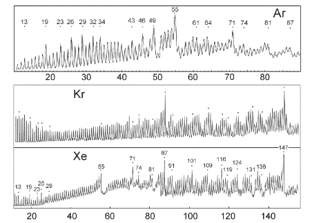
Figure 1: Experimentally measured abundance mass spectrum for the Ar, Kr and Xe clusters Echt81 ; Haberland94 ; Harris84 .

The peaks in the spectra indicate the enhanced stability of certain clusters. These clusters are called the magic clusters and their mass numbers $N$ are the magic numbers. The enhanced stability of the magic clusters can have different origin for various types of clusters. For LJ clusters, the origin of magic numbers is connected with the formation and filling the icosahedral shells of atoms. The completed icosahedral shells of atoms correspond to the following sequence of magic numbers:

$$N=\frac{10}{3}z^{3}+5z^{2}+\frac{11}{3}z+1$$ (2)

as it is clear from a simple geometry analysis. Here, the integer $z=1,2,3,4...$ is the order of the icosahedral shell. The first four icosahedral magic numbers, N, as they follow from (2) are equal to 13, 55, 147, 309. In figure 1, one can see, however, many more peaks corresponding to the formation of magic clusters having the partially completed icosahedral shells. In this paper, we elucidate the origin of all the peaks in the recorded mass spectra of the noble gas ACs in the size range up to $N\leq 150$ by modeling the mechanisms of cluster fusion and by finding in this way the most stable cluster isomers, i.e. the global energy minimum cluster structures.

To solve this problem, for each $N$, we need to find solutions of the Newton equations leading to the stable cluster configurations and then to choose the one, which is energetically the most favourable. The choice of the initial conditions for the simulation and the algorithm for the solution of this problem are described below.

Each stable cluster configuration corresponds to a minimum on the cluster potential energy surface, i.e. to the point in which all the atoms in the system are located in their equilibrium positions. A minimum can be found by allowing atoms to move, starting from a certain initial cluster configuration, and by absorbing all their kinetic energy in the most efficient way. If the starting cluster configuration for $N+1$ atoms has been chosen on the basis of the global minimum structure for $N$ atoms, then it is natural to assume, and we prove this in the present work, that very often the global minimum structure for $N+1$ atoms can be easily found. The success of this procedure reflects the fact that in nature clusters in their global minima often emerge, namely, in the cluster fusion process, which we simulate in such calculation.

We have employed the following algorithm for the kinetic energy absorption. At each step of the calculation we consider the motion of one atom only, which undergoes the action of the maximum force. At the point, in which the kinetic energy of the selected atom is maximum, we set the absolute value of its velocity to zero. This point corresponds to the minimum of the potential well at which the selected atom moves. When the selected atom is brought to the equilibrium position, the next atom is selected to move and the procedure of the kinetic energy absorption repeats. The calculation stops when all the atoms are in equilibrium.

We have considered a number of scenarios of the cluster fusion on the basis of the developed algorithm for finding the stable cluster configurations.

In the simplest scenario clusters of $N+1$ atoms are generated from the $N$-atomic clusters by adding one atom to the system. In this case the initial conditions for the simulation of $(N+1)$-atomic clusters are obtained on the basis of the chosen $N$-atomic cluster configuration by calculating the coordinates of an extra atom fussed to the system on a certain rule. We have probed the following paths: the new atom can be fussed either

(A1) to the center of mass of the cluster, or

(A2) randomly outside the cluster, but near its surface, or

(A3) to the centres of mass of all faces of the cluster, or

(A4) to the points that are close to the centres of all faces of the cluster, located from both sides of the face on the perpendicular to it, or

(A5) to the centres of mass of the faces laying on the cluster surface.

Here, the cluster surface is considered as a polyhedron, so that the vertices of the polyhedron are the atoms and two vertices are connected with an edge, if the distance between them is less than the value $d=1.2d_{0}$, where $d_{0}=2^{1/6}\sigma$ is the bonding length of a free pair of atoms. The cluster surface is considered as a polyhedron that covers all the atoms in the system and has the minimum volume. The whole cluster volume is divided on a sum of attached triangle, square and pentagonal pyramids. In the A3 method, all the faces in the cluster are counted as a sum of the faces laying on the cluster surface and the faces of the pyramids filling the cluster volume.

The choice of the method how to fuse atoms to the system depends on the problem to be solved. The A1 method is appropriate in situations when the new atoms are fused into the cluster volume. The A2 simulates the process when atoms are fused to the cluster surface. By both A1 and A2 methods, large clusters consisting of many particles can be generated rather quickly. The A2 method is especially fast, because fusion of one atom to the boundary of the cluster usually does not lead to the recalculation of its central part. The A3 and A4 methods can be used for searching the most stable, i.e. energetically favourable, cluster configurations or for finding cluster isomers with some other specific properties. The A4 method leads to finding more cluster isomers than the A3 one, but it takes more CPU time. The A5 method is especially convenient for modeling the cluster fusion process which we focus on in this paper. Using this method one can generate the cluster growth paths for the most stable cluster isomers.

In the cluster fusion process, new atoms should be added to the system starting from the initially chosen cluster configuration step by step until the desired cluster size is reached. Each new step in the cluster fusion process should be made with the use of the methods A1-A5. By methods A3-A5, one generates many different cluster isomers at each new step of the fusion process, those number grows rapidly as N increases. It is not feasible and often it is not necessary to fuse new atoms to the all found isomers. Instead, one can fuse atoms only to the selected clusters, which are of interest. Below, we outline a number of selection criteria, which can be used for the cluster selection in the fusion process depending on the problem to be solved. At each new step of the fusion process:

(SE1) one of the clusters with the minimum number of atoms is selected, or

(SE2) the cluster with the minimum energy among the already found stable clusters of the maximum size is selected, or

(SE3) a few low energy cluster isomers among the already found stable clusters of the maximum size are selected, or

(SE4) the cluster with the maximum energy among the already found stable clusters of the maximum size is selected, or

(SE5) the cluster possessing a significant structural change among the already found stable clusters is selected.

The SE1 criterion is relevant in the situation, when the full search of cluster isomers is needed. It is applicable to the systems with relatively small number of particles. Note that each cluster can be selected only once. The SE2 criterion is the most relevant for modelling the cluster fusion process and the purposes of the present work. It turns out to be very efficient and often leads to finding the most stable cluster configurations for a given number of particles. However, this is not always the case, particularly for large clusters. In these situations, the better results on the cluster global optimization can be achieved with the use of SE3 method. However, this method takes more CPU time. The SE4 and SE5 criteria turn out to be useful for the redirection of the cluster fusion process towards the lower energy cluster isomer branches.

Calculations performed with the use of the methods described above show that often clusters of higher symmetry group possess relatively low energy. Thus, the symmetric cluster configurations are often of particular interest. The process of searching for the symmetric cluster configurations can be speed up significantly, by the impose of the symmetry constraints in the cluster fusion process. This means that for obtaining a symmetric $N$ atomic cluster isomer from the initially chosen symmetric $(N-M)$-atomic configuration one should fuse $M$ atoms to the surface of this isomer symmetrically.

This goal can be achieved by various methods.

(SY1) The planes of symmetry of the parent cluster are to be found. Their intersections determine the axes of symmetry. The atoms of the parent cluster do not move and held their position, then an atom is added outside the cluster surface. The initial coordinates of it are not important, because its stable position in the vicinity of the frozen cluster surface is calculated. Then, this atom is reflected many times with respect to the found symmetry planes, and the atoms are added on the places of its images. The obtained configuration is symmetric also. After that, all the atoms in the system are allowed to move while their kinetic energy is absorbed. If the obtained stable cluster configuration is symmetric, it can be used as the initial cluster for further computations of this type. Using this procedure several times the chains of clusters of certain symmetry can be found.

(SY2) This method is similar to the one described above, but now the atoms are added to the centres of the faces on the cluster surface. If the cluster has two (or more) different types of faces, then, at first, the atoms are added to the centres of the faces of the first type and their positions are optimized with frozen cluster core. Then, the whole system is optimized and checked for symmetry. If it is symmetric, the process continues, atoms are added to the faces of the second type and the same actions are performed. This method makes possible to find more stable configurations than the first one.

(SY3) The atoms are added to the axes of symmetry outside the cluster surface. Then, the atoms of the parent cluster are assumed to be frozen and the optimized coordinates of the added atoms are calculated. After that the optimization of the whole system is performed. If the obtained cluster configuration is symmetric, it can be used as the initial cluster for further computations.

Note that the SY1-SY3 methods do not model any concrete physical scenario for the cluster fusion process. They rather represent efficient mathematical algorithms for the generation symmetrical cluster configurations, which often turn out to be very useful for the cluster structure analysis.

Note also that in addition to the cluster fusion techniques described above any stable cluster configuration can be manually modified by adding or removing a number of atoms. These modifications can also be performed using advantages of the cluster symmetry if it does exist. The manual modification of the cluster configuration is useful when the cluster geometry is already established or nearly established and only small modifications of the system are required. For example, by this method one can perform the surface rearrangement of atoms leading to the growth the number of bonds in the cluster and thus to the enhancement of its stability. This goal can be achieved by the replacement of a few loosely bound atoms on the cluster surface to the positions, in which they have larger number of bonds. As it is demonstrated in the next section, such rearrangements result in finding the cluster isomers, which alternatively can be obtained when performing the fusion simulation with the use of the SE3 criterion. The manual modifications technique requires usually much less CPU time. Cluster configurations found in this way can be used as starting configurations for the subsequent cluster fusion process.

III Results and discussions

Using our algorithms, we have examined various paths of the cluster fusion process, and determined the most stable cluster isomers for the cluster sizes of up to 150 atoms.

We have generated the chains of clusters based on the icosahedral, octahedral, tetrahedral and decahedral symmetries with the use of the A3-A5 and SE2-SE5 methods. We show that clusters possessing icosahedral and decahedral type of lattice are energetically more favourable. For the calculated cluster chains, we analyze the average interatomic distances in clusters, average number of bonds and binding energies. Using these results we explain the sequence of magic numbers, experimentally measured for the noble gas clusters, and elucidate the level of applicability of the liquid drop model for the description of the LJ cluster systems. Using the A1-A2 methods we calculate chains of energetically unfavourable cluster isomers as an example of the spontaneous cluster growth of such systems. Also, we consider the formation of symmetrical clusters using methods SY1-SY3 and their correspondence to the global energy minimum cluster structures.

III.1 Fusion of global energy minimum clusters

III.1.1 LJ cluster geometries

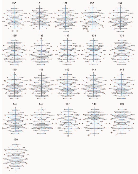
Figure 2: Growth of Lennard-Jones global energy minimum cluster structures based on the icosahedral type of packing. $LJ_{4}-LJ_{66}$ (part a), $LJ_{67}-LJ_{99}$ (part b), $LJ_{100}-LJ_{129}$ (part c) and $LJ_{130}-LJ_{150}$ (part d). The new atoms added to the cluster are marked by grey circles, while grey rings show the atoms removed.

The growth of the most stable, i.e. possessing the lowest energy, LJ clusters based on the icosahedral symmetry, the so-called global energy minimum cluster structures, is illustrated in figure 2, parts a-d. We analyse the cluster geometries within the size range $4\leq N\leq 150$ and determine the transition path from smaller clusters to larger ones. The cluster geometries have been determined using the methods described in section II. Namely, we have used A3-A5 methods combined with SE2-SE5 cluster selection criteria.

For each cluster, we show the cluster axis, i.e. a group of atoms located on a line, that goes through the cluster centre of mass. The cluster axis can be linear (see the clusters with higher symmetry, for example, $LJ_{13}$, $LJ_{55}$, $LJ_{71}$, $LJ_{147}$) or slightly distorted (see, for example, non-completed cluster configurations $LJ_{25}$, $LJ_{27}$, $LJ_{76}$, $LJ_{116}$). Other atoms in the cluster are located around the cluster axis and form the completed or open polygonal rings (see figure 2). The bonds between the atoms laying in the axis and in the rings are shown by thick and thin lines respectively. In some particular cases, we present additional connections in order to stress specific structural properties of some clusters (see, for example, $LJ_{11}$, $LJ_{31}$, $LJ_{51}$, $LJ_{82}$).

Figure 2 demonstrates how the cluster of a certain size can be obtained from the smaller one. For each cluster, we draw the added atoms by grey circles. For some clusters, it is necessary additionally to replace one atom, or even a few atoms from one position to another in order to reach the global energy minimum. In these cases, we mark the positions, from which the atoms are removed, by grey rings (see, for example, $LJ_{96}$, $LJ_{102}$, $LJ_{126}$).

Figure 2 demonstrates that the majority of energetically favourable cluster structures can be obtained with the use of the A5 method combined with the SE2 cluster selection criterion, according to which the global energy minimum cluster geometry is obtained from the preceding cluster configuration by fusion a single atom to the cluster surface. Such situation takes place for $N=$ 4-17, 19-26, 28-29, 32-34, 36-37, 39-50, 52-64, 67, 70-72, 74-75, 77, 79-81, 83, 89-92, 94-95, 97, 99-101, 103-104, 106-110, 112, 114, 116-120, 122, 124-125, 127, 129, 131-132, 134, 136-150, i.e. in about $75\%$ cases.

The global energy minimum cluster structures presented in figure 2 coincide with those found by other cluster global optimization techniques (see LesHouches ; Wales ; Leary and references therein). Note that the different choice of the constants $\varepsilon$ and $\sigma$ in various calculation schemes does not change the cluster geometry and influences only the scale of the system’s size and its total energy. However, the existing global optimization techniques do not allow to perform the cluster growth analysis, which we carry out in our work for the first time. Some preliminary results of our work have been published in GrowProcPRL ; NanoMeeting .

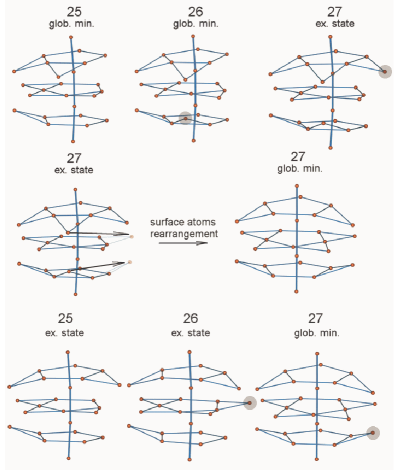
Figure 3: Fusion of a single atom to the global energy minimum cluster structure of 26 atoms does not lead to the global energy minimum of the $LJ_{27}$ cluster (first row). Rearrangement of surface atoms in the $LJ_{27}$ cluster leading to the formation of the global energy minimum cluster structure is needed (second row). The result of such rearrangement can be obtained if one starts the growth from the excited state cluster isomer of the $LJ_{25}$ cluster (third row).

It is interesting that all the calculated cluster geometries have the structure, in which a number of completed and open polygons round the cluster axis. The maximum number of atoms in polygons depends on the cluster size. Within the size range of $N\leq 150$, as it is seen from figure 2, the pentagonal, decagonal and pentadecagonal polygons are possible. The fact that this type of rings within the cluster structure dominates is closely connected with the prevalence of the icosahedral type of packing of atoms in the LJ clusters.

Note that only the clusters possessing relatively high symmetry have all the polygons rounding the axis completed. For the most of the clusters, the polygons laying close to the cluster surface are open (see e.g. $LJ_{61}$, $LJ_{89}$, $LJ_{124}$). For such clusters, the atoms added to the system occupy the positions in the open polygons located near the cluster surface.

III.1.2 Surface atoms rearrangements

Our simulations demonstrate that the fusion of a single atom to the global energy minimum cluster structure of $N$ atoms, in some cases does not immediately lead to a global energy minimum of $(N+1)$-atomic cluster. This happens for $N=$ 18, 27, 30, 35, 38, 51, 65, 66, 68, 69, 73, 76, 78, 84, 86, 87, 88, 93, 96, 98, 102, 105, 111, 113, 115, 121, 123, 126, 128, 130, 133, 135. The global energy minimum cluster structure for these cluster sizes can not be found directly with the use of A5 method combined with the SE2 criterion from the global energy minimum cluster configuration of the smaller size. In these cases the SE2 criterion leads to finding the higher energy cluster isomers, which we also call the excited state cluster isomers. In order to determine the global energy minimum cluster configurations for the above mentioned $N$, it is necessary to rearrange additionally one or a few atoms in the excited state cluster isomer (see example shown in figure 3). In figure 2, we illustrate this procedure by marking the positions of the rearranged atoms by grey circles. The initial positions of the atoms are marked by grey rings. This figure shows that the rearrangement takes place always in the vicinity of the cluster surface. This fact has a simple physical explanation. The surface atoms are bound weaker than those inside the cluster volume, and thus they are movable easier and allow the favourable surface atomic rearrangement. This consideration demonstrates that the surface rearrangement of atoms is an essential component of the cluster growth process.

We illustrate the surface rearrangement of atoms in figure 3. The first row in figure 3 shows that the fusion of a single atom to the global energy minimum cluster structure of 26 atoms does not lead to the global energy minimum of the $LJ_{27}$ cluster. Thus, the rearrangement of surface atoms in the $LJ_{27}$ cluster leading to the formation of the global energy minimum cluster structure is needed. The necessary rearrangement of atoms is shown in the second row of figure 3. The result of such rearrangement can be obtained if one starts the cluster growth from the excited state cluster isomer of the $LJ_{25}$ cluster, as it is illustrated in the third row of figure 3.

In this particular example, only the two smaller cluster sizes are involved in the fusion process of the $LJ_{27}$ cluster. However, the cluster fusion via excited states is not always that simple and evident. In some cases, it involves more than 10 intermediate steps. Such situation takes place, for example, for the $LJ_{69}$ cluster, which can be obtained from the excited state isomer of the $LJ_{55}$ cluster.

III.1.3 Average number of bonds in LJ clusters

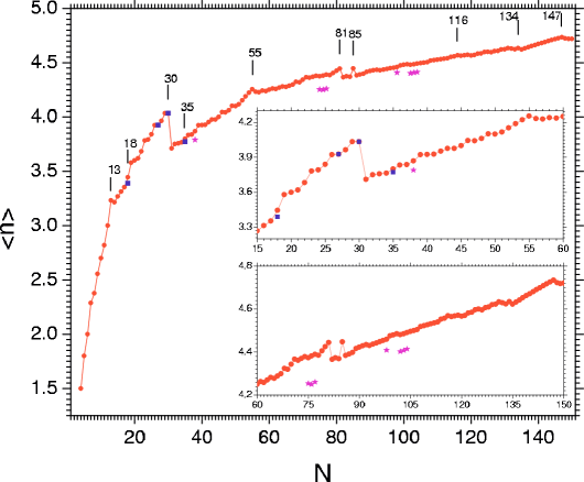
Figure 4: Average number of bonds in the icosahedral LJ global energy minimum cluster structures as a function of cluster size (circles). Squares show that for the close energy excited state cluster isomers and stars for the non-icosahedral global energy minimum cluster structures. In the insets we show in greater scale the average number of bonds in the regions $15\leq N\leq 60$ and $60\leq N\leq 150$.

The rearrangement of the surface atoms can be performed algorithmically by freezing almost all the atoms and allowing only a few atoms on the cluster surface to move. However, the number of possible cluster configurations increases rapidly with the growth cluster size, and it becomes not feasible to optimize and investigate all of them. Thus, one has to use a simple criterion for the selection of some clusters, for which the surface rearrangement of atoms is of interest. For such an analysis, we have introduced the criterion based on counting the number of bonds in the cluster. We consider the two atoms as bound if the distance between them is smaller than the given cut-off distance value $d$. Defining bonding between the atoms in such a way, we then calculate the total number of bonds in the cluster. This characteristic can be used in searching for the required cluster rearrangement, because the cluster with the maximum number of bonds, possesses the highest binding energy.

In figure 4, we present the dependence of average number of bonds in the cluster as a function of the cluster size. For this calculation we have used the cut-off value $d=1.2d_{0}$, where $d_{0}=2^{1/6}\sigma$ is the LJ potential bonding length. In figure 4, circles and squares show the average number of bonds for the global energy minimum structures presented in figure 2 and for the excited state cluster isomers with the energy close to the global minimum correspondingly. This figure demonstrates that circles always show the upper limit for the average number of bonds in the cluster.

For some clusters, like $LJ_{27}$ or $LJ_{30}$, the number of bonds in the global energy minimum cluster structure and the closest excited state cluster isomer appears to be very close. Such situations occur, when the energies of the two clusters turn out to be very close. In such cases, bonding between atoms at distances larger than the chosen cut-off value becomes important and needs to be counted in order to see that the number of bonds in the global energy minimum cluster structure is maximal. For example, the total number of bonds for the two different cluster isomers of $LJ_{30}$ calculated with the cut-off value $d$ is equal to $121$. Doubling the value of $d$ results in the total number of bonds $343$ and $339$ for the global energy minimum and the excited state cluster isomer respectively.

Such an analysis turns out to be very useful for the algorithmic search of the surface rearrangement of atoms leading to the growth of the number of bonds in the cluster and its global optimization. In simple cases, the favourable rearrangement is often obvious and it can be performed manually, by the replacement of a group of atoms from one position to another. This is often the case for larger clusters, see, for example, the rearrangement in the $LJ_{38}$ or $LJ_{69}$ clusters.

Note that the average number of bonds in the clusters with icosahedral symmetry converges to the bulk limit relatively slowly. As it is clear from a simple geometrical analysis, for an infinitively large icosahedron the average number of bonds should be equal to $6$, while for $LJ_{55}$, $LJ_{147}$ and $LJ_{309}$ it is 4.25, 4.73 and 5.00 respectively.

III.1.4 LJ cluster lattices

The methods and criteria described above appear to be insufficient for the complete description of the LJ cluster fusion process. At certain cluster sizes, a radical rearrangement of the cluster structure is necessary. Below, we call such rearrangements as the core or lattice rearrangements. Indeed, clusters in the fusion chain form the lattice of a certain type. Different lattices are based on different principles of the cluster packing and symmetry. For LJ clusters, we analyzed four different lattices: icosahedral, decahedral, octahedral and tetrahedral. The cluster configurations found in our simulations have been distinguished between the four groups according to their core symmetry. The cluster core is formed by a certain number of completed shells of atoms. Clusters consisting of the completed shells only are called the principal magic clusters. The mass numbers for the principal magic clusters (principal magic numbers) with the icosahedral, decahedral, octahedral and tetrahedral type of packing can be easily determined from simple geometric consideration and read as:

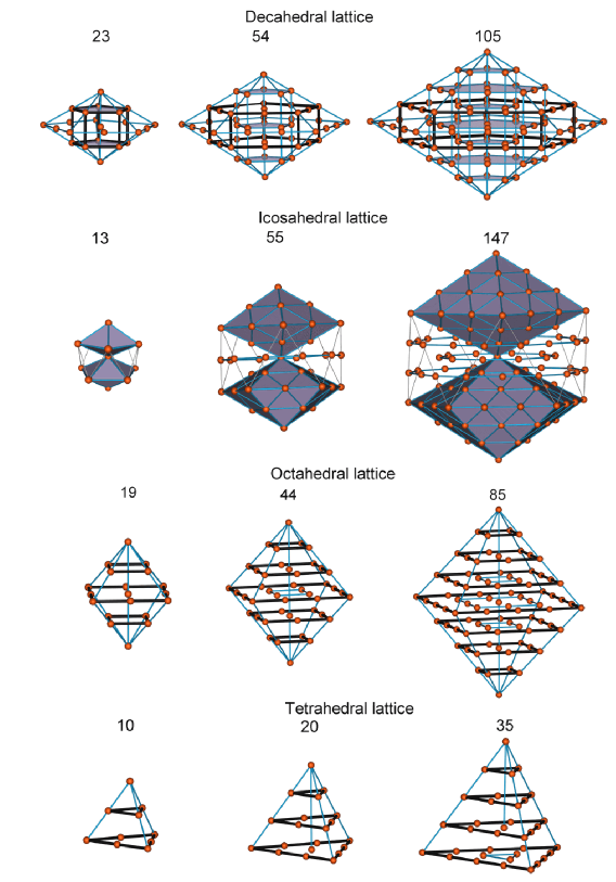
Figure 5: Geometries of magic clusters with decahedral lattice (first row), icosahedral lattice (second row), octahedral lattice (third row), tetrahedral lattice (fourth row).

$$N_{i} = \frac{10}{3}z^{3}+5z^{2}+\frac{11}{3}z+1$$ (3)

$$N_{d} = \frac{5}{6}z^{3}+\frac{5}{2}z^{2}+\frac{8}{3}z+1$$

$$N_{o} = \frac{2}{3}z^{3}+2z^{2}+\frac{7}{3}z+1$$

$$N_{t} = \frac{1}{6}z^{3}+1z^{2}+\frac{11}{6}z+1$$

where $N_{i}$, $N_{d}$, $N_{o}$ and $N_{t}$ are the principal magic numbers for the icosahedral, decahedral, octahedral and tetrahedral cluster packing, $z$ is the number of shells in the cluster or its order.

In figure 5, we show the geometrical structure of a few principal magic clusters of each type. All the clusters are formed by polygons rounding the cluster axis. Their number and type varies for different clusters.

The decahedral principal magic clusters are formed by pentagonal rings, that are located one above another along the cluster axis (see row 1 in figure 5). The number of rings and their size depends on the number of shells, $z$. Note that in decahedral clusters, the lines connecting corresponding vertices of pentagonal rings of the same size are parallel to the cluster axis.

The icosahedral principal magic clusters differ from the decahedral ones (see row 2 in figure 5). Depending on the order of cluster, the icosahedral cluster can additionally to pentagonal rings contain decagonal, pentadecagonal and etc ones. These additional rings glue together two equal decahedrons of the same order having the common axis, along which the decahedrons are turned one with respect to another on the angle $36^{o}$. As a result, some of neighbouring rings in the icosahedral clusters are also turned one with respect to another (see figure 5).

In row 3 and 4 of figure 5, we show the geometries of the principal octahedral and tetrahedral magic clusters respectively. In clusters of this type, squares and triangles correspondingly round the cluster axis.

III.1.5 LJ cluster lattice rearrangements

Let us now consider the role played by the lattice rearrangement in the formation of the global energy minimum cluster structures. Figure 2 demonstrates that the global energy minimum for $LJ_{31}$, $LJ_{82}$ and $LJ_{85}$ can not be found by the surface rearrangement of atoms.

Figure 2 clearly demonstrates that the $LJ_{31}$ cluster has obvious elements of the decahedral packing. In order to stress this fact, we connect the corresponding vertices of the pentagons by thin lines. In the clusters of the smaller size, the neighbouring pentagonal rings (completed or uncompleted) are turned one with respect to another. This feature is characteristic for the icosahedra type of cluster packing. The $LJ_{31}$ cluster structure arises in the cluster growing process via a long chain of excited state cluster isomers with $N\geq 13$. This chain is shown in figure 6. This figure demonstrates that the essential rearrangement occurs already in the $LJ_{18}$ cluster leading to the formation of the two co-ordinated pentagonal rings located one above another. After that point, the formation of the $LJ_{31}$ cluster takes place in a regular way and can be generated atom by atom.

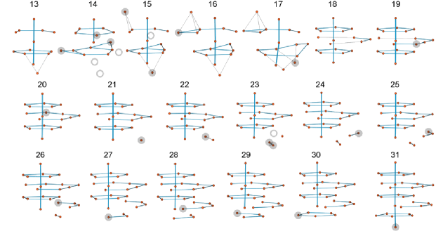
Figure 6: Formation of the $LJ_{31}$ global energy minimum structure takes place via a chain of excited state cluster isomers with $N\geq 13$. New atoms added to the system are marked by grey circles, while grey rings demonstrate the atom removal.

Figure 7: Formation of the $LJ_{82}$ global energy minimum structure involves a chain of excited state cluster isomers with $N\geq 55$. Atoms added to the system are marked by grey circles, while grey rings demonstrate the atom removal.

The next prominent rearrangement of the cluster core takes place for the $LJ_{82}$ cluster. The formation of this cluster involves a long chain of excited state cluster isomers with $N\geq 55$. In figure 7, we present this chain of clusters. The core structure for the $LJ_{82}$ cluster emerges in the $LJ_{59}$ cluster, in which the three atoms from one pentagonal ring are located just above the three atoms from another pentagonal ring (see figure 7). The further formation of the $LJ_{82}$ cluster happens in a regular manner atom by atom.

The next cluster that can not be found from the previous one by the surface rearrangement of atoms is the $LJ_{85}$ cluster. However, this cluster configuration can be easily generated starting from $LJ_{81}$ (see figure 2, part b) and using a simple rearrangement of atoms located at the cluster surface.

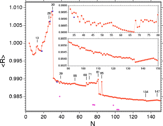
Figure 8: Average bonding length $\left<R\right>$ in the icosahedral LJ global energy minimum cluster structures as a function of cluster size (circles). Squares show $\left<R\right>$ for some excited state cluster isomers with the energy close to the global energy minimum and stars that for the non-icosahedral global energy minimum cluster structures.

To illustrate that the lattice transformations affect significantly various cluster characteristics, in figures 4 and 8, we present dependences of the average number of bonds $\left<n\right>$ and the average bonding length $\left<R\right>$ on cluster size. These figures demonstrate that for the cluster sizes $N=31$, $82$, $85$ the dependences have the step-like irregularities. These irregularities are caused by the cluster lattice rearrangements.

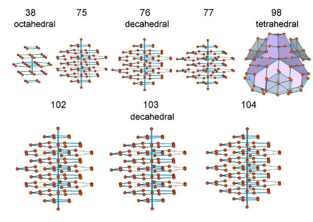
Figure 9: Geometries of non-icosahedral global energy minimum LJ clusters.

In figure 2, we present the geometries of the global energy minimum cluster structures with the icosahedral type of atomic packing. This type of packing is the most favourable for the LJ clusters. However, other type of packing is also possible and in a few cases it becomes even more favourable than the icosahedral one. Within the cluster size range considered, there are only 8 clusters for which packing other than icosahedral results in the cluster energy lower than obtained for the icosahedral clusters. These cluster structures having the octahedral, decahedral and tetrahedral type of atomic packing are presented in figure 9. They can not be obtained from their icosahedral neighbours directly. In order to find these cluster structures, one needs either to consider a chain of excited state cluster isomers analogous to the described above for the formation of the $LJ_{31}$ and $LJ_{82}$ clusters or to treat separately the growth of the octahedral decahedral and tetrahedral cluster families. Each of the cluster families should have its own magic numbers. Only a few of all these cluster configurations can compete in energy with the clusters based on the icosahedral packing as we demonstrate it in the next section. Within the size range considered such situation arises only for $N=$38, 75-77, 98, 102-104.

Note that in figures 4 and 8, we also show the average number of bonds $\left<n\right>$ and the average bonding length $\left<R\right>$ for non-icosahedral global energy minimum cluster isomers and compare these characteristics with $\left<n\right>$ and $\left<R\right>$ for clusters with icosahedral symmetry of the same size.

III.2 Cluster binding energies

The binding energy per atom for LJ clusters is defined as follows:

$$E_{b}/N=-E_{N}/N$$ (4)

where $E_{N}$ is the total binding energy of $N$-atomic cluster. In tables 1 and 2, we compile total energies and point symmetry groups for the global energy minimum cluster structures within the size range considered.

Figure 10 shows the dependence of the binding energy per atom for LJ clusters as a function of cluster size. We have generated the chains of clusters based on the icosahedral, decahedral, octahedral and tetrahedral types of lattices with the use of the A3-A5 methods combined with SE2-SE5 cluster selection criteria.

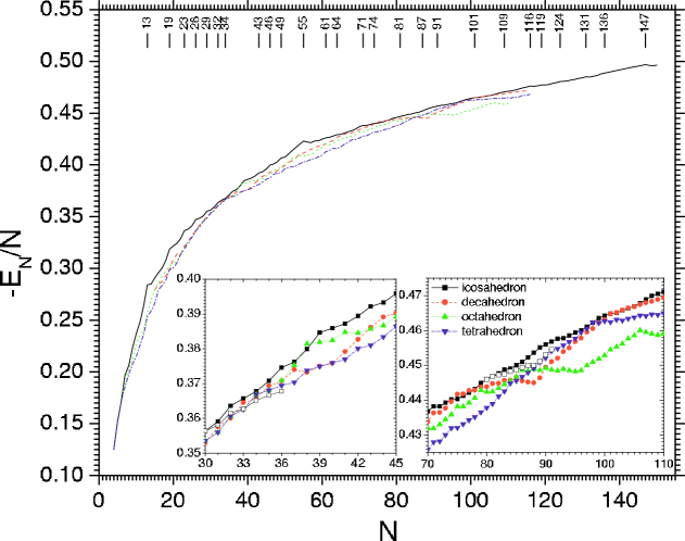
Figure 10: Binding energy per atom for LJ clusters as a function of cluster size calculated for the cluster chains based on the icosahedral (solid line), octahedral (doted line), tetrahedral (dash dotted line) and decahedral (dashed line) types of packing. In the insets we show the behaviour of the curves in the regions $30\leq N\leq 45$ and $70\leq N\leq 110$ in which energies of the clusters with different type of packing become especially close. We also present the energies for the chains of clusters growing up from $LJ_{30}$ and $LJ_{81}$ without rearrangement of their lattice (opened squares).

Figure 10 shows that the most stable clusters are mostly based on the icosahedral type of packing with exceptions for $N=38$, $75\leq N\leq 77$, $98$ and $102\leq N\leq 104$. In these cases the octahedral, decahedral, tetrahedral and again decahedral cluster symmetries respectively become more favourable. To illustrate this, in the insets to figure 10, we show the behaviour of the curves in the regions $30\leq N\leq 45$ and $70\leq N\leq 110$ in greater detail. In these regions, energies of the clusters with different type of packing become especially close.

In previous section, we have demonstrated that the structural cluster properties experience dramatic change at $N=31$, $82$, $85$. In the contrary to the structural characteristics, the dependence of binding energy per atom on $N$ behaves smoothly in the vicinity of these points. In order to stress the role of the cluster lattice rearrangement in the formation of the global energy minimum cluster structures, in the inset to figure 10, we plot by open squares the energies for the chains of clusters growing up from $LJ_{30}$ and $LJ_{81}$ without rearrangement of their lattice. Clusters in these chains become more and more energetically unfavourable with the growth cluster size as compared to the global energy minimum structures.

On the top of figure 10 we present the sequence of magic numbers experimentally measured for noble gases Echt81 ; Haberland94 . It is seen that the magic numbers correspond to the peculiarities in the curve for the binding energy per atom as a function of cluster size calculated for the cluster chain based on the icosahedral type of packing. The peculiarities indicate the enhanced stability of the corresponding clusters. Note that in experiment the magic numbers are seen much better in the regions of $N$, in which the icosahedrally packed clusters are energetically the most favourable. The most prominent peculiarities arise for the completed icosahedral shells with 13, 55 and 147 atoms. The peculiarities in the dependence of binding energy per atom on $N$ diminish with the growth of the cluster size due to approaching to the bulk limit, in which the binding energy per atom is constant.

III.3 Liquid drop model

The main trend of the energy curves plotted in figure 10 can be understood on the basis of the liquid drop model, according to which the cluster energy is the sum of the volume and the surface energy contributions:

$$E_{N}=-\lambda_{V}N+\lambda_{S}N^{2/3}-\lambda_{R}N^{1/3}$$ (5)

Here the first and the second terms describe the volume, and the surface cluster energy correspondingly. The third term is the cluster energy arising due to the curvature of the cluster surface. Choosing constants in (5) as $\lambda_{V}=0.71554$, $\lambda_{S}=1.28107$ and $\lambda_{R}=0.5823$, one can fit the global energy minimum curve plotted in figure 10 with the accuracy less than $1\%$. The deviations of the energy curves calculated for various chains of cluster isomers from the liquid drop model (5) are plotted in figure 11. We have fited the energies of the icosahedral clusters in the cluster size range $4\leq N\leq 150$ using the nonlinear least squares fitting method.

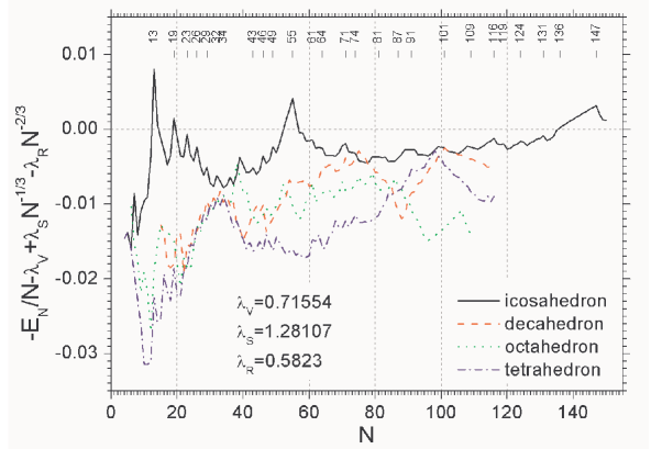
Figure 11: Energy curves deviations from the liquid drop model (5) calculated for the cluster chains based on the icosahedral (solid line), octahedral (doted line), tetrahedral (dash dotted line) and decahedral (dashed line) type of packing.

The peaks on these dependences indicate the increased stability of the corresponding magic clusters. The ratio between the volume and surface energies in (5) can be characterised by the dimensionless parameter $\delta=\lambda_{V}/\lambda_{S}$, being equal in our case to $\delta=0.559$. Note, that this value slightly differs from the previously reported in GrowProcPRL , $\delta_{PRL}=0.555$, which was obtained by fitting the cluster global energy minima within the same cluster size range.

This result can be compared with those published in Doye . In this paper the energy of the first four completed icosahedral shells was fitted using equation (5). This fitting gives the value $\delta=0.576$ differing from our result due to the difference in the fitting method. In Doye the energies of the 4 selected clusters have been used, while we fit the energies of all the clusters within the size range $4\leq N\leq 150$

Note that a similar model is used in nuclear physics for the description of the nuclei binding energy. For the nuclear matter, the constant $\delta$ is equal to $\delta=0.903$ BM .

III.4 Cluster magic numbers

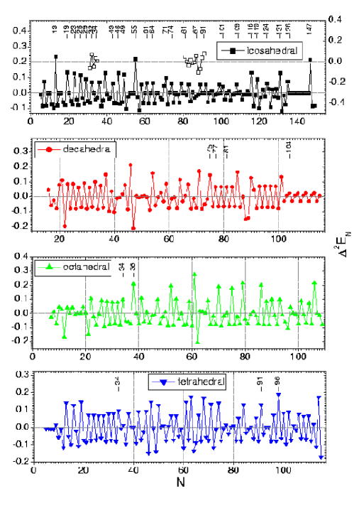
Figure 12: Second derivatives $\Delta^{2}E_{N}$ for the icosahedral (squares), decahedral (circles), octahedral (upper triangles) and tetrahedral (lower triangles) cluster isomer chains. Open squares show $\Delta^{2}E_{N}$ for the chains of energetically unfavourable clusters growing from $LJ_{30}$ and $LJ_{81}$ without rearrangement of their lattice.

The dependence of the binding energies per atom for the most stable cluster configurations on $N$ allows one to generate the sequence of the cluster magic numbers. In figure 12, we plot the second derivatives $\Delta^{2}E_{N}$ for the cluster chains with icosahedral, decahedral, octahedral and tetrahedral type of packing.

We compare the obtained dependences with the experimentally measured abundance mass spectra for the noble gas clusters Echt81 ; Haberland94 (see figure 1) and establish the striking correspondence of the peaks in the experimentally measured mass spectra with those in the $\Delta^{2}E_{N}$ dependence calculated for the icosahedral type of clusters. The sequence of the magic numbers for the Ar, Xe and Kr clusters reads: 13, 19, 23, 26, 29, 32, 34, 43, 46, 49, 55, 61, 64, 71, 74, 81, 87, 91, 101, 109, 116, 119, 124, 131, 136, 147 Echt81 ; Haberland94 . The most prominent peaks in this sequence 13, 55 and 147 correspond to the closed icosahedral shells, while other numbers correspond to the filling of various parts of the icosahedral shell.

The connection between the second derivatives $\Delta^{2}E_{N}$ and the peaks in the abundance mass spectrum of clusters one can understand using the following simple model. Let us assume that the mass spectrum of clusters is formed in the evaporation process. This means that changing the number of clusters $n_{N}$ of the size $N$ in the cluster ensemble takes place due to the evaporation of an atom by the clusters of the size $N$ and $N+1$, i.e.

$$\Delta n_{N}\sim n_{N+1}W_{N+1\rightarrow N}-n_{N}W_{N\rightarrow N-1}$$ (6)

where the evaporation probabilities are proportional to

$$W_{N+1\rightarrow N} \sim e^{-\frac{E_{N}+E_{1}-E_{N+1}}{kT}}$$ (7)

$$W_{N\rightarrow N-1} \sim e^{-\frac{E_{N-1}+E_{1}-E_{N}}{kT}}$$

Here $T$ is the cluster temperature, $k$ is the Bolzmann constant. In our model $E_{1}=0$, so after simple transformations the equation for $\Delta n_{N}$ reads as:

$$\Delta n_{N} \sim n_{N+1}e^{-\frac{E_{N}-E_{N+1}}{kT}}(1-\frac{n_{N}}{n_{N+1}}e^{-\frac{E_{N-1}-2E_{N}+E_{N+1}}{kT}})$$

$$\sim n_{N}e^{-\frac{E_{N}-E_{N+1}}{kT}}(1-e^{-\frac{E_{N-1}-2E_{N}+E_{N+1}}{kT}})$$

Here we assumed that $n_{N+1}\sim n_{N}\sim n_{N-1}\gg 1$. Let us now estimate the relative abundances in the mass spectrum for Ar clusters for temperatures about 100 K. The exponent $e^{-\frac{E_{N}-E_{N+1}}{kT}}$ influences the absolute value of $\Delta n_{N}$. This factor becomes exponentially small at $kT\ll E_{N}-E_{N+1}$, which for the Ar clusters means $T\ll 800K$, because $\left<\Delta E_{N}^{Ar}\right>=0.071eV\sim 800K$. The small value of this factor results in the growth of the characteristic period of the evolution of $n_{N}$ with time. The factor in the brackets determines the relative cluster abundances. Indeed, its positive value for certain $N$ leads to the growth of the corresponding clusters in the system, while the negative value of the factor to the opposite behaviour. The factor in the brackets is characterised by $\Delta^{2}E_{N}=E_{N-1}-2E_{N}+E_{N+1}$, which is for the Ar clusters $\left<|\Delta^{2}E_{N}|\right>=0.008eV\sim 90K$. Thus, for temperatures $T\gtrsim 90K$ the exponent in the brackets can be expanded. In this case one derives

$$\Delta n_{N}\sim n_{N}e^{-\frac{E_{N}-E_{N+1}}{kT}}\frac{\Delta^{2}E_{N}}{kT}$$ (9)

This equation demonstrates, that positive values of $\Delta^{2}E_{N}$ leads to the enhanced abundance of the corresponding clusters.

For Xe and Kr clusters this approximation becomes applicable at somewhat larger $T$, because the depth of the LJ potential, $\varepsilon$, for this type of clusters, is larger than for Ar clusters. For Ar clusters $\varepsilon=12.3$ meV while for Kr and Xe it is $17.2$ and $24.3$ meV respectively.

Within the size range considered there are only five magic numbers, which can not be directly explained on the basis of $\Delta^{2}E_{N}$ calculated for the chain of icosahedral clusters. This situation takes place for $N=$34, 81, 87, 91 and 136. However, the origin of these magic numbers can also be understood.

The magic number $N=$34 is not seen in the chain of the energetically most favourable icosahedral clusters, because of the lattice rearrangement that occurs for $N=$31. Beginning from $LJ_{31}$ a new cluster growing chain becomes energetically more favourable, but the chain of clusters growing from $LJ_{30}$ without its lattice rearrangement turns out to be rather close to the global energy minimum chain (see figure 10). As a result, in the vicinity of the transition point both chains influence the magic number formation. Thus, for $N=$34, the positive peak in the $\Delta^{2}E_{N}$ for the chain of the global minimum clusters is absent, but it for present in the chain of clusters growing from the $LJ_{30}$ cluster without its lattice rearrangement (see open squares in figure 12). This magic number can also be seen for the octahedral and tetrahedral cluster chains, which come energetically rather close to the icosahedral chain in this region of $N$.

For the $LJ_{81}$ cluster the situation is similar. Here again a structural rearrangement of the cluster lattice takes place influencing the magic number formation. Thus, the magic numbers 81, 87, 91 arise in the chain of clusters growing from the $LJ_{81}$ cluster without its lattice rearrangement. The number 81 arises also in the chain of the decahedral clusters, which in this region of $N$ is energetically close to the global energy minimum (see figure 12). The chain of tetrahedral clusters affects the formation of the 91 magic number due to the same reason. Though this magic number is absent in the sequence of magic numbers generated for global energy minimum cluster structures, it is well pronounced in the magic number sequence for the tetrahedral clusters and the chain of clusters growing from $LJ_{81}$ without its lattice rearrangement.

Another magic number, which is masked in the magic number sequence for the icosahedral clusters is $N=$136. This number is masked because of the radical surface rearrangement of atoms needed for obtaining its configuration from the $LJ_{135}$ one. The $LJ_{135}$ cluster is the truncated 147 icosahedron. It possesses the $I_{h}$ point symmetry group. It can be obtained from the $LJ_{134}$ cluster by a rearrangement of 7 atoms located on the cluster surface. This cluster configuration can be obtained via a long chain of excited state cluster configurations which starts from the $LJ_{55}$ icosahedral cluster. In experiment, the formation of the global energy minimum $LJ_{135}$ cluster structure should occur with relatively low probability because of the reasons outlined above. Instead, it is feasible to assume that for this particular cluster size different cluster isomers with energies close to the global minimum can be readily created. This influences the 135 magic number formation resulting in its shift to $N=136$.

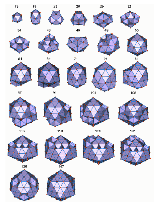
Figure 13: Geometries of the magic LJ clusters. The labels indicate the cluster size.

Note that $\Delta^{2}E_{N}$ values calculated for the chain of icosahedral clusters in the size range $136\leq N\leq 146$ are very close to zero. This fact can be explained as follows. There are 12 vacancies in the outer icosahedral shell of the $LJ_{135}$ cluster, which are located at the vertices of the $LJ_{147}$ icosahedron. These vacancies are sequentially filled within the size range $136\leq N\leq 146$. Within this size range the energy difference between the two neighbouring clusters practically does not vary and is determined by the energy of an atom placed in one of the icosahedron vertice vacancies. Such a situation takes place, because the distances between any of two vertices are much larger than the pairing bond length in the LJ potential and the interaction between the atoms placed in the icosahedron vertices is neglible. As a result, of this the total energy grows nearly linearly and $\Delta^{2}E_{N}\approx 0$

In figure 13, we plot images of the magic global energy minimum cluster structures. In this figure it is clearly seen how one icosahedral shell emerges from another. This figure demonstrates that the process of the $LJ_{55}$ icosahedron cluster formation has similarities with the formation of the $LJ_{147}$ cluster. In both cases, at the first stage a cap is formed on the top of the completed icosahedron shell, see the $LJ_{19}$ and $LJ_{71}$ magic clusters. Then, in both cases a structural rearrangement of the cluster takes place. When the rearrangement of the cluster lattice is completed ($LJ_{31}$, $LJ_{82}$), the growth of the cluster occurs by filling the atomic vacancies in the vicinity of the cluster surface up to the point when a new icosahedral shell is formed.

We have demonstrated that the magic numbers for the icosahedral clusters map well enough the experimentally observed magic numbers. In figure 9, we present the images of the non icosahedral global energy minimum cluster structures. Experimentally these clusters are not found to be the magic clusters, although, they are the global minimum clusters being magic for the chains of clusters based on the decahedral, octahedral or tetrahedral type of packing (see figures 10 and 12). This fact can be understood if one takes into account that the chains of clusters with different type of atomic packing are formed independently and the transition of clusters from one chain to another at certain $N$ occurs with the small probability. From the binding energy analysis, it is clear that the chain of icosahedral clusters prevails. Thus, in experiment, the icosahedral clusters mask the clusters belonging to the chains of non-icosahedraly packed clusters, even when the non-icosahedral cluster structures happen to become energetically more favourable.

III.5 Spontaneous cluster fusion

Using the A2 method and the SE2 cluster selection criterion we have generated a chain of energetically unfavourable cluster isomers with $N\leq 84$ as an example of the spontaneous cluster growth.

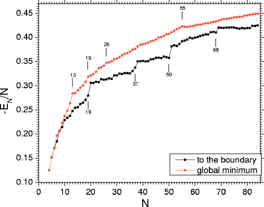
Figure 14: Binding energies per atom for a chain of spontaneously produced clusters in comparison with the binding energies per atom for the global energy minimum cluster structures.

In figure 14, we compare the binding energies per atom for the chain of the spontaneously produced clusters with the binding energies per atom calculated for the global energy minimum cluster structures. This figure shows that the binding energy per atom for the spontaneously generated cluster structures are systematically lower than those for the global energy minimum structures. However, the two dependences behave quite differently. Thus, at certain cluster sizes, the binding energy per atom for the spontaneously generated chain of clusters increases in a step-like manner. In the size range considered, this occurs for the cluster sizes $N=19-20,$ $37-38$, $50-51$, $68-69$, $81-82$. These irregularities originate from the significant structural rearrangement taking place in the spontaneously generated cluster structures. In figure 15, we illustrate such a rearrangement for the clusters with $N=19-20$ and $N=68-69$.

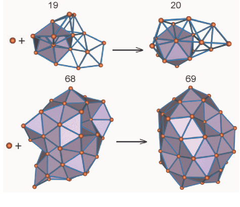
Figure 15: Structural rearrangements in spontaneously generated cluster structures with $N=19-20$ and $N=68-69$. Fusion of just one atom to the cluster boundary rearranges its structure and leads to the formation of a stable cluster core.

The structural rearrangement in the $LJ_{19}$ cluster leads to the formation of the compact 13-atomic icosahedron shell. Indeed, in the initial $LJ_{19}$ cluster isomer, only a part of the icosahedron can be identified (see figure 15). Fusion of just one atom to the cluster boundary rearranges its structure and forms the compact icosahedral shell as a cluster core. This transformation stabilizes the cluster structure and makes it energetically much more favourable.

The situation with the $LJ_{68}$ cluster is similar. Again, we consider a highly asymmetric cluster isomer (see figure 15), which deviates significantly from the global energy minimum cluster structure based on the 55-atomic icosahedron shell (see figure 2). Fusion of a single atom to the boundary of the initial cluster configuration rearranges its structure completely forming a relatively compact $LJ_{69}$ cluster isomer (see figure 15). The $LJ_{69}$ cluster configuration possesses the evident elements of the 55-atomic icosahedron shell, which are absent in the initial $LJ_{68}$ cluster isomer. The compact configuration of the found $LJ_{69}$ cluster isomer brings its binding energy per atom close to the binding energy per atom calculated for the global energy minimum cluster structure.

III.6 Symmetrical cluster fusion

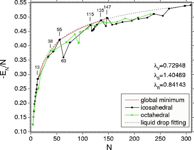
Figure 16: Binding energies per atom for sequences of symmetrical clusters with icosahedral (squares) and octahedral (triangles) types of packing and their comparison with the binding energies per atom for the global energy minimum cluster structures (solid line) and the liquid drop model (5) fitting (dotted line).

Using the SY1-SY3 methods, we now consider the formation of symmetrical clusters and perform their energy analysis. We have generated the cluster configurations with $N\leq 309$ possessing the icosahedral and octahedral symmetry.

In figure 16, we plot the binding energies per atom calculated for clusters possessing the icosahedral and octahedral symmetry and compare them with the binding energies per atom calculated for the global energy minimum cluster structures. Figure 16 demonstrates the irregular behaviour of the binding energies of the calculated symmetrical cluster configurations. Note that this irregularities are not of the physical nature, because the SY1-SY3 methods do not model any concrete physical scenario of the cluster fusion process. These methods rather represent an efficient mathematical algorithm for the generation of symmetrical cluster configurations (see section II for details).

It is interesting that some of the found symmetrical cluster configurations within the size range $N\leq 150$ appear to be the global energy minimum cluster structures. This is the case for the clusters with $N=$13, 55, 135, 147, possessing the icosahedral point symmetry group, $I_{H}$. The binding energy of the highly symmetrical cluster isomer $LJ_{115}$ possessing also the $I_{H}$ point symmetry group is only about $0.0033$ units smaller than the energy of the corresponding global energy minimum. It is interesting that the $LJ_{115}$ global energy minimum cluster structure possesses the $C_{5V}$ point symmetry group, being lower than the $I_{H}$ point symmetry group. The fact that the cluster isomer with the lower symmetry becomes energetically more favourable can be understood after counting the total number of bonds in the system (see section III.1 for details). In the $LJ_{115}$ icosahedral isomer the total number of bonds is equal to 524, while in the global energy minimum isomer it is equal to 534. Here we have used the cut-off value equal to $d=1.2\cdot 2^{1/6}\sigma$. Comparison of the two number shows that the large number of bonds can be created in a system with the lower symmetry and that the larger number of bonds means the higher stability of the system.

Among the octahedral cluster configurations found with the use of the same technique there are also a few ones with the energy being very close to the cluster global energy minimum. Thus, the truncated octahedron $LJ_{38}$ appears to be the only global energy minimum cluster structure within the size range of $N\leq 150$ possessing the octahedral symmetry (see section III.1 for more details). The $LJ_{116}$ cluster isomer has also the form of truncated octahedron. Its binding energy is smaller than the binding energy of the global energy minimum cluster structure of the same size on $0.0024$ unit.

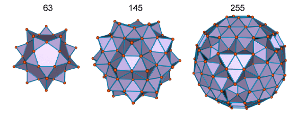
Figure 17: Clusters with icosahedral point symmetry group having low binding energy per atom.

Note that some highly symmetric clusters, like the icosahedral $LJ_{63}$, $LJ_{145}$, $LJ_{255}$ can have relatively low binding energy as compared to their neighbours (see figure 16). The geometries of these clusters are shown in figure 17. They appear to be relatively low stable, because the total number of bonds in these clusters (222, 654 and 1194 respectively) is significantly lower than it is in the corresponding global energy minimum cluster structures (269 for $LJ_{63}$, 684 for $LJ_{145}$, for $LJ_{255}$ the total number of bonds in the global energy minimum is not known).

The calculation of the symmetrical cluster configuration and their energies turns out to be very useful for the preliminary analysis of the binding energy curve in a wide range. Thus, fitting the points $N=13,55,115,135,147,267,297,309$ with use of the liquid drop model equation (5), one derives the following values of $\lambda_{V}=0.72948$, $\lambda_{S}=1.40469$, $\lambda_{R}=0.84143$, which are in a good agreement with the results following from the global energy minimum calculations, see section III.3. We note that the performed analysis of symmetrical cluster configurations is essentially easier than the complete analysis of the global energy minima and thus it can be used for the efficient calculation of cluster binding energies in a wide range of $N$ at relatively high level of accuracy.

IV Conclusion

In this paper we have discussed the classical models for the cluster growing process, but our ideas can be easily generalized on the quantum case and be applied to the cluster systems with different than LJ type of the inter-atomic interaction. It would be interesting to see to which extent the parameters of inter-atomic interaction can influence the cluster growing process and the corresponding sequence of magic numbers or whether the crystallization in the nuclear matter consisting of alpha particles and/or nucleons is possible. Studying cluster thermodynamic characteristics with the use of the developed technique is another interesting problem which is left open for future considerations.

V Acknowledgments

The authors acknowledge support of this work by the Studienstiftung des deutschen Volkes, Alexander von Humbolt Foundation, DFG, Russian Foundation of Basic Research, Russian Academy of Sciences and the Royal Society of London.

Appendix A Algorithm details

In this section we provide some details of the algorithms used in the computations NanoMeeting .

In the described algorithm, the potential energy of selected atom decreases during its motion. Therefore, the total potential energy of the cluster decreases at each step of the algorithm and it finally converges to a stable cluster configuration. In most cases, this convergence is rather fast. The time required for the obtaining of a stable configuration with the error $\Delta E$ of the potential energy is usually proportional to $-ln\Delta E$. To speed up the process of conversion the procedure for the determination of the LJ force acting on the atom was written in Assembler x86. The performance of the calculations increased approximately 1.5 times comparing to the version written entirely in C.

Note that the described algorithm of the kinetic energy absorption is much more efficient as compared to those reducing the kinetic energy of moving atoms at each step of the Runge-Kutta integration procedure. Firstly, the following method was used: during the motion on each Runge-Kutta step the speed of an atom was decreased $k$ times. Therefore, the whole energy of oscillations that occur near the equilibrium position decreases because of the decreasing of the kinetic energy. So far, when the speed becomes very small, atoms start to oscillate very close to the potential energy minimum position. This method is rather simple, but too much time is required for atom coordinates to converge to their equilibrium position. Therefore we introduced another sufficient energy absorption algorithm, that was described in section II.

To prevent the fragmentation of the cluster caused by the unfavourable initial conditions, the adaptive choice of time-step in the Runge-Kutta integration procedure has been implemented. The fragmentation of the system might happen, for example, in the case when initially a pair of atoms are placed at a small distance one from another so that they experience a very strong repulsive force. In such a situation the moving atom gains high acceleration and during the first step of the Runge-Kutta procedure might go far away from the cluster. If the force acting on this atom in its final position is smaller than a given value $F_{min}$, it will be assumed in equilibrium and it will never be attracted back to the cluster, although the final configuration won’t be stable. The adaptive choice of the integration time-step prevents the atoms to fly apart. The idea of this procedure is rather simple. Each time step $\Delta t$ in the Runge-Kutta integration procedure is repeated with the time step $\Delta t/2$. If the coordinate or velocity change on the interval $\Delta t/2$ is found too large then the integration step $\Delta t$ is reduced and the procedure repeats. If the coordinate change is too small than the larger value of the interval $\Delta t$ is set and the calculation is repeated again. The adaptive choice of the integration time step prevent the atoms to fly away, because in the unfavourable initial conditions situation the integration time-steps will become small, though the velocity will be high. Nevertheless, when the atom reaches the boundary of the cluster, it will stop: at that moment its velocity starts to decrease because of the attraction to the cluster.

Appendix B Tables

Table 1: Total energies and point symmetry groups for LJ global energy minimum isomers within the size range $4\leq N\leq 78.$

N	Point group	Energy	N	Point group	Energy	N	Point group	Energy
4	$T_{D}$	-0.500000	29	$D_{3H}$	-10.29895	54	$C_{5V}$	-22.68405
5	$D_{3H}$	-0.758654	30	$C_{2V}$	-10.69055	55	$I_{H}$	-23.27071
6	$O_{H}$	-1.059339	31	$C_{S}$	-11.13220	56	$C_{3V}$	-23.63693
7	$D_{5H}$	-1.375449	32	$C_{2V}$	-11.63629	57	$C_{S}$	-24.02855
8	$C_{S}$	-1.651791	33	$C_{S}$	-12.07023	58	$C_{3V}$	-24.53151
9	$C_{2V}$	-2.009447	34	$C_{2V}$	-12.50371	59	$C_{2V}$	-24.97817
10	$C_{3V}$	-2.368544	35	$C_{1}$	-12.97972	60	$C_{S}$	-25.48962
11	$C_{2V}$	-2.730498	36	$C_{S}$	-13.48545	61	$C_{2V}$	-26.00074
12	$C_{5V}$	-3.163967	37	$C_{1}$	-13.91947	62	$C_{S}$	-26.44616
13	$I_{H}$	-3.693900	38	$O_{H}$	-14.49404	63	$C_{1}$	-26.95748
14	$C_{3V}$	-3.987096	39	$C_{5V}$	-15.00277	64	$C_{S}$	-27.46835
15	$C_{2V}$	-4.360219	40	$C_{S}$	-15.43749	65	$C_{2}$	-27.91429
16	$C_{S}$	-4.734645	41	$C_{S}$	-15.87802	66	$C_{1}$	-28.42588
17	$C_{2}$	-5.109833	42	$C_{S}$	-16.35646	67	$C_{S}$	-28.93767
18	$C_{5V}$	-5.544246	43	$C_{S}$	-16.86372	68	$C_{1}$	-29.44955
19	$D_{5H}$	-6.054982	44	$C_{1}$	-17.30739	69	$C_{5V}$	-29.99021
20	$C_{2V}$	-6.431420	45	$C_{1}$	-17.81541	70	$C_{5V}$	-30.57435
21	$C_{2V}$	-6.807048	46	$C_{2V}$	-18.39003	71	$C_{5V}$	-31.11247
22	$C_{S}$	-7.234149	47	$C_{1}$	-18.83435	72	$C_{S}$	-31.55310
23	$D_{3H}$	-7.737039	48	$C_{S}$	-19.34996	73	$C_{S}$	-32.06578
24	$C_{S}$	-8.112401	49	$C_{3V}$	-19.92432	74	$C_{S}$	-32.57571
25	$C_{S}$	-8.531055	50	$C_{S}$	-20.37916	75	$D_{5H}$	-33.12436
26	$T_{D}$	-9.026301	51	$C_{2V}$	-20.93783	76	$C_{S}$	-33.57457
27	$C_{2V}$	-9.406132	52	$C_{3V}$	-21.51917	77	$C_{2V}$	-34.09029
28	$C_{S}$	-9.818533	53	$C_{2V}$	-22.10025	78	$C_{S}$	-34.56620

Table 2: The same as table 1 but within the size range $79\leq N\leq 150$.

N	Point group	Energy	N	Point group	Energy	N	Point group	Energy
79	$C_{2V}$	-35.15091	104	$C_{2V}$	-48.50722	129	$C_{S}$	-62.37172
80	$C_{S}$	-35.67363	105	$C_{1}$	-49.02221	130	$C_{1}$	-62.93926
81	$C_{2V}$	-36.19530	106	$C_{1}$	-49.58842	131	$C_{2V}$	-63.53680
82	$C_{1}$	-36.71254	107	$C_{S}$	-50.16726	132	$C_{1}$	-64.00352
83	$C_{2V}$	-37.24367	108	$C_{S}$	-50.75275	133	$C_{S}$	-64.58527
84	$C_{1}$	-37.72143	109	$C_{1}$	-51.28426	134	$C_{3V}$	-65.18385
85	$C_{3V}$	-38.25465	110	$C_{S}$	-51.81566	135	$I_{H}$	-65.85651
86	$C_{1}$	-38.78204	111	$C_{S}$	-52.33903	136	$C_{5V}$	-66.45444
87	$C_{S}$	-39.34151	112	$C_{S}$	-52.90622	137	$C_{2V}$	-67.05262
88	$C_{S}$	-39.91939	113	$C_{S}$	-53.48289	138	$C_{3V}$	-67.65107
89	$C_{3V}$	-40.50449	114	$C_{S}$	-54.06942	139	$C_{2V}$	-68.24949
90	$C_{S}$	-41.03616	115	$C_{5V}$	-54.64636	140	$C_{S}$	-68.84789
91	$C_{S}$	-41.56759	116	$C_{5V}$	-55.23411	141	$C_{5V}$	-69.44655
92	$C_{3V}$	-42.09876	117	$C_{1}$	-55.69023	142	$C_{S}$	-70.04488
93	$C_{1}$	-42.57314	118	$C_{S}$	-56.23080	143	$C_{2V}$	-70.64347
94	$C_{1}$	-43.10534	119	$C_{S}$	-56.78493	144	$C_{3V}$	-71.24204
95	$C_{1}$	-43.63668	120	$C_{1}$	-57.25183	145	$C_{2V}$	-71.84058
96	$C_{1}$	-44.15660	121	$C_{1}$	-57.81830	146	$C_{5V}$	-72.43938
97	$C_{1}$	-44.72345	122	$C_{1}$	-58.41161	147	$I_{H}$	-73.03843
98	$T_{D}$	-45.30545	123	$C_{S}$	-58.98351	148	$C_{S}$	-73.42275
99	$C_{2V}$	-45.88888	124	$C_{S}$	-59.57674	149	$C_{S}$	-73.89112
100	$C_{S}$	-46.41998	125	$C_{S}$	-60.10860	150	$C_{3V}$	-74.44252
101	$C_{2V}$	-46.95094	126	$C_{1}$	-60.61249
102	$C_{2V}$	-47.44697	127	$C_{2V}$	-61.20664
103	$C_{S}$	-47.98051	128	$C_{1}$	-61.77768

References

References

- (1) NATO Advanced Study Institute, Les Houches, Session LXXIII, Summer School ”Atomic Clusters and Nanoparticles” (Les Houches, France, July 2-28, 2000), Edited by C. Guet, P. Hobza, F. Spiegelman and F. David, EDP Sciences and Springer Verlag, Berlin, Heidelberg, New York, Barcelona, Hong Kong, London, Milan, Paris, Tokyo (2001).
- (2) W.D. Knight, K. Clemenger, W.A. de Heer, W.A. Saunders, M.Y. Chou and M.L. Cohen, Phys. Rev. Lett. 52, 2141 (1984)
- (3) W. Ekardt (ed.), Metal Clusters (Wiley, New York ,1999)
- (4) H.W. Kroto et al., Nature 318, 163 (1985)
- (5) J. Kirkpatrick, Jr., C.D. Gelatt, and M.P. Vecchi Science 220, 671 (1983)
- (6) L.T. Wille, Chem. Phys. Lett. 133, 405 (1987)
- (7) J. Ma, D. Hsu, and J.E. Straub J. Chem. Phys. 99, 4024 (1993)
- (8) J. Ma, and J.E. Straub J. Chem. Phys. 101, 533 (1994)
- (9) C. Tsoo, and C.L. Brooks J. Chem. Phys. 101, 6405 (1994)
- (10) P.J.M. van Laaarhoven, and E.H.L. Aarts Simulated Annealing: Theory and Applications (Reidel, Dordrecht ,1987)
- (11) M.H. Kalos, and P.A. Whitlock Monte Carlo Methods (Wiley, New York ,1986)
- (12) A.B. Finnila, M.A. Gomez, C. Sebenik, C. Stenson, and J.D. Doll Chem. Phys. Lett. 219, 343 (1994)
- (13) P. Amara, D. Hsu, and J.E. Straub J. Chem. Phys. 97, 6715 (1993)
- (14) P. Amara, D. Hsu, and J.E. Straub J. Chem. Phys. 95, 4147 (1991)
- (15) C.D. Maranas, and C.A. Floudas J. Chem. Phys. 97, 7667 (1992)
- (16) C.D. Maranas, and C.A. Floudas J. Chem. Phys. 100, 1247 (1994)
- (17) F.H. Stillinger, and T.A. Webber J. Stat. Phys. 52, 1429 (1988)
- (18) L. Piela, K.A. Olszewski and J. Pillardy J. Mol. Struct. 308, 229 (1994)
- (19) J. Pillardy, K.A. Olszewski and L. Piella J. Phys. Chem. 96, 4337 (1992)
- (20) D.J Wales and J.P.K. Doye J. Phys. Chem. A 101, 5111 (1997)
- (21) R.H Leary and J.P.K. Doye Phys. Rev. E 60, 6320 (1999)
- (22) D.E. Goldberg Genetic Algorithms in Search, Optimization, and Machine Learning (Addison-Wesley, Reading, MA, 1989)
- (23) J.A Niesse and H.R. Mayne J. Chem. Phys. 105, 4700 (1996)
- (24) S.K Gregurick, M.H. Alexander and B. Hartke J. Chem. Phys. 104, 2684 (1996)
- (25) D.M Deaven, N. Tit, J.R Morris and K.M. Ho Chem. Phys. Lett. 256, 195 (1996)
- (26) D. Romero, C. Barron, S. Gomez Comp. Phys. Comm. 123, 87 (1999)
- (27) Il.A. Solov’yov, A.V. Solov’yov, W. Greiner et al, Phys. Rev. Lett. 90, 053401 (2003)
- (28) O. Echt et al, Phys. Rev. Lett. 47, 1121 (1981)
- (29) H. Haberland (ed.), Clusters of Atoms and Molecules, Theory, Experiment and Clusters of Atoms (Springer Series in Chemical Physics, Berlin 52, 1994)
- (30) I.A. Harris, K.A. Norman, R.V. Mulkern, J.A. Northby Phys. Rev. Lett. 53, 2390 (1984)
- (31) A.A. Radzig and B.M. Smirnov, Parameters of atoms and itomic ions (Energoatomizdat, Moscow, 1986)
- (32) A. Koshelev, A. Shutovich, I.A. Solov’yov, A.V. Solov’yov, W. Greiner International Meeting ”From Atom to Nano structures”, (Norfolk, Virginia, USA, December 12-14 2002), American Institute of Physics, editors J. Mc Guire and C.T. Whelan, AIP Conference Proceedings, in print (2003).
- (33) J.P.K. Doye, M.A. Miller, D.J. Wales J. Chem. Phys. 111, 8417 (1999)
- (34) A. Bohr and B.R. Mottelson, Nuclear Structure (W.A.Benjamin, inc., New York, Amsterdam, 1969)