TIME AND SPACE VARIATION OF FUNDAMENTAL CONSTANTS: MOTIVATION AND LABORATORY SEARCH

Fundamental physical constants play important role in modern physics. Studies of their variation can open an interface to new physics. An overview of different approaches to a search for such variations is presented as well as possible reasons for the variations. Special attention is paid to laboratory searches.

1 Introduction

Any interactions of particles and compound objects such as atoms and molecules are described by some Lagrangian (Hamiltonian) and constancy of parameters of the basic Lagrangian is a cornerstone of modern physics. Electric charge, mass and magnetic moment of the particle are parameters of the Lagrangian. However, there are a few simple reasons why we have to expect the nature to be not so simple.

• A theory described by a Lagrangian suggests some properties of the space-time. It seems that introducing gravitation we arrive to some inconsistency of a classical description of the space-time continuum and that means that the picture must be more complicated. It is not necessary, however, that the complicated nature imply variable constants, but it is possible.

• In particle/nuclear/atomic/molecular physics we deal with the effective Lagrangians. The “true” fundamental Lagrangian is defined at the Planck scale for elementary objects (leptons, quarks and gauge bosons) and we can study only its “low-energy” limit with a pointlike electron and photon and extended hadrons and nuclei.

• One more reason is presence of some amount of matter, which selects a preferred frame and produces some background fields. In usual experiments we often have problems with environment and have either to produce some shielding or to subtract the environment contribution. However, we cannot ignore the whole Universe and its evolution.

• The expansion of Universe may lead to some specific time and space dependence in atomic transitions which are similar to a variation of “constants”.

An illustration can be found in the so-called inflation model of evolution of the Universe (see e.g. $\!{}^{{\bf?}}$). The Standard Model of evolution suggests a phase transition in some very early part which dramatically changed properties of electrons and photons. It happens without any changes of the unperturbed parameters of the basic Lagrangian defined at the Planck scale. A change of the electron mass (from zero to some nonvanishing value of $m_{e}$) arose eventually from cooling of matter caused by expansion. Meanwhile photon properties were changed via renormalization going from the Planck scale down to our real world (which is very different for a zero and non-zero electron mass).

Considering variation of the fundamental constants we have to clearly recognize two kinds of a search. The first one is related to the most sensitive and easily accessible quantities. In such a case a limitation for the variation is the strongest and easiest to obtain, but sometimes it is not clear what fundamental quantity it is related to. An example is a study of samarium resonance by absorption of a thermal neutron $\!{}^{{\bf?}}$

$$^{149}{\rm Sm}+n\to{}^{150}{\rm Sm}+\gamma\;.$$ (1)

Estimations led to an extremely low possible variation but it is hard to express it in terms of the fine structure constant or some other fundamental constant (see Sec. 11 for detail).

The other kind of a search is provided by a study of quantities which can be clearly related to the fundamental constants such as optical transitions (see $\!{}^{{\bf?}}$ and Sec. 8 for detail).

One may wonder whether it is really important to interpret a variation of some not fundamental value (such as a position of a resonance) in terms of some fundamental quantities. A fact of the variation itself must be a great discovery more important than the exact value of the variation rate of the fine structure constant $\alpha$ or another basic constant. A problem, however, is related to the nature of precision tests and searches. Any of them is realized on the edge of our ability to perform calculations and measurements and any single result on the variation is not sufficient since a number of sources of new systematic effects, which were not important previously at the lower level of accuracy, may appear now. It is crucially important to be able to make a comparison of different results and to check if they are consistent.

In our paper we first try to answer a few basic questions about the constants:

• Are the fundamental constants fundamental?

• Are the fundamental constants constant?

• What hierarchy of the variation rate can be expected for various basic constants?

After a brief overview of most important results we consider advantages and disadvantages of laboratory searches and in particular experiments with optical frequency standards.

2 Are the fundamental constants fundamental?

First of all, we have to note that we are mainly interested in searches for a possible variation of dimensionless quantities. A search of the variation of constants is based on comparison of two measurements of the same quantity separated in time and/or space. For such a comparison, the units could also vary with time and their realization should be consistent for separate measurements. In principle, we can compensate or emulate a variation of a dimensional quantity via a redefinition of the units. To avoid the problem we have to compare dimensionless quantities, which are unit-independent. E.g., studying some spectrum we can make a statement on the variation of the fine structure constants $\alpha$, but not on the variation of speed of light $c$, Planck constant $\hbar$ or electric charge of the electron $e$ separately.

However, the variation of dimensional quantities can in principle be detected in a different kind of experiment. If we have to recognize which constant is actually varying, we should study effects due to their time- and space- gradients. We do not consider such experiments in this paper.

Precision studies related to astrophysics as well as atomic and nuclear physics deal with characteristics which can be linked to the values of the charge, mass and magnetic moment of an electron, proton and neutron, defined as their properties for real particles (i.e. at $E^{2}=p^{2}c^{2}+m^{2}c^{4}$) at zero momentum transfer. In the case of nuclear transitions, variation of the pulsar periods etc we can hardly interpret any results in terms of the fundamental constants, while in the case of atomic and molecular transitions that can be done (see Sec. 6).

We can combine the constants important for spectroscopy into a small number of basic combinations:

• one dimensional constant (e.g., the Rydberg constant $Ry$) is needed to describe any frequency;

• a few basic dimensionless constants, such as

  • the fine structure constant $\alpha$;

  • the electron-to-proton mass ratio $m_{e}/m_{p}$;

  • the proton $g$ factor $g_{p}$;

  • the neutron $g$ factor $g_{n}$

  are needed to describe any ratio of two frequencies.

As mentioned above, any variation of a dimensional constant cannot be successfully detected: in the case of the astrophysical measurement it will be interpreted as a contribution to the red shift and removed from further analysis, while in the laboratory experiments it will lead to the variation of the second, defined via cesium hyperfine structure. A variation of the value of the Rydberg constant in respect to the cesium hyperfine interval is detectable since it is a dimensionless quantity. However, a physical meaning of such variation can not be interpreted in terms of the Rydberg constant as a fundamental constant, its possible variation should be due to a variation of the cesium magnetic moment (in units of the Bohr magneton) and the fine structure constant.

Nature of the $g$ factor of the proton and neutron is not well understood and in particular it is not clear if their variations can be considered as independent. Obviously, the $g$ factors are not truly fundamental constants, arising as a result of strong interaction in the regime of strong coupling.

Concerning the fine structure constant, we first have to mention that it is a result of renormalization while some more fundamental quantities are defined at the Planck scale.

The origin of the electron and proton mass is different. The electron mass is determined by the details of the Higgs sector of the Standard Model of the electroweak interactions, however, this sector originates from some higher-level theory and a really fundamental constant is rather $m_{0}/M$, where $m_{0}$ is a “bare” electron mass (i.e. the mass prior to the renormalization which is needed to reach the electron mass $m$ for a real electron) and $M$ is a “big” mass related to some combination of the Planck mass and the compactification radius (if we happen to live in a multidimensional world). In the case of proton the situation is different. Most of the proton mass is proportional to $\Lambda_{\rm QCD}$ (see e.g. $\!{}^{{\bf?},{\bf?}}$), which can be expressed in terms of the unperturbed interaction constant and a big mass $M^{\prime}$. The latter is some combination of the Planck mass and compactification radius, but it is not the same as $M$. A small portion of the proton mass and in particular $m_{p}-m_{n}$ comes from the mass of current quarks, theory of which is similar to theory of the electron mass. The values of $m_{0}/M$ and $\Lambda_{\rm QCD}/M$ can in principle be expressed in terms of the parameters of the basic Lagrangian defined at the Planck scale.

Studies of the gravitational interaction can provide us with a limitation for a variation of $m_{p}/M$, however, the limitations are much weaker than those obtained from spectroscopy (see e.g. $\!{}^{{\bf?}}$. Performing spectroscopic measurements we can reach a limitation for a value of $m_{e}/m_{p}$, however, it is rather an accidental value, in contrast to $m_{0}/M$ and $\Lambda_{\rm QCD}/M$, and its interpretation involves a number of very different effects.

3 Are fundamental constants constant?

We have to acknowledge that some variations, or effects which may be interpreted as variations have happened in past and are present now.

• A Standard model of the evolution of our Universe, has a special period with inflation of Universe due to a phase transition which happened at a very early stage of the evolution and significantly changed several properties of particles (see e.g. $\!{}^{{\bf?}}$). In particular, the electron mass and so-called current quark masses (the latter are responsible for a small part of the nucleon mass and in particular for the difference of the proton and neutron mass) were changed. Prior to the phase transition the electron was massless. The proton mass determined by so called $\Lambda_{\rm QCD}$ was essentially the same. At the present time the renormalization of the electric charge only slightly affects the charge because it has an order of $\alpha/\pi\ln(M/m)$. However, with massless leptons the renormalization has not only ultraviolet divergence but also an infrared one. The phase transition for the electron mass $m$ is also a phase transition for its electric charge $e$. The transition was caused by cooling of the Universe, and cooling was a result of expansion. The Universe is still expanding and cooling. It should lead to some variation of $m$ and $e$ but significantly below a level of accuracy available for experiments and observations now.

• Expansion of the Universe should modify the Dirac equation for the hydrogen atom and any other atoms and nuclei. However, the expansion itself, without any time and space gradients will just create a red shift common for any atoms and transitions in an area. The second order effect gives an acceleration (note that for a preliminary estimation one can set $H^{\prime}\sim H^{2}$). The acceleration will shift energy levels but produce no time variation. And only the $H^{3}$ term can give a time dependent correction to the energy levels. It is indeed beyond any experimental possibility.

• In principle, we also have to acknowledge that if the Universe has a finite size, that must produce an infrared cut off which should enter into equations. Since we do not have any real infrared divergence for any observable quantity, the radius of the Universe will enter the expressions for the electric charge and mass of electron in combinations such as $(a_{0}/R_{U})^{2}$ and the ratio of the Bohr radius and the radius of the Universe is extremely small. With the expansion of the Universe, the radius $R_{U}(t)$ is time dependent and that will give some small (undetectable) variation of the constants. The real situation is not so simple. First, we do not know if the Universe has a finite size. Second, doing finite time experiments we have to deal with some horizon and that does not depend on a size of the Universe. It is unclear how the cut off due to the horizon problem will interfere with the expansion of the Universe and its radius (if $R_{U}$ is finite).

The discussed effects are small and not detectable now. It is even not clear whether they may be detected in principle, however, they demonstrate a clear indication that

• a property of fundamental basic particles, like their charge and mass of the electron, should vary with time;

• a property of compound objects, such as atoms and nucleus, should vary with time even if properties of their components are not varying.

The main question is the following: is there any reason for a faster variation, which can be detected with current experimental accuracy? This question has not yet been answered.

4 Time and space variations

Most considerations in literature have been devoted to the time variation. However, an astrophysical search (which has only provided us with possibly positive results) cannot distinguish between space and time variations, since remote astrophysical objects are separated from us both in time and space.

To accept space variation is perhaps essentially the same as to suggest existence of some Goldstone modes. There is none for the Standard Model of the electroweak interactions, there are some experimental limitations on the Goldstone modes for Grand Unification Theories (see e.g. $\!{}^{{\bf?}}$), but it is difficult to exclude them completely. Another option is some domain structure. In the case of “large” domains with the finite speed of light and horizon any easy conjunction of two domains is unlikely even reducing the total vacuum energy. A domain structure can be formed at the time of inflation when the Universe was expanding so fast that in a very short time two previously causality-connected points could be very far from each other – out of horizon of each other. There is a number of reasons that a domain structure due to a parameter directly related to the vacuum energy cannot exist, since the energy would tend to reach its minimum. But if a construction like the Cabibbo-Kobayashi-Maskawa (CKM) matrix is a result of spontaneously broken symmetry, we could expect some minor fluctuations of CKM parameters, such as the Cabibbo angle, which were approximately, but not exactly, the same at some early time with their evolution being completely independent because of the horizon problem. CKM contributions are due to the weak interactions for hadrons and they slightly shift magnetic moments of proton and neutron at a fractional level of $10^{-5}$ and that is how such effects could be studied via precision spectroscopy. They are also important for the neutron lifetime and their variation could change the nuclear synthesis phemonena. We also have to underline that the space distribution with an expansion of the horizon and on their way to an equilibrium should provide some time evolution.

5 Scenario and hierarchy

A possibility of time variation of the values of the fundamental constants at a cosmological scale was first suggested quite a long time ago $\!{}^{{\bf?},{\bf?}}$, but we still have no basic common idea on a possible nature of such a variation. A number of papers were devoted to the estimation of a possible variation of one of the fundamental constants (e.g. the fine structure constant $\alpha$) while a possible variation of any other properties is neglected. As we stated in $\!{}^{{\bf?}}$, one has to consider a variation of all constants with approximately the same rate. However, some hierarchy (with rates different by an order of magnitude or even more) can be presented and it strongly depend on a scenario. There is a number of “model dependent” and “nearly model independent” estimations of the variation of the constants and their hierarchy.

• Any estimation based on running constants in SU(5) or in a similar unification theory is rather “near model independent”. In particular, that is related to a statement on a faster variation of $m_{p}/M$ than $\alpha$ (see e.g. $\!{}^{{\bf?},{\bf?},{\bf?}}$).

• Any estimation in the Higgs sector of SU(5) and other GUTs $\!{}^{{\bf?}}$, SUSY, quantum gravitation, strings etc strongly depends on the model.

We would like to clarify what is model-dependent in “near model independent” considerations. It does not strongly depend on model suggestions in particle physics, but one still needs a basic suggestion on why (and how) any variation can happen. There may be a universal cause all the time, or there may be a few “phases” with different causes dominating at different stages etc. What could be a basic cause for the dynamics? E.g. the basic suggestion for an SU(5) estimation is that everything can be derived from the Lagrangian $\!{}^{{\bf?},{\bf?},{\bf?}}$ with varying parameters. In other words, for some reason there is dynamics operating within the Lagrangian.

• A supporting example is a multidimensional Universe with compactification of extra dimensions and the compactification radius $R$ as an ultraviolet cut-off $\Lambda=\hbar/Rc$ (see e.g. $\!{}^{{\bf?}}$). Slow variation of $R$ is suggested (e.g. an oscillation at a cosmological time scale). All variations of the constants arise from the basic Lagrangian via the renormalization with a variation of the cut off and a variation in the Higgs sector induced directly by the variation of $R$.

• On the contrary, it may be suggested that dynamics comes from a quantum nature of space-time and in terms of the Lagrangian that could lead to some new effective terms violating some basic symmetries of the “unperturbed” Lagrangian (indeed as a small perturbation). In such a case no reason due to SU(5) is valid and one has to start with a description of the perturbing terms.

Both options are open.

The “model dependent” estimations involve more unknown factors, they need understanding of both: a unification/extension scheme and a cause for the variation.

We need to mention an option that in principle the fundamental constants might be calculable. That does not contradict their variations, which can be caused by presence of some amount of matter, or by an oscillation of the compactification radius etc. In such a case, the truly fundamental constants $\alpha_{0}\sim 10^{-2}$ (the bare electric charge), $m_{e}^{0}/M_{P}\sim 10^{-22}$, $\Lambda_{\em QCD}/M_{P}\sim 10^{-20}$ are of very different order of magnitude (here $M_{P}$ is the Planck mass). The constants ($\alpha$ and $(m,\Lambda)/M_{P}$) of so different order of magnitude can be either coupled logarithmically or not coupled at all. In the case of $\alpha$ and $\Lambda_{\em QCD}/M$ there is some understanding of this logarithmic coupling (see e.g. $\!{}^{{\bf?},{\bf?}}$) which is mainly model independent (a model dependent part is a relation between $M_{P}$ and a mass of Grand Unification Theory $M$ which enters relationships between the constants). In the case of $m_{e}^{0}/M_{P}$ model dependence is essential. However, as it is explained above, it is difficult to realize if any approximate relations between the constants are helpful or not. A crucial question is whether the variation supports the relations between the constants or violates them.

6 Atomic and molecular spectroscopy and fundamental constants

There are three most accurate results on a possible variation of the constants achieved recently. One of them is related to the Oklo fossil nuclear reactor $\!{}^{{\bf?}}$ and a position of the samarium resonance (1). The result is negative and the assigned variation rate for the fundamental constants varies between $10^{-17}$ and $10^{-19}$ yr^-1 $\!{}^{{\bf?},{\bf?},{\bf?},{\bf?}}$. However, the interpretation is rather unclear because there is no reliable way of studying the position of the resonance in terms of the fundamental constants.

Two other results are related to spectroscopy:

• A study of the absorption spectra of some quasars led to a positive result on a variation of the fine structure constant of a part in $10^{15}$ per a year at $6\,\sigma$ level $\!{}^{{\bf?}}$ (see also earlier papers on a 4$\,\sigma$ positive result $\!{}^{{\bf?}}$). Meanwhile, a search for a variation of $m_{e}/m_{p}$ showed a variation at a fractional level of $(5\pm 2)\times 10^{-15}$ yr^-1 $\!{}^{{\bf?}}$.

• A comparison of hyperfine intervals for the ground state in cesium-133 and rubidium-87 shows no variation of the ratio of their frequencies at a level a part in $10^{15}$ $\!{}^{{\bf?}}$. The ratio of these frequencies is more sensitive to a variation of $g_{p}$ than $\alpha$ $\!{}^{{\bf?}}$.

Because of importance of the spectroscopic data, we briefly discuss the behavior of the frequency of different kinds of transitions as a function of the fundamental constants.

Any transition frequency can be presented in the form

$$f=f_{\rm NR}\times F_{\rm Rel}(\alpha)\;,$$ (2)

where $f_{\rm NR}$ is the frequency in the leading non-relativistic approximation and $F_{\rm Rel}(\alpha)$ is the relativistic correcting factor. Scaling behavior of the non-relativistic results is summarized in Tables 1 and 2. The relativistic correction is a result of perturbative calculation of some singular terms since the relativistic effects are enhanced at short distances equivalent to the large momentum transfer. In neutral atoms and ions with only a few electrons stripped, the electron is located in the Coulomb field with a low effective charge of the screened nucleus at a long distance (e.g. $Z_{\rm eff}\simeq 1$ for neutral alkali atom). On the contrary, at a short distance the electron interacts rather with the bare nucleus and the effective charge is close to the nuclear charge $Z$. As a result, the correcting factor behaves as

$$F_{\rm Rel}(\alpha)=1+C_{2}(Z\alpha)^{2}+...\;,$$ (3)

and at high $Z$ (e.g. for ytterbium and mercury) the correction is not small any more (see e.g. $\!{}^{{\bf?},{\bf?}}$).

Table 1: Scaling behavior of atomic transitions. $\mu$ is the nuclear magnetic moment. References are given to the papers where the scaling behavior was first discussed. Importance of the relativistic corrections for the hyperfine structure was first understood in $\!{}^{{\bf?}}$, while for other transitions it was discussed in $\!{}^{{\bf?}}$.

Transition	Energy scaling	Refs.
Gross structure	$Ry$	$\!{}^{{\bf?}}$
Fine structure	$\alpha^{2}Ry$	$\!{}^{{\bf?}}$
Hyperfine structure	$\alpha^{2}(\mu/\mu_{B})Ry$	$\!{}^{{\bf?}}$
Relativistic corrections	Extra $\alpha^{2}$	$\!{}^{{\bf?},{\bf?}}$

Table 2: Scaling behavior of molecular transitions. It is assumed that $m_{p}=m_{n}$ and the nuclear mass is $A\times m_{p}$. References are given to the paper where the scaling behavior was first discussed.

Transition	Energy scaling	Refs.
Electronic structure	$Ry$	$\!{}^{{\bf?}}$
Vibration structure	$(m_{e}/m_{p})^{1/2}Ry$	$\!{}^{{\bf?}}$
Rotational structure	$(m_{e}/m_{p})Ry$	$\!{}^{{\bf?}}$

Different scaling behavior of the non-relativistic transition frequencies allows to perform efficient comparison to search for a possible variation of the fundamental constants. The most accurate astrophysical results were obtained studying transitions of the same type $\!{}^{{\bf?},{\bf?}}$, but with essentially different values of the nuclear charge $Z$ and thus with different relativistic corrections $\!{}^{{\bf?}}$.

7 Hyperfine structure and nuclear magnetic moments

Looking for a variation of the fundamental constants with the help of the hyperfine structure, one needs to deal with the nuclear magnetic moments. There is no accurate model which allows to present the nuclear magnetic moments in terms of the fundamental constants. The only available model, the Schmidt model, is not really accurate. We summarize in Table 3 the magnetic moments derived from the Schmidt model in comparison with the actual values for the atoms applied for the frequency standards (see also $\!{}^{{\bf?}}$). The Table contains also data on relativistic corrections.

Table 3: Nuclear magnetic moments $\mu$, nuclear structure effects and relativistic effects for the atoms involved in precision microwave measurements. The uncertainty of the calculation in $\!{}^{{\bf?},{\bf?}}$ is estimated by comparing results on cesium and mercury in $\!{}^{{\bf?},{\bf?}}$ and $\!{}^{{\bf?}}$. The actual values of the nuclear magnetic moments are taken from $\!{}^{{\bf?}}$.

$Z$	Atom	Schmidt value	Actual value	Relativistic	Sensitivity
		for $\mu$	for $\mu$	factor	to $\alpha$ variation
		($\mu_{S}/\mu_{N}$)	($\mu/\mu_{S}$)	$F_{\rm rel}(\alpha)$	$\partial\ln\big{(}F_{\rm rel}(\alpha)\big{)}/\partial\ln\alpha$
1	H	$g_{p}/2$	1.00	1.00	0.00
4	9Be+	$g_{n}/2$	0.62	1.00	0.00
37	85Rb	$5/14(8-g_{p})$	1.57	1.15, $\!{}^{{\bf?},{\bf?}}$	0.30(6), $\!{}^{{\bf?},{\bf?}}$
37	87Rb	$g_{p}/2+1$	0.74	1.15, $\!{}^{{\bf?},{\bf?}}$	0.30(6), , $\!{}^{{\bf?},{\bf?}}$
55	133Cs	$7/18(10-g_{p})$	1.50	1.39, $\!{}^{{\bf?}}$	0.83, $\!{}^{{\bf?}}$
70	171Yb+	$-g_{n}/6$	0.77	1.78	1.42(15), $\!{}^{{\bf?},{\bf?}}$
80	199Hg+	$-g_{n}/6$	0.80	2.26, $\!{}^{{\bf?}}$	2.30, $\!{}^{{\bf?}}$

One can see that nuclear effects, responsible for a correction to the Schmidt model, are comparable to the relativistic effects, responsible for atomic corrections. Note the significant corrections to the Schmidt model for cesium-133 and rubidium-85. They are large because of a destructive interference of spin and orbit contributions, an essential cancellation of the leading term enhancing the corrections. The primary frequency standards are based on the hyperfine interval in cesium and the large corrections to the Schmidt value of the nuclear magnetic moment of cesium-133 are annoying for a direct interpretation of any absolute measurement, which is actually a comparison of some transition with the cesium standards.

8 Optical transitions

The essential nuclear effects related to the nuclear magnetic moment lead to a problem of a reliable interpretation of the data. Much more reliable results are delivered by studying pure optical transitions $\!{}^{{\bf?},{\bf?},{\bf?},{\bf?},{\bf?},{\bf?}}$ which can be obtained via a direct comparison of two optical frequencies, or indirectly via independent absolute measurements of those frequencies in units determined by the cesium microwave transition. Both kinds of comparison are now available for the frequency metrology after a development of the new frequency chain based on the so-called frequency comb $\!{}^{{\bf?}}$. The most accurate data are summarized in Table  4.

Table 4: Optical transitions: most accurate results and sensitivity of the optical transitions to a time variation of $\alpha$.

$Z$	Atom	Frequency	Fractional	Sensitivity to $\alpha$ variation
		[Hz]	uncertainty	$\partial\ln\big{(}F_{\rm rel}(\alpha)\big{)}/\partial\ln\alpha$,$\!{}^{{\bf?}}$
1	H	2 466 061 413 187 103(46), $\!{}^{{\bf?}}$	$2\times 10^{-14}$	0.00
20	Ca	455  986 240 494 158(26), $\!{}^{{\bf?}}$	$6\times 10^{-14}$	0.03
49	In+	1 267 402 452 899 920(230), $\!{}^{{\bf?}}$	$18\times 10^{-14}$	0.21
70	Yb+	688 358 979 309 312(6), $\!{}^{{\bf?}}$	$0.9\times 10^{-14}$	1.03
80	Hg+	1 064 721 609 899 143(10), $\!{}^{{\bf?}}$	$0.9\times 10^{-14}$	- 3.18

An important feature of the optical transitions related to the gross structure is that they can be described with the help of two constants only: the Rydberg constant and the fine structure constant. As a result, a time variation of any frequency can be presented in the form

$$\frac{\partial\ln{f}}{\partial t}=A+B\frac{\partial\ln{F_{\rm rel}(\alpha)}}{\partial\ln\alpha}\;,$$ (4)

where

$$A=\frac{\partial\ln\bigl{(}Ry\bigr{)}}{\partial t}~{}~{}~{}~{}~{}~{}~{}~{}~{}~{}~{}~{}~{}~{}~{}{\rm and}~{}~{}~{}~{}~{}~{}~{}~{}~{}~{}~{}~{}~{}~{}~{}B=\frac{\partial\ln\alpha}{\partial t}\;.$$

While a variation of the Rydberg constant as we discussed above could have no simple interpretation in terms of the fundamental constants, a time variation of the fine structure constant would have a direct and simple interpretation. An expected signature of the time variation of $\alpha$ is depicted in Fig. 1. In near future five accurate results are expected. Three of them are related to “near $\alpha$-independent” results (hydrogen, calcium, indium) and they should play a role of an anchor. Two others (mercury and ytterbium) are strongly $\alpha$ dependent and the dependence is significantly different (see Table  4).

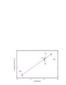
Figure 1: An expected signature of the time variation of the fine structure constant.

9 Current laboratory limitations

Current laboratory limitations are summarized in Table  5. A limitation on the time variation of the proton $g$ factor is derived assuming that the nuclear corrections to the Schmidt model are not important. That indeed cannot be considered as a reliable approach. All other limitations are obtained in a more reliable way. As was pointed out in $\!{}^{{\bf?}}$ (see also Table 3), the hyperfine interval in cesium is very difficult for interpretation because of significant nuclear corrections to the Schmidt model. Fortunately, it was demonstrated that there is no variation on a level of a part in $10^{15}$ per a year for a ratio of cesium-to-rubidium hyperfine structure $\!{}^{{\bf?}}$ (as a matter of fact that is the strongest laboratory limitation on a variation of a transition frequency). The hyperfine interval in the ground state of the rubidium-87 in contrast to cesium-133 can be sufficiently well described by its non-relativistic part with use of the Schmidt model for the nuclear magnetic moment $\!{}^{{\bf?}}$ (see also Table 3).

Table 5: Current limitations on a possible time variation of the fundamental constants.

Fundamental	Limitation for
constant	variation rate
$\alpha$	$1\times 10^{-14}$ yr-1
$m_{e}/m_{p}$	$2\times 10^{-13}$ yr-1
$\alpha^{2}\mu_{p}/mu_{e}$	$6\times 10^{-14}$ yr-1
$\alpha^{-3}\mu_{p}/mu_{e}$	$7\times 10^{-15}$ yr-1
$\mu_{p}/mu_{e}$	$2\times 10^{-14}$ yr-1
$g_{p}$	$4\times 10^{-16}$ yr-1
$\alpha^{2}\mu_{n}/mu_{e}$	$8\times 10^{-14}$ yr-1
$\mu_{n}/mu_{e}$	$6\times 10^{-14}$ yr-1
$g_{n}/g_{p}$	$5\times 10^{-14}$ yr-1

10 Precision spectroscopy: tests and reliability

Recent progress in frequency metrology delivered us a number of results, essentially more accurate than any previous data and the expected results can be even more accurate. In such a case we need to be sure that the results are reliable. In this section we briefly discuss possible tests of the accurate frequency measurements.

• The cesium hyperfine interval plays a special role in physics because of the definition of the second. It is realized in a number of laboratories and a comparison of different cesium standards is an important metrological work. The comparison shows that we have a sufficient understanding of the accuracy of cesium experiments (see e.g. $\!{}^{{\bf?}}$).

• Study of the ${}^{3}P_{1}-{}^{1}S_{0}$ transition in neutral calcium were performed independently at NIST $\!{}^{{\bf?}}$ and PTB $\!{}^{{\bf?}}$ and the results are consistent.

• Hyperfine structure of the ground state of ytterbium ion was measured independently at PTB and NML $\!{}^{{\bf?}}$. The results are consistent.

• An important approach to test systematic sources part by part may be a measurement of the isotopic shift and its comparison with theory. If theory is not accurate enough, there is still an option for a precision study. Theory is helpful to fix the form of dependence on the nuclear mass and the nuclear charge radius and the shape of the dependence may be checked via fitting.

• Similar test can be performed studying the hyperfine structure. E.g. a comparison of the $1s-2s$ transitions in hydrogen for different spin states $\!{}^{{\bf?}}$. Since the hyperfine splitting in the ground state is known with a high accuracy $\!{}^{{\bf?},{\bf?}}$, the comparison of the $1s-2s$ ultraviolet transitions yields us a value of the hyperfine interval in a metastable $2s$ state. The result is more accurate that one directly derived from a microwave measurement $\!{}^{{\bf?}}$ and in good agreement with theory $\!{}^{{\bf?}}$. The transitions under study $\!{}^{{\bf?}}$ as well as comparison with theory and early microwave measurements are summarized in Fig. 2.

         

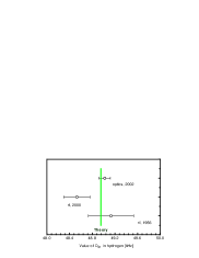
  Figure 2: Hyperfine structure in the hydrogen atom: levels scheme of an optical measurement of the $2s$ hfs interval and a comparison of theory to experiment for $D_{21}=8\times\nu_{\rm HFS}(2s)-\nu_{\rm HFS}(1s)$.

11 Summary

A comparison of different kinds of search for a possible time and space variations of the fundamental constants is summarized in Table 6. The characteristic level of the limitations is given suggesting a linear time dependence. In the case of oscillation the limitation from geochemical search and from astrophysical observations should be weakened by a factor $2\Delta t/T$, since the period of oscillation $T$ can be shorter than the time separation $\Delta t$. We note that in the case of laboratory limitation the results should depend on a current phase of oscillations. Another problem with interpretation of the astrophysical data is a separatation of space and time variations. The different kinds of search offer access to different sets of constants and their reliability depends on whether they are affected by the strong interactions.

Table 6: Comparison of different kind of search for a possible time and space variation of the fundamental constants.

	Geochemistry	Astrophysics	Laboratory	Laboratory
				(optics)
Drift or oscillation	$\Delta t\sim 10^{9}$ yr	$\Delta t\sim 10^{9}$ yr	$\Delta t\sim 1-30$ yr	$\Delta t\sim 1-10$ yr
Space variations	$\Delta l\simeq 10^{9}~{}c\times$yr	$\Delta l\simeq 10^{10}~{}c\times$yr	0	0
Level of limitations	$10^{-17}$ yr-1	$10^{-15}$ yr-1	$10^{-15}$ yr-1	$10^{-14}$ yr-1
Present results	Negative	Positive ($\alpha$)	Negative	Negative
Variation of $\alpha$	not reliable	accessible	accessible	accessible
Variation of $m_{e}/m_{p}$	not accessible	accessible	accessible	not accessible
Variation of $g_{p}$	not accessible	accessible	accessible	not accessible
Variation of $g_{n}$	not accessible	not accessible	accessible	not accessible
Strong interactions	not sensitive	not sensitive	sensitive	not sensitive

Despite a number of advantages and disadvantages of different approaches there is no favorite way. Since we have no background theory, we need to try as many searches as possible and as different as possible.

There are a number of problems which may be of interest and we’d like to attract attention to a few of them.

• A comparison of hyperfine intervals in the ground state of ⁸⁵Rb and ⁸⁷Rb allows to remove any variation of the fine structure constant due to atomic interactions and the frequency ratio is sensitive only to the proton $g$ factor via the Schmidt model and to strong interactions via corrections to the Schmidt model. Separation of atomic and nuclear physics can be helpful as a test measurement when a number of microwave intervals related to the hyperfine structure will be studied.

• Actual nuclear magnetic moments of ¹⁹⁹Hg and ¹⁷¹Yb are very close (the difference is below 5%) and their Schmidt values are the same (see Table 3). If that is a systematic effect, a comparison of the hyperfine intervals in these two ions can give a reliable result on a possible variation of the fine structure constant $\alpha$. We need better understanding of the magnetic moments of ¹⁹⁹Hg and ¹⁷¹Yb.

• Discussing different approaches, we need to mention an idea of $\!{}^{{\bf?}}$ to study a 3.5 eV nuclear transition in ²²⁹Th which lies in the optical domain. Its comparison with atomic transitions can have indeed no reliable interpretation, but the nuclear transition is very different from atomic transitions and may be sensitive to effects not detectable with other methods.

• Another approach related to the nuclear properties suggested $\!{}^{{\bf?}}$ precision studies of the nuclear magnetic moment with extremely small values, which are expected to be very sensitive to detuning of the fundamental constants. Indeed, it is not possible to measure a nuclear magnetic moment accurately enough. However, looking for their variations one can study the hyperfine structure of proper ions. As an example of an extremely small magnetic moment, let us mention ${}^{198}_{81}$Tl with a magnetic moment below $10^{-3}\;\mu_{N}$ ($T_{1/2}=5.3(5)$ h), ${}^{153}_{~{}62}$Sm ($\mu=-0.022\,\mu_{N}$, $T_{1/2}=46$ h) and ${}^{192}_{~{}79}$Au ($\mu=-0.009(2)\,\mu_{N}$, $T_{1/2}=4.9$ h) $\!{}^{{\bf?}}$. Understanding the nature of such small values is also necessary.

• One more question related to the subject: can we detect the expansion of the Universe in some laboratory experiments? The expansion leads to the red shift of the photons at a level of $10^{-10}$ yr^-1, however, there is no way to study a photon emitted a year ago in laboratory experiments. A chance can appear if we can use objects (planets, spacecrafts) at a distance related to $c\times(1-10)\;$min.

A search of a possible variation of the values of the fundamental constant presents a specific field involving both fundamental and applied physics. A search for new physics is based on frequency metrology providing a high motivation. The frequency metrology presents now limitations which are somewhat weaker than those from astrophysics but it has showed significant progress last years and it seems that higher accuracy of the laboratory measurements is just a matter of time and new results will be coming soon.

References

References

-
[1]
A. Linde, In Three Hundred Years of Gravitaion (Ed.
by S. W. Hawking and W. Israel, Cambridge University Press, Cambridge, 1987),
p. 604;
S. K. Blau and A. H. Guth, ibid., p. 524;
G. Börner, The Early Universe (Springer-Verlag, 1993). - [2] A. I. Shlyakhter, Nature (London) 264 (1976) 340. See also the preprints: A. I. Shlyakhter, LNPI N. 260 (1976); ATOMKI Report A/1 (1983).
- [3] S. G. Karshenboim, In Laser Physics at the Limits, ed. by H. Figger, D. Meschede and C. Zimmermann (Springer-Verlag, Berlin, Heidelberg, 2001), p. 165.
- [4] W. J. Marciano, Phys. Rev. Lett. 52, 489 (1984).
-
[5]
X. Calmet and H. Fritzsch, Eur. Phys. J. C24, 639 (2002);
H. Fritzsch: E-print hep-ph/0212186. - [6] J.-P. Uzan, E-print hep-ph/0205340.
- [7] K. Hagiwara et al., The Review of Particle Physics, Phys. Rev. D66, 010001 (2002).
- [8] P. A. M. Dirac, Nature 139 (1937) 323.
- [9] F. J. Dyson, In Aspects of Quantum Theory (Cambridge Univ. Press, Cambridge, 1972) p. 213; In Current Trends in the Theory of Fields (AIP, New York, 1983), p. 163.
- [10] S. G. Karshenboim, Can. J. Phys. 78, 639 (2000).
- [11] P. Langacker, G. Segre, and M. J. Strassler, Phys. Lett. B528, 121 (2002)
-
[12]
M. Maurette, Ann. Rev. Nucl. Part. Sci. 26, 319 (1972);
P. K. Kuroda, Origin of the Chemical Elements and the Oklo Phenomen (Springer-Verlag, Berlin, 1982). - [13] J. M. Irvine, Contemp. Phys. 24, 427 (1983).
- [14] T. Damour and F. Dyson, Nucl. Phys. B480, 596 (1994).
- [15] Y. Fujii, A. Iwamoto, T. Fukahori, T. Ohnuki, M. Nakagawa, H. Hidaka, Y. Oura, and P. Moller, Nucl.Phys. B573, 377 (2000).
- [16] J. K. Webb, M. T. Murphy, V. V. Flambaum, S. J. Curran, E-print astro-ph/0210531.
-
[17]
J. K. Webb, V. V. Flambaum, C. W. Churchill, M. J. Drinkwater, and J. D. Barrow, Phys. Rev. Lett. 82, 884 (1999);
J.K. Webb, M.T. Murphy, V.V. Flambaum, V.A. Dzuba, J.D. Barrow, C.W. Churchill, J.X. Prochaska, A.M. Wolfe, Phys. Rev. Lett. 87, 091301 (2001). - [18] A. Ivanchik, E. Rodriguez, P. Petitjean, and D. Varshalovich, Astron. Lett. 28, 423 (2002); A. Ivanchik, P. Petitjean, E. Rodriguez, and D. Varshalovich, E-print astro-ph/0210299.
- [19] H. Marion, F. Pereira Dos Santos, M. Abgrall, S. Zhang, Y. Sortais, S. Bize, I. Maksimovic, D. Calonico, J. Gruenert, C. Mandache, P. Lemonde, G. Santarelli, Ph. Laurent, A. Clairon, and C. Salomon: physics/0212112.
- [20] M. P. Savedoff, Nature 178, 688 (1956).
- [21] J. D. Prestage, R. L. Tjoelker, and L. Maleki, Phys. Rev. Lett. 74, 3511 (1995).
- [22] V. A. Dzuba, V. V. Flambaum, and J. K. Webb, Phys. Rev. A59, 230 (1999); V. A. Dzuba and V. V. Flambaum, Phys. Rev. A61, 034502 (2000).
- [23] R. I. Thompson, Astrophys. Lett. 16, 3 (1975).
-
[24]
H. B. G. Casimir, On the Interaction Between Atomic
Nuclei and Electrons (Freeman, San Francisco, 1963);
C. Schwarz, Phys. Rev. 97, 380 (1955). - [25] R. B. Firestone, Table of Isotopes (John Wiley & Sons, Inc., 1996).
- [26] M. Niering, R. Holzwarth, J. Reichert, P. Pokasov, Th. Udem, M. Weitz, T. W. Hänsch, P. Lemonde, G. Santarelli, M. Abgrall, P. Laurent, C. Salomon, and A. Clairon, Phys. Rev. Lett. 84, 5496 (2000).
- [27] G. Wilpers, T. Binnewies, C. Degenhardt, U. Sterr, J. Helmcke, and F. Riehle, Phys. Rev. Lett. 89, 230801 (2002).
- [28] J. von Zanthier; Th. Becker, M. Eichenseer, A. Yu. Nevsky, Ch. Schwedes, E. Peik, H. Walther, R. Holzwarth, J. Reichert, Th. Udem, T. W. Hänsch, P. V. Pokasov, M. N. Skvortsov, and S. N. Bagayev, Opt. Lett. 25 (2000) 1729.
- [29] J. Stenger, C. Tamm, N. Haverkamp, S. Weyers, and H. R. Telle, Opt. Lett. 26, 1589 (2001).
- [30] T. Udem, S. A. Diddams, K. R. Vogel, C. W. Oates, E. A. Curtis, W. D. Lee, W. M. Itano, R. E. Drullinger, J. C. Bergquist, and L. Hollberg, Phys. Rev. Lett. 86, 4996 (2001).
- [31] S. Bize, S. A. Diddams, U. Tanaka, C. E. Tanner, W. H. Oskay, R. E. Drullinger, T. E. Parker, T. P. Heavner, S. R. Jefferts, L. Hollberg, W. M. Itano, D. J. Wineland, and J. C. Bergquist, E-print physics/0212109.
-
[32]
T. Udem, J. Reichert, R. Holzwarth, S. Diddams, D. Jones, J. Ye, S. Cundiff, T. Hänsch, and J. Hall, In Hydrogen atom: Precision physics of simple atomic systems, ed by S. G. Karshenboim et al., (Springer, Berlin, Heidelberg, 2001), p. 125;
J. Reichert, M. Niering, R. Holzwarth, M. Weitz, Th. Udem, and T. W. Hänsch, Phys. Rev. Lett. 84, 3232 (2000);
R. Holzwarth, Th. Udem, T. W. Hänsch, J. C. Knight, W. J. Wadsworth, and P. St. J. Russell, Phys. Rev. Lett. 85, 2264 (2000);
S. A. Diddams, D. J. Jones, J. Ye, S. T. Cundiff, J. L. Hall, J. K. Ranka, R. S. Windeler, R. Holzwarth, Th. Udem, and T. W. Hänsch, Phys. Rev. Lett. 84, 5102 (2000). - [33] T. Parker, In Proceedings of the 6th Symposium Frequency Standards and Metrology, ed. by P. Gill (World Sci., 2002,) p. 89.
- [34] R. B. Warrington, P. T. H. Fisk, M. J. Wouters, and M. A. Lawn, In Proceedings of the 6th Symposium Frequency Standards and Metrology, ed. by P. Gill (World Sci., 2002), p. 297.
- [35] M. Fischer, N. Kolachevsky, S. G. Karshenboim and T.W. Hänsch, Can. J. Phys. 80, 1225 (2002); further analysis of systematic sources is in progress.
-
[36]
H. Hellwig, R.F.C. Vessot, M. W. Levine, P. W. Zitzewitz, D. W. Allan, and D. J. Glaze, IEEE Trans. IM 19, 200 (1970);
P. W. Zitzewitz, E. E. Uzgiris, and N. F. Ramsey, Rev. Sci. Instr. 41, 81 (1970);
D. Morris, Metrologia 7, 162 (1971);
L. Essen, R. W. Donaldson, E. G. Hope and M. J. Bangham, Metrologia 9, 128 (1973);
J. Vanier and R. Larouche, Metrologia 14, 31 (1976);
Y. M. Cheng, Y. L. Hua, C. B. Chen, J. H. Gao and W. Shen, IEEE Trans. IM 29, 316 (1980);
P. Petit, M. Desaintfuscien and C. Audoin, Metrologia 16, 7 (1980). - [37] N. E. Rothery and E. A. Hessels, Phys. Rev. A61, 044501 (2000).
- [38] S. G. Karshenboim and V. G. Ivanov, Phys. Lett. B524, 259 (2002); Euro. Phys. J. D19, 13 (2002).
- [39] E. Peik and Chr. Tamm, Europhys. Lett. 61, 181 (2003); E. Peik, contribution to this book.