Exact solutions of the equation governing the equilibrium magnetohydrodynamic states of an axisymmetric plasma with incompressible flows of arbitrary direction [H. Tasso and G.N. Throumoulopoulos, Phys. Pasmas 5, 2378 (1998)] are constructed for toroidal current density profiles peaked on the magnetic axis in connection with the ansatz $S=-ku$, where $S=d/du\left[\varrho(d\Phi/du)^{2}\right]$ ($k$ is a parameter, $u$ labels the magnetic surfaces; $\varrho(u)$ and $\Phi(u)$ are the density and the electrostatic potential, respectively). They pertain to either unbounded plasmas of astrophysical concern or bounded plasmas of arbitrary aspect ratio. For $k=0$, a case which includes flows parallel to the magnetic field, the solutions are expressed in terms of Kummer functions while for $k\neq 0$ in terms of Airy functions. On the basis of a tokamak solution with $k\neq 0$ describing a plasma surrounded by a perfectly conducted boundary of rectangular cross-section it turns out that the Shafranov shift is a decreasing function which can vanish for a positive value of $k$. This value is larger the smaller the aspect ratio of the configuration.

Published in Phys. Lett. A 317, 463-469 (2003)

1.  Introduction

Flow is a common phenomenon in astrophysical plasmas, in particular let us mention here the plasma jets that are observed to be spat out from certain galactic nuclei and propagate to supergalactic scales, e.g. Ref. [1]. Also, there has been established in fusion devices that sheared flow can reduce turbulence either in the edge region (L-H transition) or in the central region (internal transport barriers) thus resulting in a reduction of the outward particle and energy transport, e.g. Ref. [2].

In an attempt to contribute to the understanding of the equilibrium properties of flowing plasmas we considered cylindrical [3, 4], axisymmetric [5, 6], and helically symmetric [7] steady states with incompressible flows in the framework of ideal magnetohydrodynamics (MHD) by including the convective flow term in the momentum equation. Also we studied the equilibrium of a gravitating plasma with incompressible flow confined by a point-dipole magnetic field [8]. For an axisymmetric magnetically confined plasma the equilibrium satisfies [in cylindrical coordinates ($z,R,\phi$) and convenient units] the elliptic differential equation for the poloidal magnetic flux-function $\psi$,

$$(1-M_{p}^{2})\Delta^{\star}\psi-\frac{1}{2}(M_{p}^{2})^{\prime}|\nabla\psi|^{2}+\frac{1}{2}\left(\frac{X^{2}}{1-M_{p}^{2}}\right)^{\prime}+R^{2}\left(P_{s}\right)^{\prime}+\frac{R^{4}}{2}\left(\frac{\rho(\Phi^{\prime})^{2}}{1-M_{p}^{2}}\right)^{\prime}=0,$$ (1)

along with a Bernoulli relation for the pressure,

$$P=P_{s}(\psi)-\varrho\left[\frac{v^{2}}{2}-\frac{R^{2}(\Phi^{\prime})^{2}}{1-M_{p}^{2}}\right].$$ (2)

Here, $P_{s}(\psi)$, $\rho(\psi)$ and $\Phi(\psi)$ are, respectively, the static-equilibrium pressure, density and electrostatic potential which remain constant on magnetic surfaces $\psi(R,z)=\mbox{constant}$; the flux functions $F(\psi)$ and $X(\psi)$ are related to the poloidal flow and the toroidal magnetic field; $M_{p}=F^{\prime}/\sqrt{\varrho}$ is the Mach-number of the poloidal velocity with respect to the poloidal-magnetic-field Alfvén velocity; $\Delta^{\star}\equiv R^{2}\nabla\cdot(\nabla/R^{2})$; the prime denotes differentiation with respect to $\psi$. For vanishing flow (1) and (2) reduce to the Grad-Schlüter-Shafranov equation and $P=P_{s}(\psi)$, respectively. Derivation of (1) and (2) is given in Ref. [5]. It should be clarified that to simplify (22) of [5], the flux-function term $P_{s}-XF^{\prime}\Phi^{\prime}/(1-M^{2})$ therein has been replaced by $P_{s}$ in (1) here. Consequently, relation (19) of [5] for the pressure takes the form (2) here. Also, to emphasise that a poloidal-velocity Mach number is involved, $M$ in [5] is denoted by $M_{p}$ here.

Under the transformation

$$u(\psi)=\int_{0}^{\psi}\,[1-M_{p}^{2}(g)]^{1/2}\,d\,g,\ \ M_{p}^{2}<1,$$ (3)

(1) reduces to

$$\Delta^{\star}u+\frac{1}{2}\frac{d}{du}\left(\frac{X^{2}}{1-M_{p}^{2}}\right)+R^{2}\frac{dP_{s}}{du}+\frac{R^{4}}{2}\frac{d}{du}\left[\varrho\left(\frac{d\Phi}{du}\right)^{2}\right]=0.$$ (4)

The flow contributions here are connected with $M_{P}^{2}$ and $S\equiv d/du\left[\varrho\left(d\Phi/du\right)^{2}\right]$. Equation (4), free of the nonlinear term $1/2(M_{p}^{2})^{\prime}|\nabla\psi|^{2}$, can be analytically solved by assigning the $u$-dependence of the free flux functions $P_{s}$, $X$, $F$, $\varrho$, and $\Phi^{\prime}$. Relation (2) then determines the pressure. For $S=$ constant, exact solutions which extend the well known Solovév one were derived in Ref. [6]. Owing to the flow and its shear a variety of new configurations are possible having either one or two stagnation points in addition to the usual ones with a single magnetic axis.

The aim of the present work is to construct exact solutions of (4) for $S\propto u$ and examine their properties. The solutions are of the form (7) below in Section 2. This form is advantageous in that boundary conditions associated with either bounded laboratory plasmas or unbounded plasmas of astrophysical concern can be treated in a unified manner by adjusting appropriately the parameters it contains. As a matter of fact certain of the solutions we construct constitute extensions of the Hernegger-Maschke solution of the Grad-Schlüter-Shafranov equation for bounded plasmas [9, 10] and a recent one for unbounded plasmas derived by Bogoyavlenskij [11].

The work is organized as follows. Exact solutions of (4) for $S\propto u$ are constructed in Section 2. The flow impact on the Shafranov shift is then examined in Section 3 on the basis of a particular solution describing a tokamak configuration of arbitrary aspect ratio being contained within a perfectly conducting boundary of rectangular cross-section. Section 4 summarizes the Conclusions.

2.  Exact equilibrium solutions

Let us make the following particular choice for the free functions:

$$\frac{X^{2}}{1-M_{p}^{2}}=X_{0}^{2}+c_{1}^{2}u^{2},\ \ P_{s}=P_{s0}+2(-1)^{\gamma}c_{2}^{2}u^{2},\ \ \mbox{and}\ \ S\equiv\left[\rho(\Phi^{\prime})^{2}\right]^{\prime}=-64c_{3}c_{2}^{3}u.$$ (5)

under which (4) becomes linear. Here, the factor $(-1)^{\gamma}$ has been introduced in order to make comparison with solutions existing in the literature convenient, and $X_{0}$, $P_{s0}$, $c_{1}$, $c_{2}$, $c_{3}$ are constants. Equation (4) then takes the form

$$\Delta^{\star}u+c_{1}^{2}u+2(-1)^{\gamma}c_{2}xu-8c_{2}c_{3}x^{2}u=0,$$ (6)

where $x=2c_{2}R^{2}$. We pursue separable solutions of the form

$$u(R,z)=x^{n}P(x)T(z)\exp\left(-\frac{\gamma x}{2}\right).$$ (7)

This is appropriate for considering various equilibrium configurations in connection with different boundary conditions. In particular, the term $x^{n}$ which makes $u$ to vanish on the axis of symmetry is associated with either compact tori or spherical tokamak configurations. Plasmas surrounded by a fixed perfectly conducting boundary can be considered by setting $\gamma=0$. Unbounded plasmas are connected with $\gamma=1$, the exponential term guaranteeing smooth behaviour at large distances. It is noted that for static equilibria ($M_{p}=c_{3}=0$) the cases $n=\gamma=0$ and ($n=0,\gamma=1$) were considered in Refs. [9, 10], and [11], respectively.

With the use of (7) equation (6) leads to the following differential equations for $P(x)$ and $T(z)$:

$$T^{\prime\prime}+\omega^{2}T=0$$ (8)

and

$$xP^{\prime\prime}+(2n-\gamma x)P^{\prime}$$

$$+\left[\frac{4n(n-1)-4\gamma nx+\gamma^{2}x^{2}}{4x}+\frac{(-1)^{\gamma}x}{4}-\tau-c_{3}x^{2}\right]P=0,$$ (9)

where $\omega^{2}=$ constant and $\tau=(\omega^{2}-c_{1}^{2})/8c_{2}$. Therefore,

$$T(z)=A\sin(\omega z)+B\cos(\omega z)$$ (10)

and the problem additionally requires to solving (9). Solutions of (9) associated with different boundary conditions will be constructed in the subsequent subsections. It is noted here that all the solutions hold for arbitrary poloidal Mach numbers, viz. the dependence of $M_{p}^{2}(u)$ on $u$ remains free.

2.1  Unbounded plasmas ($\gamma=1$) and $c_{3}=0$

It is first noted that the case $c_{3}=0$ includes flows parallel to the magnetic field for $\Phi^{\prime}=0$, viz. when the electric field vanishes. For $c_{3}=0$, (1) becomes identical in form with the Grad-Schlüter-Shafranov equation and (9) reduces to

$$x^{2}P^{\prime\prime}+x(2n-x)P^{\prime}+\left[n(n-1)-(\tau+n)x\right]P=0.$$ (11)

Equation (11) can be solved by the following procedure. The substitution $P=x^{k}W(x)$, where $k$ is a root of the quadratic equation

$$k^{2}+(2n-1)k+n(n-1)=0,$$ (12)

leads to the following equation for $W(x)$:

$$xW^{\prime\prime}+[2(k+n)-x]W^{\prime}-(k+\tau+n)W=0.$$ (13)

The solutions of this equation can be expressed in terms of Kummer or confluent hypergeometric functions ([12], p. 503; [13], p. 137). In particular, for the two roots of (12) we have:

2.1.a   $k_{1}=-n$

The solution of (13) is

$$W(x)=x\left[D_{1}M(\tau+1,2,x)+D_{2}U(\tau+1,2,x)\right],$$

where $M$ and $U$ are the Kummer functions of first and second kind, respectively, and $D_{1}$, $D_{2}$ are constants. Consequently, the solution of the original equation (4) is written in the form

$$u(x,z) = x\left[D_{1}M(\tau+1,2,x)+D_{2}U(\tau+1,2,x)\right]\exp{\left(-x/2\right)}$$ (14)

$$\left[A\sin(\omega z)+B\cos(\omega z)\right].$$

For special values of $\tau$ and $n$ the Kummer functions reduce to simpler classical functions or polynomials (see Ref. [12], p. 509, table 13.6) ; in particular, for $\tau=-m$, where $m$ is a non-negative integer, and $n=0$ they reduce to Laguerre polynomials. Solutions of this kind for static equilibria ($M_{p}=0$) were derived in Ref. [11] and employed to model astrophysical jets and solar prominences. It may also be noted here that a continuation of this study and related studies were reported in Refs. [14, 15] and [16].

2.1.b   $k_{2}=-(n+1)$

The solutions of (13) and (4), respectively, read

$$W(x)=x^{3}\left[D_{1}M(\tau+2,4,x)+D_{2}U(\tau+2,4,x)\right],$$ (15)

and

$$u(x,z) = x^{2}[D_{1}M(\tau+2,4,x)+D_{2}U(\tau+2,4,x)]\exp{\left(-x/2\right)}$$ (16)

$$\left[A\sin(\omega z)+B\cos(\omega z)\right].$$

2.2   Bounded plasmas ($\gamma=0$) and $c_{3}=0$

Equation (9) then reduces to

$$x^{2}P^{\prime\prime}+2nxP^{\prime}+\left[n(n-1)-\tau x-\frac{1}{4}x^{2}\right]=0.$$ (17)

This equation can be solved by a procedure similar to that in Sec. 2.1, i.e the substitution $P=x^{k}W(x)$, where $k$ is again a root of (12), leads to

$$xW^{\prime\prime}+2(n+k)W^{\prime}-\left(\frac{1}{4}x+\tau\right)W=0.$$ (18)

Equation (18) has solutions of the form $W(x)=\exp(x/2)g(x)$. For the two roots of (12), $k_{1}=-n$ and $k_{2}=-(n+1)$ respectively, the solutions are

$$W(x)=\exp(x/2)\left[D_{1}M(-\tau,0,-x)+D_{2}U(-\tau,0,-x)\right],$$

and

$$W(x)=\exp(x/2)\left[D_{1}M(-(1+\tau),-2,-x)+D_{2}U(-(1+\tau),-2,-x)\right].$$

The respective solutions for $u(x,z)$ are

$$u(x,z)=\exp(x/2)\left[D_{1}M(-\tau,0,-x)+D_{2}U(-\tau,0,-x)\right]T(z)$$ (19)

and

$$u(x,z)=\exp(x/2)x^{-1}\left[D_{1}M(-(\tau+1),-2,-x)+D_{2}U(-(\tau+1),-2,-x)\right]T(z)$$ (20)

with $T(z)$ as given by (10).

As in Sec. 2.1, for special values of $\tau$ and $n$ the solutions of (17) can be expressed in terms of simpler classical functions or polynomials, e.g. for $n=0$ they are expressed in terms of Coulomb wave functions. In this case respective static solutions ($M_{p}=0$) were constructed in Refs. [9] and [10].

2.3  Bounded plasmas ($\gamma=0$) and $c_{3}\neq 0$

Changing independent variable by

$$\eta\equiv c_{3}^{-2/3}\left(c_{3}x-\frac{1}{4}\right),$$

(9) for $n=\tau=0$ is transformed into the Airy equation:

$$\frac{d^{2}P(\eta)}{d\eta^{2}}-\eta P(\eta)=0.$$ (21)

The general solution of (21) is

$$P(\eta)=d_{2}\left[B_{i}(\eta)+d_{1}A_{i}(\eta)\right]$$ (22)

where $A_{i}$ and $B_{i}$ are the Airy functions of first and second kind, respectively, and $d_{1}$ and $d_{2}$ are constants. An equilibrium symmetric with respect to the mid-plane $z=0$ then is described by

$$u=d_{2}\left[B_{i}(\eta)+d_{1}A_{i}(\eta)\right]\cos(c_{1}z).$$ (23)

For $c_{3}=0$, (23) takes the simpler form

$$u=d_{2}\left[\sin(\frac{x}{2})+d_{1}\cos(\frac{x}{2})\right]\cos(c_{1}z).$$

In next section solution (23) will be employed to evaluate the flow impact on the Shafranov shift.

In connection with solution (23) we now specify the plasma container to have rectangular cross-section of dimensions $a$ and $b$ and its geometric center to be located at $R_{0}$ (Fig. 1). Introducing the dimensionless quantities $\xi=R/R_{0}$, $\zeta=z/R_{0}$, $\lambda=c_{1}R_{0}$, $C=c_{2}R_{0}^{2}$, and

$$H=c_{3}^{-2/3}\left(2c_{3}C\xi^{2}-\frac{1}{4}\right)$$

(note that $c_{3}$ is dimensionless), we require that $u$ vanishes on the plasma boundary, viz.

$$u(H=H_{\pm})=u(\zeta=\pm\frac{a}{R_{0}})=0,$$

where

$$H_{\pm}=c_{3}^{-2/3}\left(2c_{3}{C}\xi_{\pm}^{2}-\frac{1}{4}\right)\ \ \mbox{and}\ \ \xi_{\pm}\equiv 1\pm\frac{b}{R_{0}}.$$

This requirement yields the eigenvalues

$$\lambda_{l}=\frac{R_{0}}{a}\left(l\pi+\frac{\pi}{2}\right),\ \ l=0,1,2,\ldots;\ \ {C}={C}_{k},\ \ k=1,2,\ldots$$

where ${C}_{k}$ can be determined by the equations

$$\frac{B_{i}(H_{k}^{+})}{A_{i}(H_{k}^{+})}=\frac{B_{i}(H_{k}^{-})}{A_{i}(H_{k}^{-})}=-D_{k},\ \ H_{k}^{\pm}=c^{-2/3}\left(2c_{3}C_{k}\xi_{\pm}^{2}-\frac{1}{4}\right).$$

The corresponding eigenfunctions normalized to a reference value $u_{c}$ are given by

$$\tilde{u}_{kl}=\frac{u_{kl}}{u_{c}}=\left[B_{i}(H_{k}(\xi)+D_{k}A_{i}(H_{k}(\xi))\right]\cos(\lambda_{l}\zeta).$$

The simplest eigenfunction corresponding to ($k=1$, $l=0$),

$$\tilde{u}_{10}=\frac{u_{10}(\xi,\zeta)}{u_{a}(\xi=\xi_{a},\zeta=0)}=\frac{\left[B_{i}(H_{1}(\xi))+D_{1}A_{i}(H_{1}(\xi))\right]\cos(\lambda_{0}\zeta)}{B_{i}(H_{1}(\xi_{a}))+D_{1}A_{i}(H_{1}(\xi_{a}))},$$ (24)

describes a configuration with a single magnetic axis located on $\zeta_{a}=0$ and $\xi=\xi_{a}=1+\Delta\xi$ with $\xi$ satisfying the equation

$$\frac{dB_{i}(H_{1}(\xi))}{d\xi}+D_{1}\frac{dA_{i}(H_{1}(\xi))}{d\xi}=0.$$ (25)

Here, $\Delta\xi$ is the Shafranov shift. Contours of constant $u$ and the Shafranov shift in connection with (24) are illustrated in Fig. 2.

For $c_{3}=0$ for which the functions $A_{i}$ and $B_{i}$ reduce to $\cos$ and $\sin$, respectively, the quantities $C_{k}$, $D_{k}$ and $\tilde{u}_{10}$ take the simpler forms: ${C}_{k}=R_{0}k\pi/(4b)$, $D_{k}=-\tan({C}_{k}\xi_{+}^{2})=-\tan({C}_{k}\xi_{-}^{2})$ and

$$\tilde{u}_{10}=\frac{u_{10}}{u_{c}}=\left[\sin({C}_{1}\xi^{2})+D_{1}\cos({C}_{1}\xi^{2})\right]\cos(\lambda_{0}\zeta).$$ (26)

The magnetic axis of the configuration described by (26) is located at ($\zeta=0,\xi=1+\sqrt{1+b^{2}/R_{0}^{2}}$).

The toroidal current density is given by

$$j_{\phi}=\left.\frac{\Delta^{\star}\psi}{R}=\frac{1}{R\left(1-M_{p}^{2}\right)^{1/2}}\left[\Delta^{\star}u+\frac{|\nabla u|^{2}}{2\left(1-M_{p}^{2}\right)}\frac{dM_{p}^{2}}{du}\right]\right|_{\mbox{\large u=u}_{10}}.$$

For Mach numbers of the form $M_{p}^{2}=u^{m}$, where $m>1$ the profile of $j_{\phi}$ is peaked on the magnetic axis and vanishes on the boundary.

On the basis of equation (25), $\Delta\xi$ has been determined numerically as a function of the flow parameter $c_{3}$ (Fig. 3). It is recalled that $c_{3}$ is related to the density and the electric field and their variation perpendicular to the magnetic surfaces by (5). As can be seen in Fig. 3, $\Delta\xi$ is a decreasing function of $c_{3}$ which goes down to zero sharply as $c_{3}$ approaches a positive value, this value being larger the smaller is the aspect ration $R_{0}/b$ of the configuration. This result is independent of the plasma elongation $a/b$. It is finally noted that suppression of the Shafranov shift by a properly shaped toroidal rotation profile was reported in Ref. [17].

We have constructed exact solutions of the equation describing the MHD equilibrium states of an axisymmetric magnetically confined plasma with incompressible flows [Eq. (4)] for $S=-ku$, where $S=d/du\left[\varrho(d\Phi/du)^{2}\right]$, corresponding to flows of arbitrary direction. The solutions are based on the form (7) which is convenient for applying boundary conditions associated with either unbounded plasmas or bounded ones. For $k=0$ the solutions are expressed in terms of Kummer functions [(Eqs. (14) and (16) for unbounded plasmas; (19) and (20) for bounded ones] while for $k\neq 0$ they are expressed in terms of Airy functions [Eq. (23)].

Solution (23) has then been employed to study a tokamak configuration of arbitrary aspect ratio being contained within a perfectly conducting boundary of rectangular cross-section and toroidal current density profile which can be peaked on the magnetic axis and vanish on the boundary. In this case it turns out that the Shafranov shift is a decreasing function of $k$ which can vanish for a positive value $k=k_{c}$, with $k_{c}$ being larger the smaller the aspect ratio of the configuration is. These results demonstrate that the shape of the density and the electric field profiles associated with flow and their variation perpendicular to the magnetic surfaces can result in a strong variation of the Shafranov shift.

Acknowledgements

Part of this work was conducted during a visit of one of the authors (GNT) to the Max-Planck Institut für Plasmaphysik, Garching. The hospitality of that Institute is greatly appreciated.

The present work was performed under the Contract of Association ERB 5005 CT 99 0100 between the European Atomic Energy Community and the Hellenic Republic.

Fig. 1  Boundary with rectangular cross-section in connection with the equilibrium solution (22).

Fig. 2.   The contours illustrate magnetic surface cross-sections in connection with solution (24) for two different values of the flow parameter $c_{3}$ which is related to the density and electric field and their variations perpendicular to the magnetic surfaces. The positions $\xi_{0}=1$ and $\xi_{a}$ refer to the geometric center and the magnetic axis, respectively. For $c_{3}=0.025$ the Shafranov shift $\Delta\xi=(R_{a}-R_{0})/R_{0}=\xi_{a}-\xi_{0}$ in Fig. 2b is drastically reduced in comparison with that for $c_{3}=0.005$ in Fig. 2a.

Fig. 3.  The Shafranov shift $\Delta\xi=(R_{a}-R_{0})/R_{0}$ versus the flow parameter $c_{3}$ for various values of the aspect ratio $R_{0}/b$. $\Delta\xi$ is determined numerically on the basis of (25) in connection with the equilibrium solution (24).

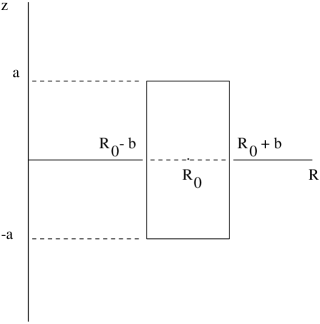
Figure 1: Boundary with rectangular cross-section in connection with the equilibrium solution (22).

\psfrag{z}{$\zeta$ \hskip 85.35826pt {\huge\cal 2a} \hskip 85.35826pt $c_{3}=0.005$}\psfrag{R}{$\xi$}\psfrag{R0}{$\xi_{0}$}\psfrag{Ra}{$\xi_{a}$}\includegraphics[scale={1}]{Fig24-2a.eps}

\psfrag{z}{$\zeta$ \hskip 85.35826pt {\huge\cal 2b} \hskip 85.35826pt $c_{3}$=0.025}\psfrag{R}{$\xi$}\psfrag{R0}{$\xi_{0}$}\psfrag{Ra}{$\xi_{a}$}\includegraphics[scale={1}]{Fig24-2b.eps}

Figure 2: The contours illustrate magnetic surface cross-sections in connection with solution (24) for two different values of the flow parameter $c_{3}$ which is related to the density and electric field and their variations perpendicular to the magnetic surfaces. The positions $\xi_{0}=1$ and $\xi_{a}$ refer to the geometric center and the magnetic axis, respectively. For $c_{3}=0.025$ the Shafranov shift $\Delta\xi=(R_{a}-R_{0})/R_{0}=\xi_{a}-\xi_{0}$ in Fig. 2b is drastically reduced in comparison with that for $c_{3}=0.005$ in Fig. 2a.

\psfrag{a}{$c_{3}$}\psfrag{b}{$\Delta\xi$}\psfrag{t1}{$R_{0}/b=1$}\psfrag{t2}{$R_{0}/b=2$}\psfrag{t3}{$R_{0}/b=4$ }\includegraphics[scale={1}]{Fig24-3.eps}

Figure 3: The Shafranov shift $\Delta\xi=(R_{a}-R_{0})/R_{0}$ versus the flow parameter $c_{3}$ for various values of the aspect ratio $R_{0}/b$. $\Delta\xi$ is determined numerically on the basis of (25) in connection with the equilibrium solution (24).

References

- [1] J. Eilek, Plasma Physics in Clusters of Galaxies, Review talk delivered in the 44th Plasma Physics Annual Meeting of the American Physical Society, Orlando, Florida, 11-15 November 2002; Bull. American Phys. Soc. 47, 18 (2002).
- [2] P. W. Terry, Rev. Mod. Phys. 72, 109 (2000).
- [3] G. N. Throumoulopoulos, G. Pantis, Plasma Phys. Contr. Fusion 38, 1817 (1996).
- [4] G. N. Throumoulopoulos, H. Tasso, Phys. Plasmas 4, 1492 (1997).
- [5] H. Tasso, G. N. Throumoulopoulos, Phys. Plasmas 5, 2378 (1998).
- [6] Ch. Simintzis, G. N. Throumoulopoulos, G. Pantis, H. Tasso, Phys. Plasmas 8, 2641 (2001).
- [7] G. N. Throumoulopoulos, H. Tasso, J. Plasma Physics 62, 449 (1999).
- [8] G. N. Throumoulopoulos, H. Tasso, Geophys. Astroph. Fluid Dynamics 94, 249 (2001).
- [9] F. Hernegger, Proceedings of the 5th EPS Conference on Controlled Fusion and Plasma Physics, Grenoble, 1972, edited by E. Canobbio et al. (Commissariat a l’Energie Atomique, Grenoble, 1972), Vol. I, p. 26.
- [10] E. K. Maschke, Plasma Phys. 15, 535 (1973).
- [11] O. I. Bogoyavlenskij, Phys. Rev. Lett. 84, 1914 (2000).
- [12] L. J. Slater, in Handbook of Mathematical Functions, edited by M. Abramowitz and I. A. Stegun, Dover Publications, 1964.
- [13] A. D. Polyanin, V. F. Zaitsev, Handbook of exact solutions for ordinary differential equations, CRC Press, 1995.
- [14] O. I. Bogoyavlenskij, Phys. Lett. A 276, 257 (2000).
- [15] O. I. Bogoyavlenskij, Phys. Lett. A 291, 256 (2001).
- [16] M. Núñez, Phys. Rev. E 67, 016403 (2003).
- [17] V. I. Il’gisonis, Yu. I. Pozdnyakov, JETP Letters 71, 314 (2000).
Figure captions