A Monte Carlo Calculation of the Pionium Break-up Probability with Different Sets of Pionium Target Cross Sections

Abstract

Chiral Perturbation Theory predicts the lifetime of pionium, a hydrogen-like $\pi^{+}\pi^{-}$ atom, to better than 3% precision. The goal of the DIRAC experiment at CERN is to obtain and check this value experimentally by measuring the break-up probability of pionium in a target. In order to accurately measure the lifetime one needs to know the relationship between the break-up probability and lifetime to a $1\%$ accuracy. We have obtained this dependence by modeling the evolution of pionic atoms in the target using Monte Carlo methods. The model relies on the computation of the pionium–target atom interaction cross sections. Three different sets of pionium–target cross sections with varying degrees of complexity were used: from the simplest first order Born approximation involving only the electrostatic interaction to a more advanced approach taking into account multi-photon exchanges and relativistic effects. We conclude that in order to obtain the pionium lifetime to 1% accuracy from the break-up probability, the pionium–target cross sections must be known with the same accuracy for the low excited bound states of the pionic atom. This result has been achieved, for low $Z$ targets, with the two most precise cross section sets. For large $Z$ targets only the set accounting for multiphoton exchange satisfies the condition.

1 Introduction

Pionium is the hydrogen-like electromagnetic bound state of a $\pi^{+}\pi^{-}$ pair. Its lifetime is determined by the strong $\pi^{+}\pi^{-}\rightarrow\pi^{0}\pi^{0}$ annihilation in the low relative momentum regime where Chiral Perturbation Theory applies. The theory predicts the pionium lifetime value of $(2.9\pm 0.1)\times 10^{-15}\mbox{ s}$ [1]. Experimentally, this value is being measured in a model-independent way by the DIRAC experiment at CERN [2].

Under the experimental conditions of DIRAC the pionic atoms are created in the inelastic scattering between $24\;\textrm{GeV}/c$ protons, supplied by the PS at CERN, and the nuclei of the target [3, 4], a chemically pure material of well-determined thickness.

A pionic atom propagating at relativistic speed inside the target interacts mainly electromagnetically with the target atoms. The electromagnetic cross section is on the order of a megabarn. These interactions can lead either to a transition between two bound states of pionium or to a dissociation (break-up). The scattering with the target atoms competes with the process of annihilation since a shorter pionium lifetime leads to a smaller break-up probability.

The main thrust of DIRAC’s experimental technique is the detection of $\pi^{+}\pi^{-}$ pairs with very low relative momentum. From the low-momentum part of the spectrum, the break-up probability of pionium is then determined.

The goal of this study is to establish the theoretical dependence of the break-up probability on the lifetime with a very high accuracy. We modeled the dynamics of pionium in different targets taking into account a large number of atomic shells that become populated as the pionic atom evolves in the target.

We have performed the calculations by using three sets of pionium target interaction cross sections. The original studies by Afanasyev and Tarasov [5] made use of the Born approximation and pure electrostatic interaction. In our work we have applied new corrected cross sections that take into account relativistic effects [6] and the multiphoton exchanges [9]. In addition, these cross section sets include a more accurate description of the target atomic form factor. As an error in the break-up probability translates directly to an error in lifetime, we have checked whether the results obtained in the new calculations significantly deviate from the previous ones. We conclude that the magnetic and relativistic corrections together with the target form factor choice are non-negligible mainly for the small $Z$ targets, whereas the multiphoton exchange should be considered for the large $Z$ ones.

2 Monte Carlo Simulation of Pionium in the Target

As we have noted in the introduction, to determine the pionium lifetime, the experiment DIRAC needs a precise theoretical calculation of the break-up probability $P_{\mathrm{br}}$ of pionium due to the electromagnetic interaction with target atoms. This calculation can be done by means of a Monte Carlo transport code that simulates the evolution of pionium from its creation to either its annihilation or its break-up under the given experimental conditions.

2.1 Pionium Production

The pionic atoms are formed as a consequence of the Coulomb final state interaction of two oppositely charged pions. These pions are created in an inelastic collision of a $24\;\textrm{GeV}/c$ proton and one of the target nuclei. The pionic atom is described by six quantities, accounting for the six degrees of freedom of a two body system. A particularly convenient choice of these quantities is given by the laboratory momentum of the center of mass of the atom $\vec{P}$ and the quantum numbers of the created bound state $n$, $l$, and $m$ in the spherical coordinate representation .

The probability of pionium being created is given by [3]

$$\frac{\rmd\sigma^{A}_{nlm}}{\rmd\vec{P}}=(2\pi)^{3}\left|\psi_{nlm}(0)\right|^{2}\vphantom{\Bigg{|}_{\vec{p}}}\frac{E}{M}\frac{\rmd\sigma^{0}_{s}}{\rmd\vec{p}\,\rmd\vec{q}}\Bigg{|}_{\vec{p}=\vec{q}=\vec{P}/2}.$$ (1)

The two terms on the right-hand side of the equation illustrate the final state interaction mechanism. The rightmost factor is the doubly inclusive cross section of $\pi^{+}$ and $\pi^{-}$ pairs at equal momenta ($\vec{p}=\vec{q}$) without considering the final state interaction, as indicated by the superscript $0$. The subscript $s$ means that only pions created from direct hadronic processes and decays of resonances with a very short lifetime are considered, because the Coulomb interaction of pions from long-lived sources (e.g. $\eta$, $K^{0}_{S}$ and $\Lambda$) is negligible and hence they do not contribute to pionic atoms production. The effect of the final state Coulomb interaction is to create a bound state with quantum numbers $n$, $l$, and $m$; it is given by the squared wave function at the origin.

The doubly inclusive cross section can be obtained from the direct measurements of time correlated $\pi^{+}\pi^{-}$ pairs in DIRAC, according to the following reasoning:

• The final state Coulomb interaction for short-lived sources is given, as in the case of the creation of a bound state, by a multiplicative factor depending only on $Q$, the magnitude of the relative momentum between the two pions. This is the so-called Coulomb or Gamow factor [11]

  $$\frac{\rmd\sigma_{s}}{\rmd\vec{p}\,\rmd\vec{q}}=A_{C}(Q)\frac{\rmd\sigma^{0}_{s}}{\rmd\vec{p}\,\rmd\vec{q}}\;;\qquad A_{C}(Q)=\frac{2\pi M_{\pi}\alpha/Q}{1-\rme^{-2\pi M_{\pi}\alpha/Q}}\;,$$ (2)

  where $\alpha$ is the fine structure constant.

• The contribution to the doubly inclusive cross section of pairs containing at least one pion from a long-lived source, $\omega_{l}(\vec{P})$, can be calculated with a hadron physics Monte Carlo simulation. In our case we have used FRITIOF6 [12]. This function has been shown to depend only on $P$ [15], the magnitude of the total momentum of the pion pair. Taking this into account together with (2) we find

  $$\frac{\rmd\sigma}{\rmd\vec{p}\,\rmd\vec{q}}=\frac{\rmd\sigma_{s}}{\rmd\vec{p}\,\rmd\vec{q}}+\frac{\rmd\sigma_{l}}{\rmd\vec{p}\,\rmd\vec{q}}=A_{C}(Q)\frac{\rmd\sigma_{s}^{0}}{\rmd\vec{p}\,\rmd\vec{q}}+\omega_{l}(P)\frac{\rmd\sigma}{\rmd\vec{p}\,\rmd\vec{q}}\;,$$ (3)

  thus relating $\sigma$ and $\sigma_{s}^{0}$.

• Finally, we have found that the $\vec{P}$-dependence of the doubly inclusive cross section is not correlated to $\vec{Q}$, given that $\vec{Q}\ll 30\;\textrm{MeV}/c$.

These findings allow us to relate the $\vec{P}$-dependence of $\sigma$ and $\sigma_{s}^{0}$ by

$$\left.\frac{\rmd\sigma^{0}_{s}}{\rmd\vec{p}\,\rmd\vec{q}}\right|_{\vec{p}=\vec{q}=\vec{P}/2}\propto\int_{0}^{Q\sim 2\;\mathrm{MeV}/c}(1-\omega_{l}(P))\frac{\rmd\sigma}{\rmd\vec{p}\,\rmd\vec{q}}\,\rmd\vec{Q}\;,$$ (4)

where the $\vec{P}$ distribution is obtained from the direct measurement of the laboratory momentum of low relative momentum $\pi^{+}\pi^{-}$ pairs in DIRAC. In figure 1 we show the distribution of the magnitude of the momentum $P$ and the angular distribution relative to the proton beam axis for low relative momentum $\pi^{+}\pi^{-}$ pairs.

The initial quantum number distribution depends on the value of the wave function at the origin. It has been shown [16] that the effect of the strong interaction between the two pions of the atom significantly modifies $|\psi_{nlm}(0)|$ in comparison to the pure Coulomb wave function. However, the ratio between the production rate in different states has been demonstrated to be kept as for the Coulomb wave functions [17]. Then, considering that the Coulomb functions obey

$$\left|\psi^{(\mathrm{C})}_{nlm}(0)\right|^{2}=\left\{\begin{array}[]{cl}0&\textrm{if $l\neq 0$,}\\ \displaystyle\frac{(\alpha M_{\pi}/2)^{3}}{\pi n^{3}}&\textrm{if $l=0$,}\end{array}\right.$$ (5)

we note that only $S$ states are created, according to a $1/n^{3}$ distribution.

Figure 1: The left graph shows the laboratory momentum magnitude distribution and the right graph the angular distribution with respect to the proton beam axis for low relative momentum $\pi^{+}\pi^{-}$ pairs.

Another quantity to be specified is the position where the proton–target interaction took place ($\vec{R}$). This is also the position where the atom was created. Since the target thickness is chosen much smaller than the nuclear interaction length of the target material, the $\pi^{+}\pi^{-}$ atoms are supposed to be uniformly generated all across the target thickness. The position in the transverse coordinates is unimportant, but it can be generated according to the beam profile characteristics, too.

We have now gathered all the information needed to simulate the creation of pionium atoms with a center of mass momentum $\vec{P}$ according to the experimentally measured momentum and angular distributions, at a position $\vec{R}$ uniformly distributed through the target, and in an initial $S$-wave state with the principal quantum number $n$ distributed according to a $1/n^{3}$ distribution.

2.2 Pionium Annihilation

Once an atom has been created in its initial state, specified by $\vec{P}$, $n$, $l$, and $m$, its dynamics are those of a free system that can either be annihilated, mainly via the $\pi^{+}\pi^{-}\rightarrow\pi^{0}\pi^{0}$ channel, or be electromagnetically scattered by one of the target atoms.

The strong interaction decay to two neutral pions determines the lifetime and is related to the $a_{0}^{0}-a_{0}^{2}$ scattering lengths difference and to the wave function at the origin by [18]

$$\frac{1}{\tau_{nlm}}=\frac{16\pi}{9}\frac{\sqrt{M_{\pi}^{2}-M_{\pi^{0}}^{2}-\frac{1}{4}M_{\pi}^{2}\,\alpha^{2}}}{M_{\pi}}(a_{0}^{0}-a_{0}^{2})^{2}(1+\delta_{\Gamma})\left|\psi^{(\mathrm{C})}_{nlm}(0)\right|^{2}\;,$$ (6)

where $M_{\pi}$ and $M_{\pi^{0}}$ are the masses of the charged and the neutral pion, respectively, and $\delta_{\Gamma}$ is the correction to next-to-leading order ($\delta_{\Gamma}=0.058$) that includes the effect of the strong interaction between the two pions. Using Chiral Perturbation Theory, Colangelo et al [1] have been able to calculate the most precise value of the scattering lengths difference to date ($a_{0}^{0}-a_{0}^{2}=0.265\pm 0.004$). Employing this value in (6) yields

$$\tau_{100}=(2.9\pm 0.1)\cdot 10^{-15}\;\textrm{s}.$$ (7)

Note, however, that due to (5) pionium may only decay from $S$ states. Moreover, the lifetime of any $S$ state is related to the lifetime of the ground state, by

$$\tau_{n00}=n^{3}\tau.$$ (8)

For the purpose of simulating pionium in the target, we shall from now on refer to $\tau$ as the pionium lifetime.

Hence, the probability for a $\pi^{+}\pi^{-}$ atom to annihilate per unit length, after the Lorentz boost transformation to the laboratory system, is given by

$$p_{nlm}^{\mathrm{anh}}=\frac{1}{\lambda_{nlm}^{\mathrm{anh}}}=\left\{\begin{array}[]{c@{\hspace{1cm}}l}\displaystyle\frac{2M_{\pi}}{Pn^{3}\tau}\hfil\hskip 28.45274pt&\textrm{if $l=0$,}\\ 0\hfil\hskip 28.45274pt&\textrm{other cases,}\end{array}\right.$$ (9)

where $\lambda_{nlm}^{\mathrm{anh}}$ is the annihilation mean free path.

2.3 Electromagnetic Interaction of Pionium with the Target

The electromagnetic pionium–target interaction of a pionic atom in an initial $nlm$ bound state can induce a transition to another $n^{\prime}l^{\prime}m^{\prime}$ bound state. The probability of such an interaction per unit length is given by

$$p_{nlm}^{n^{\prime}l^{\prime}m^{\prime}}=\frac{\rho N_{0}}{A}\sigma_{nlm}^{n^{\prime}l^{\prime}m^{\prime}}$$ (10)

where $\rho$ is the target density, $A$ its atomic weight, $N_{0}$ is the Avogadro number, and $\sigma_{nlm}^{n^{\prime}l^{\prime}m^{\prime}}$ are the discrete (bound–bound) transition cross sections.

The break-up mechanism is analogous to the discrete one; the break-up probability per unit length of an atomic bound state $nlm$ is given by

$$p_{nlm}^{\mathrm{br}}=\frac{1}{\lambda_{nlm}^{\mathrm{br}}}=\frac{\rho N_{0}}{A}\sigma_{nlm}^{\mathrm{br}}$$ (11)

where $\sigma_{nlm}^{\mathrm{br}}$ is the break-up (ionization) cross section.

Finally, the total cross section gives the probability of an atom to undergo an electromagnetic interaction and of course fulfills

$$\sigma_{nlm}^{\mathrm{em}}=\sum_{n^{\prime}l^{\prime}m^{\prime}}\sigma_{nlm}^{n^{\prime}l^{\prime}m^{\prime}}+\sigma_{nlm}^{\mathrm{br}}\;.$$ (12)

The total probability for a pionic atom to suffer an electromagnetic collision per unit length is then given by

$$p_{nlm}^{\mathrm{em}}=\frac{1}{\lambda_{nlm}^{\mathrm{em}}}=\frac{\rho N_{0}}{A}\sigma_{nlm}^{\mathrm{em}}\;,$$ (13)

where $\lambda_{nlm}^{\mathrm{em}}$ is the mean free path before an electromagnetic interaction takes place. Exploiting the completeness of the eigenstates of the Coulomb Hamiltonian the total electromagnetic cross sections can be calculated directly [19, 20] and not just via (12) .

The electromagnetic cross sections have been obtained with different approaches in [5, 6, 9]. We will devote section 5 to discussing the different break-up probabilities they lead to.

To get an insight into the magnitude of these interaction probabilities we show in figure 2 the average values of the annihilation, ionization, excitation and de-excitation probabilities per unit length. The average is taken over the even $z$-parity states (i.e., $l-m$ even) for fixed $n$. The atoms are created in even $z$-parity states ($l=m=0$) and the transitions to odd $z$-parity ones are strongly suppressed. The figure shows the probabilities using the coherent (interaction with the atom as a whole) contribution of the Born2 set of cross sections. This cross section set will be described in section 4. Any other choice among the cross section sets described in section 4 would lead to very similar results. The averages are defined as

$$\overline{p}_{n}^{\mathrm{anh}}=\displaystyle\frac{1}{n(n+1)/2}\sum_{lm}p_{nlm}^{\mathrm{anh}}\;,$$ (14)

$$\overline{p}_{n}^{\mathrm{br}}=\displaystyle\frac{1}{n(n+1)/2}\sum_{lm}p_{nlm}^{\mathrm{br}}\;,$$ (15)

$$\overline{p}_{n}^{n^{\prime}<n}=\displaystyle\frac{1}{n(n+1)/2}\sum_{lm}\sum_{n^{\prime}<n,l^{\prime}m^{\prime}}p_{nlm}^{n^{\prime}l^{\prime}m^{\prime}}\;,$$ (16)

$$\overline{p}_{n}^{n^{\prime}>n}=\displaystyle\frac{1}{n(n+1)/2}\sum_{lm}\left(p_{nlm}^{\mathrm{em}}-p_{nlm}^{\mathrm{br}}-\sum_{n^{\prime}\leq n,l^{\prime}m^{\prime}}p_{nlm}^{n^{\prime}l^{\prime}m^{\prime}}\right)\;,$$ (17)

where $n(n+1)/2$ is the number of even $z$-parity states for a given $n$.

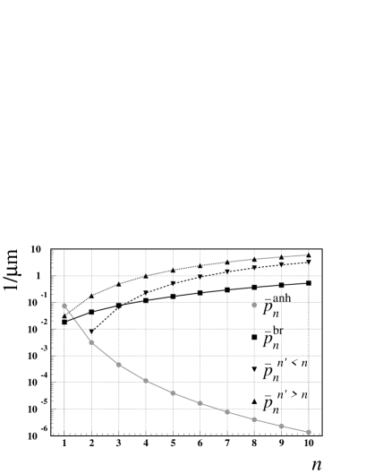
Figure 2: Annihilation, ionization, excitation and de-excitation probabilities per unit length, averaged over $l$ and $m$ quantum numbers according to equations (14), (15), (16) and (17), as a function of the principal quantum number $n$.

2.4 Pionium Evolution in the Target

To simulate the evolution of a pionic atom we use the following algorithm:

1. We generate a laboratory momentum $\vec{P}$, an initial set of quantum numbers and an initial position $\vec{R}$ for the atom as described in subsection 2.1.

2. We generate a free path according to:

   $$p(x)\,\rmd x=\frac{1}{\lambda_{nlm}}\rme^{-x/\lambda_{nlm}}\,\rmd x$$ (18)

   where $\lambda_{nlm}=(1/\lambda_{nlm}^{\mathrm{em}}+1/\lambda_{nlm}^{\mathrm{anh}})^{-1}$ is the mean free path before either an electromagnetic interaction or the annihilation takes place.

3. We displace the atom by the distance $x$:

   $$\vec{R}^{\prime}=x\frac{\vec{P}}{P}+\vec{R}.$$ (19)

4. We determine whether the atom has been annihilated, excited (or de-excited) in a discrete collision, or broken up. The relative weights of the respective branches of the evolution are given by the probabilities of equations (9), (10), and (11).

5. If the atom has been scattered and suffered a discrete transition we return to step (ii) using the new quantum numbers $n^{\prime}$, $l^{\prime}$ and $m^{\prime}$ and the new position $\vec{R}^{\prime}$ as the initial values.

More details on this model may be found in [21].

3 Break-up Probability Calculation

In principle, the break-up probability calculation of pionium should be straightforward once we have established the Monte Carlo model. The rest would be a matter of generating an atom sample and computing how many of them break up in the target. However, two main difficulties arise when trying to implement the algorithm.

The first difficulty is due to the presence of an infinite number of atomic bound states in the calculations. Clearly, only a finite number of states can be taken into account in the simulation of the evolution of pionium. In our calculations we have imposed a cut on the states with $n\leq n_{\max}$. This would not pose a serious problem if the atoms, being created mainly in very low $n$ states, could not get highly excited. Unfortunately, excitation to ever higher lying bound states constitutes a major branch in the evolution of pionium. As a consequence we cannot directly calculate the break-up probability as outlined in the previous paragraph.

The other difficulty lies in the fact that for some of the cross section sets to be studied in section 4, the break-up cross sections have not been calculated. In this case it is imperative to find an indirect way to compute the break-up probability.

We have discussed in the previous section that pionium terminates its evolution in the target by being either annihilated or broken up. However, the atom can also leave the target in a bound state. This would happen if one of the generated free paths in the Monte Carlo procedure carries it to a position outside the target. The break-up probability ($P_{\mathrm{br}}$), the annihilation probability ($P_{\mathrm{anh}}$), and the probability to leave the target in a discrete state ($P_{\mathrm{dsc}}$) are related by:

$$1=P_{\mathrm{br}}+P_{\mathrm{anh}}+P_{\mathrm{dsc}}\;.$$ (20)

This equation allows us to compute the break-up probability indirectly.

3.1 Computation Difficulties Due to Physical Characteristics of the Problem

The probability to generate an atom in a specific shell decreases as $1/n^{3}$. This means that the number of atoms created with $n\geq 4$ is very small. If the atoms could not get excited to states with large $n$, we could safely solve the evolution system by setting $n_{\max}>4$. However, as we saw in figure 2, the atoms have a tendency to be excited, as $n$ increases, rather than being annihilated or ionized.

Hence we expect a significant fraction of atoms excited into $n>n_{\max}$ shells even for large values of $n_{\max}$. The probability of an atom in a $nlm$ state to be excited into a state beyond the cut, i.e. with $n>n_{\max}$, is given by

$$p_{nlm}^{n^{\prime}>n_{\max}}=p_{nlm}^{\mathrm{em}}-p_{nlm}^{\mathrm{br}}-\sum_{n^{\prime}\leq n_{\max},\,l^{\prime}m^{\prime}}p_{nlm}^{n^{\prime}l^{\prime}m^{\prime}}$$ (21)

where we have used (10), (11) and (13). However, once the atom jumps into one of these states we loose control over it and we have to stop its evolution.

To analyze the change of the Monte Carlo results with $n_{\max}$ we have modeled the evolution of a sample of atoms by changing $n_{\max}$ from 7 to 9. We observed three main effects:

• The fraction of annihilated atoms ($P_{\mathrm{anh}}(n\leq n_{\max})$) does not change significantly.

• The portion of atoms leaving the target in discrete states ($P_{\mathrm{dsc}}(n\leq n_{\max})$) changes only slightly.

• The fraction of dissociated atoms ($P_{\mathrm{br}}(n\leq n_{\max})$) changes significantly.

This effect can be understood by checking the dependence of the annihilation, the discrete and the break-up probabilities on $n$, the principal quantum number of the state from which the atom was annihilated, broken-up, or in which it left the target. In figure 3 we show the result of the Monte-Carlo simulation with $n_{\max}=8$ for a sample of one million atoms using the Born2 cross section set that also includes cross sections for the ionization (refer to section 4). For the annihilated atoms we can see that $P_{\mathrm{anh}}(n)$ is negligible for values of $n\gtrsim 4$. The $P_{\mathrm{dsc}}(n)$ dependence also shows a fast, but less drastic, decrease with $n$. Only the solution for the states with $n=n_{\max}-1$ or $n=n_{\max}-2$ is unstable under variation of $n_{\max}$. For $n_{\max}=8$ this is a small contribution to the total $P_{\mathrm{dsc}}$ value. Finally, $P_{\mathrm{br}}(n)$ decreases very slowly with $n$, showing that there is a significant fraction of atoms broken up from states with $n>n_{\max}$. The probability of an atom to be excited into such a state with $n>n_{\max}$ is also shown as a function of the principal quantum number of the last state before the excitation. Obviously, this effect is non-negligible.

Figure 3: Probabilities of finishing the evolution in a discrete state (a), by annihilation (b), or by ionization (c) as a function of the parent state’s principal quantum number. In (d) we show the probability for an atom in an state $n$ to be excited into a non-controlled state with $n>8$. The results are for pionium in a $95\;\mu$m Ni target and the lifetime is assumed to be $3\cdot 10^{-15}$ s.

For the cross section sets without break-up cross sections, we can calculate directly only the total probability for all electromagnetic processes and the probabilities for discrete transitions to states with $n^{\prime}<n_{\max}$. In these cases we can therefore not distinguish whether an atom has been broken up or excited into a state with $n^{\prime}>n_{\max}$, that is, we can only determine the combination of probabilities

$$p_{nlm}^{n^{\prime}>n_{\max}}+p_{nlm}^{\mathrm{br}}=p_{nlm}^{\mathrm{em}}-\sum_{n^{\prime}\leq n_{\max},\,l^{\prime}m^{\prime}}p_{nlm}^{n^{\prime}l^{\prime}m^{\prime}}.$$ (22)

This is, of course, equivalent to (21), but in this case $p_{nlm}^{\mathrm{br}}$ is unknown. Thus, for these cross section sets not even the break-up probability for low $n$ states could be directly calculated and we are forced to use the procedure described below.

3.2 Calculation Procedure

Based on the fast decrease of $P_{\mathrm{anh}}$ and $P_{\mathrm{dsc}}$ as a function of $n$ we can assume that almost every atom excited to a state $n>n_{\max}$ will be eventually broken up. This will be true even though the excitation probability per unit length of a given bound state is significantly larger than the break-up probability per unit length. We can explain it as follows. The mean free path of the excited atoms strongly decreases with increasing $n$. For $n\sim 8$ the mean free path is $\lesssim 0.1\;\mu$m. An excited atom will thus interact many times within a very short distance. In every scattering the atom will have some small probability to break up, thereby terminating its evolution. In summary, the most probable evolution of an atom that has been excited to any state with $n\gtrsim 4$ is a sequence of excitations (and less frequent de-excitations) terminated by break-up.

However, while we are neglecting the atomic annihilation from states with $n>8$ and thus setting $P_{\mathrm{anh}}=P_{\mathrm{anh}}(n\leq 8)$, we can estimate $P_{\mathrm{dsc}}(n>8)$ by means of a fit to the $P_{\mathrm{dsc}}(n)$ histogram as recommended in [5]

$$P_{\mathrm{dsc}}(n>8)=\frac{a}{n^{3}}+\frac{b}{n^{5}}.$$ (23)

Hence, taking into account (20) we obtain

$$P_{\mathrm{br}}=1-P_{\mathrm{dsc}}-P_{\mathrm{anh}},$$ (24)

where $P_{\mathrm{dsc}}$ consists of two parts,

$$P_{\mathrm{dsc}}=P_{\mathrm{dsc}}(n\leq 8)+P_{\mathrm{dsc}}(n>8),$$ (25)

of which $P_{\mathrm{dsc}}(n\leq 8)$ is computed directly and $P_{\mathrm{dsc}}(n>8)$ is calculated from (23). In this manner we can calculate the break-up probability even without ionization cross sections as input.

In table 1 and in figure 4 (top left) we show a few results for the probability for different lifetime values in a $95\;\mu$m Ni target. The target choice coincides with that of the DIRAC experiment. We observe that the result of $P_{\mathrm{dsc}}(n>8)$ adds only a small correction. In figure 4 we also show the ionization and annihilation distributions as a function of the target position, and finally the creation position for those atoms that managed to emerge from the target in a bound state. As emphasized in subsection 3.1, with increasing $n$ only the atoms very near the target end will be able to leave the target in a discrete state.

Table 1: Results for the different probabilities defined in (20), as calculated with the Born2 cross section set for a sample of ten million pionic atoms in a $95\;\mu$m thick Nickel target.

$\tau[10^{-15}\;\textrm{s}]$	$P_{\mathrm{br}}$	$P_{\mathrm{anh}}$	$P_{\mathrm{dsc}}(n\leq 8)$	$P_{\mathrm{dsc}}(n>8)$
1	0.2976	0.6527	0.0491	0.0006
2	0.3951	0.5287	0.0754	0.0008
3	0.4599	0.4451	0.0941	0.0009
4	0.5062	0.3848	0.1080	0.0010
5	0.5408	0.3392	0.1190	0.0010
6	0.5681	0.3029	0.1279	0.0011
7	0.5901	0.2740	0.1348	0.0011

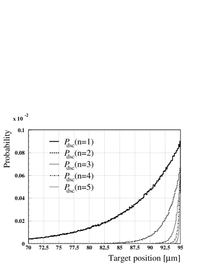
Figure 4: Top left: The break-up, annihilation, and discrete probabilities as a function of lifetime. Top right: Break-up and annihilation position distributions. Bottom: Creation position of those atoms that leave the target in a bound state (and contribute to $P_{\mathrm{dsc}}$). Note that as $n$ increases, only the atoms very near the target end can escape from it. All three plots refer to a $95\;\mu$m Ni target. In the last two, the lifetime is assumed to be $3\cdot 10^{-15}$ s.

4 Cross Sections Sets

In our calculations of the break-up probability we employed three different sets of cross sections. The first two have been calculated in the framework of the Born approximation. We assign the labels Born1 to the calculations made in reference [5] and Born2 to those of [6]. The two sets differ in four main points:

• The Born1 set neglects the contribution of incoherent scattering (collisions leading to an excitation of the target atom), thus considering the coherent interaction only (collisions with the target atom as a whole), i.e. the leading term. By contrast the Born2 set accounts for target excitations.

• The Born1 set uses Molière’s parameterization [22] for the Thomas-Fermi equation solution as the target atom form factor of the pure electric interaction, whereas the Born2 set takes electron orbitals determined numerically within the Hartree-Fock framework for the same purpose. The Thomas-Fermi-Molière parameterization of the atomic form factor is accurate for low momentum exchange, but gives a small excess for harder scattering.

• The Born1 set considers the sudden approximation (no recoil energy for the target and the pionic atom) and neglects the energy difference between the initial and the final state, while the Born2 set accounts for these two effects.

• Finally, Born2 set also considers the effect of magnetic and relativistic terms.

In principle it has been concluded [6] that accounting for second order effects like the magnetic terms of the Hamiltonian, the recoil energy of the atoms, or the relativistic terms generally leads to an overall decrease of the sudden approximation pure electrostatic coherent cross section value due to destructive interference with the leading orders. Moreover, employing atomic orbitals obtained in the Hartree-Fock approach for the form factor used to compute these cross sections leads to lower values than those of the Born1 set since the Molière parameterization of the solution to the Thomas-Fermi equation is excessive for mean and large values of the photon momentum transfer. This last issue leads to discrepancies that increase for large $n$ states and decrease for large $Z$ target atoms. The difference appears to be balanced by neglecting the incoherent contribution to the cross section in the Born1. This results in a systematically smaller ground state cross section of Born1 set whereas for larger $n$ Born1 cross sections are larger (up to $\sim 10\%$ discrepancy) or compatible with Born2 results. We can observe the comparison for three target materials in figure 5 and we shall analyze the disagreement in the break-up probability resulting from this effect.

Figure 5: In the left column we compare the Born1 and Born2 cross section sets. The middle column shows a comparison of the Born1 and Glauber sets and finally on the right we compare the Born2 and Glauber sets. The comparison is made for Titanium ($Z=22$), Nickel ($Z=28$) and Platinum ($Z=78$). The plots refer to total electromagnetic cross sections averaged over $m$ for even $z$-parity states.

Finally we have also used a set of cross sections where the Glauber formalism has been applied to calculate the coherent contribution to the cross section value. The details are given in [9]. This calculation technique accounts for multi-photon exchange in the pionium–target atom collision. Contrary to what one would expect the consideration of more than one photon being exchanged diminishes the values of the cross sections due to a destructive interference of the $n$-photon exchange contributions (this happened also when accounting for magnetic terms in the Born2 set). The leading order of the Glauber result matches the sudden approximation of the Born cross sections (since both neglect the difference between the initial and the final state energies). However, this cross section set uses a parameterization for the target atom form factors similar to the ones used in Born2. This explains the disagreement with respect to the Born1 and the agreement with Born2 set for low $Z$ targets, as can be seen in figure 5. The corrections due to multiphoton exchange are important for large $Z$ targets [9] and this explains the large discrepancies obtained for Platinum.

5 Results and Conclusions

After the discussions of the previous sections, we finally present the results of the break-up probability calculation. The DIRAC experiment has the possibility of choosing between several targets. The design of these different targets has been made to achieve the maximum break-up probability resolution in different lifetime ranges. Large $Z$ targets with larger interaction cross sections are better suited for small lifetime values whereas lower $Z$ materials are more sensitive to larger lifetime values. Three of these targets are the Pt $28\;\mu$m target, suitable for lifetime ranges $\tau<1\cdot 10^{-15}\;$s, the Ni $95\;\mu$m target for $\tau\sim 3\cdot 10^{-15}\;$s and the Ti $251\;\mu$m target for $\tau\sim 4\cdot 10^{-15}\;$s. The target thickness was chosen so as to have the same radiation length and hence equivalent multiple scattering effects for all three targets. The Nickel target constitutes DIRAC’s main target with which 90% of the data have been collected, as it is optimal for the theoretically predicted lifetime value.

In figure 6 the break-up probability curves are shown for these three targets. The calculation has been carried out for samples of ten million events, with a statistical error less than $0.08\%$.

One can clearly see that for the Ti and Ni targets the Glauber and Born2 sets lead to similar results whereas the Born1 set shows a $\sim 8\%$ disagreement. For the large $Z$ target (Pt) both Born1 and Born2 are biased toward large values. In this case, the multi-photon contributions to the total cross sections are not negligible. In any case the discrepancies between the break-up probability results are at the level of the discrepancies between ground state cross sections and much smaller than the differences between cross sections sets for medium or highly excited states. We can understand this based on the fact that the probability for the atoms to leave the target in a discrete state other than the ground state and maybe the first excited shell $P_{\mathrm{dsc}}(n\gtrsim 2)$ is of the order of, or smaller than, 5%. Hence, even large uncertainties in this magnitude (up to $10-15\%$) lead to very small changes in the break-up probability result. Only discrepancies in the ground state population and maybe the first excited shell, where most of the atoms are created, would lead to significant differences between the break-up probability results of the different sets.

Graphically we can view the atom as a balloon being inflated in every collision with the target. The different sets will lead to similar results of the size increase rate as long as the atom remains in a low excited state. However, as the atom grows (inflates) it will no longer be able to advance as easily in the target due to its large size and will finally break-up (explode). Large discrepancies in the excitation and break-up rate of the excited atom will not be important given that the mean free paths for the excited states are very small compared to the target dimensions.

In summary, we recall that the high precision measurement attempted by the DIRAC collaboration also requires an accuracy to better than $1\%$ in our theoretical break-up probability calculations. We note that the seemingly large discrepancies among our different cross section sets particularly for pionium transitions starting from highly excited states do not lead to significant differences in the theoretical break-up probabilities. The discrepancies between break-up probabilities are coming almost entirely from differences in the cross sections for the lowest lying states, where both the atomic structure of the target and the multi-photon transitions need to be treated as accurately as possible. This challenge, however, has already been mastered in our previous works [6, 20] where we showed that the required 1% accuracy can be achieved with our calculations, albeit only with the Born2 and the Glauber sets for low $Z$ and with the Glauber set for large $Z$ targets. The important conclusion of the present investigation is the finding that the (infinitely many!) highly excited states of pionium do not limit the validity of our approach even though we can include explicitly only a moderate number of these states in our simulations.

Figure 6: The break-up probability results for the three cross section sets and the three target materials.

Table 2: Comparison of the break-up probability results for the Ti $251\;\mu$m, the Ni $95\;\mu$m and the Pt $28\;\mu$m targets. The lifetime value is assumed to be $3\cdot 10^{-15}\;$s in the calculations.

Target	$P_{\mathrm{br}}^{\mathit{Born1}}$	$P_{\mathrm{br}}^{\mathit{Born2}}$	$P_{\mathrm{br}}^{\mathit{Glauber}}$	$1-\displaystyle\frac{P_{\mathrm{br}}^{\mathit{Born2}}}{P_{\mathrm{br}}^{\mathit{Born1}}}$	$1-\displaystyle\frac{P_{\mathrm{br}}^{\mathit{Glauber}}}{P_{\mathrm{br}}^{\mathit{Born1}}}$	$1-\displaystyle\frac{P_{\mathrm{br}}^{\mathit{Glauber}}}{P_{\mathrm{br}}^{\mathit{Born2}}}$
Ti	0.3026	0.3249	0.3232	$-7.4\%$	$-6.8\%$	$0.5\%$
Ni	0.4425	0.4599	0.4555	$-3.9\%$	$-2.9\%$	$1.0\%$
Pt	0.7137	0.7196	0.6924	$-0.8\%$	$3.0\%$	$3.8\%$

References

References

- [1] Colangelo G, Gasser J and Leutwyler H 2000 Phys. Lett.B 488 261.
- [2] Adeva B et al1995 Lifetime measurement of atoms to test low energy QCD predictions CERN/SPSLC 95-1 (Geneva: CERN); http://www.cern.ch/DIRAC
- [3] Nemenov L L 1985 Sov. J. Nucl. Phys. 41 629.
- [4] Gortchakov O E, Kuptsov A V, Nemenov L L and Riabkov D Yu 1996 Phys. of At. Nucl. 59 2015.
- [5] Afanasyev L G and Tarasov A V 1996 Phys. of At. Nucl. 59 2130.
- [6] Halabuka Z, Heim T A, Trautmann D and Baur G 1999 Nucl. Phys.554 86.
- [7] [] Heim T A, Hencken K, Trautmann D and Baur G 2000 J. Phys. B: At. Mol. Opt. Phys.33 3583.
- [8] [] Heim T A, Hencken K, Trautmann D and Baur G 2001 J. Phys. B: At. Mol. Opt. Phys.34 3763.
- [9] Schumann M, Heim T A, Hencken K, Trautmann D and Baur G 2002 J. Phys. B: At. Mol. Opt. Phys.35 2683.
- [10] Afanasyev L G, Jabitski M, Tarasov A and Voskresenskaya O 1999 Proc. of the Workshop HadAtom99 (Bern) hep-ph/9911339 p 14.
- [11] Landau L D and Lifshitz E M 1976 Quantum Mechanics (Non-Relativistic Theory) 3rd edition, Pergamon Press.
- [12] Uzhinskii V V 1996 JINR preprint E2-96192 Dubna.
- [13] [] Andersson B et al1987 Nucl. Phys.B 281 289.
- [14] [] Nilsson-Almquist B and Stenlund E 1987 Comp. Phys. Comm 43 387.
- [15] Afanasyev L G et al1997 Phys. At. Nucl. 60 938.
- [16] Kuraev E A 1998 Phys. of At. Nucl. 61 239.
- [17] Amirkhanov I, Puzynin I, Tarasov A, Voskresenskaya O and Zeinalova O 1999 Phys. Lett.B 452 155.
- [18] Gasser J, Lyubovitskij V E and Rusetsky A 1999 Phys. Lett.B 471 244.
- [19] Mrówczyński S 1987 Phys. Rev.D 36 1520.
- [20] Afanasyev L G, Tarasov A V and Voskrenskaya O O 1999 J. Phys. G: Nucl. Part. Phys.25 B7.
- [21] Santamarina C 2001 Detección e medida do tempo de vida media do pionium no experimento DIRAC Ph. D. Thesis, Universidade de Santiago de Compostela.
- [22] Molière G 1947 Z. Naturforsch. 2a 133.