Island Resonances

Abstract

Resonances driven by the error field multipoles in the magnets often show themselves as islands in phase plots of the particle motion. In order to be able to measure the strength of the island resonance, and then to correct it, it is helpful to study how these resonances show themselves. In particular , one can study how the presence of the island resonances distort the tune dependence on the amplitude, and the emittance growth caused by the island resonance. Islands in 4-dimensional phase space, unlike islands in 2-dimensional phase space, are not easy to visualize. This study will show how to visualize the islands in 4-dimensional phase space by studying the tune dependence on the amplitude of the particle. These effects are to some extent measureable, and can lead to a way to correct the resonance.

Introduction

Resonances driven by the error field multipoles often show themselves as islands in phase plots of the particle motion. This happens when there is another non-linear field present, besides the error field multipoles, which produces a strong enough dependence of the tune on the amplitude of the particle motion. Non-linear fields that produce a dependence of the tune on the ampliude can be the quadrupole fringe field , space charge fields and octupole correctors. In some cases it may be advantageous to introduce a non-linear field that produces a dependence of the tune on the amplitude of the particle motion. In order to be able to measure the strength of the island resonance, and then to correct it, it is helpful to study how these resonances show themselves. In particular , one can study how the presence of the island resonances distort the tune dependence on the amplitude and the emittance growth caused by the island resonance. These effects are to some extent measureable, and can lead to a way to correct the resonance. Islands in 4-dimensional phase space, unlike islands in 2-dimensional phase space, are not easy to visualize. This study will show how to visualize the islands in 4-dimensional phase space by studying the tune dependence on the amplitude of the particle. Again, this effect is to some extent measureable, and can lead to a way to measure the strength of the resonance.

Figure 1: $p_{x}$ vs. $x$ for the $3\nu_{x}=19$ resonance excited by a random $b_{2}$ in the SNS magnets. The initial coordinates have $x_{0}=24mm$ to $x_{0}=44mm$ in steps of 2 mm with $p_{x0}=0$ and $\epsilon_{y}=0$ .$\nu_{x0}=6.3267,\nu_{y0}=6.2267$. In the figure $x0,px0,y0,py0,epx0,ept0,nux0,nuy0$ represent $x_{0},p_{x0},y_{0},p_{y0},\epsilon_{x0},\epsilon_{y0},\epsilon_{t0},\nu_{x0},\nu_{y0}$.

Figure 2: $\nu_{x}$ versus $\epsilon_{x0}$ for the $3\nu_{x}=19$ resonance excited by a random $b_{2}$ in the SNS magnets. The initial coordinates have $x_{0}=24mm$ to $x_{0}=44mm$ in steps of 2 mm with $p_{x0}=0$ and $\epsilon_{y0}=0$ .$\nu_{x0}=6.3267,\nu_{y0}=6.2267$. In the figure $x0,px0,y0,py0,epx0,ept0,nux0,nuy0$ represent $x_{0},p_{x0},y_{0},p_{y0},\epsilon_{x0},\epsilon_{y0},\epsilon_{t0},\nu_{x0},\nu_{y0}$.

Figure 3: $d\epsilon_{x,max}$ vs $\epsilon_{x0}$ for the $3\nu_{x}=19$ resonance excited by a random $b_{2}$ in the SNS magnets. The initial coordinates $x_{0},p_{x0}$ lie along the direction in $x_{0},p_{x0}$ phase space given by $p_{x0}=0$ and $\epsilon_{y}=0$. $\nu_{x0}=6.3267,\nu_{y0}=6.2267$. In the figure $x0,px0,y0,py0,epx0,ept0,nux0,nuy0$ represent $x_{0},p_{x0},y_{0},p_{y0},\epsilon_{x0},\epsilon_{y0},\epsilon_{y0},\epsilon_{t0},\nu_{x0},\nu_{y0}$.

Figure 4: $d\epsilon_{x,max}$ vs $\nu_{x}$ for the $3\nu_{x}=19$ resonance excited by a random $b_{2}$ in the SNS magnets. The initial coordinates $x_{0},p_{x0}$ lie along the direction in $x_{0},p_{x0}$ phase space given by $p_{x0}=0$ and $\epsilon_{y0}=0$. $\nu_{x0}=6.3267,\nu_{y0}=6.2267$. In the figure x0,px0,y0,py0,epx0,ept0,nux0,nuy0 represent $x_{0},p_{x0},y_{0},p_{y0},\epsilon_{x0},\epsilon_{y0},\epsilon_{t0},\nu_{x0},\nu_{y0}$.

Resonances in 2-dimenional phase space

This section will study an island resonance in 2-dimensional phase space, the $3\nu_{x}=19$ resonance in the storage ring of the SNS (Spallation Neutron Source at Oak Ridge). This resonance is driven by the random error sextupole, $b_{2}$, in the magnets. In the absence of space charge forces, a non-linear field that produces an appreciable tune dependence on the amplitude of the particle motion is provided by the fringe field of the quadrupoles [1], which causes the tune to increase with the amplitude . Starting with a zero amplitude tune of $\nu_{x}=6.3267$ , $3\nu_{x}=19-.02$, one finds the phase space plot shown in Fig. 1. This plot was generated starting with $x_{0}=24mm$, $p_{x_{0}}=0$ and then increasing $x_{0}$ in steps of 2 mm keeping $p_{x_{0}}=0$ and tracking the particle for 1000 turns for each $x_{0}$. The tune starts below the resonance, and increases with amplitude. The islands appear when the tune reaches $\nu_{x}=6.3333$. The islands are reached when the initial amplitude is increased to $x_{0}=30mm$, $p_{x_{0}}=0$, which corresponds to an initial horizontal emittance of about $\epsilon_{x0}=115$ mm.mrad.

The distortion of the tune dependence on amplitude is shown in Fig. 2 where the horizontal tune is plotted against $\epsilon_{x0}$. Fig. 2 is generated by doing a search along the $p_{x_{0}}=0$ direction, increasing $x_{0}$ in steps of 2 mm. Fig. 2 shows a flat region where $\nu_{x}=6.3333$ which will be seen to indicate the region where $x_{0},p_{x_{0}}$ is crossing the island. When $x_{0},p_{x_{0}}$ are inside the island, the paticle motion is doing a slow oscilation around the fixed point at the center of the island. The particle motion then contains more than one tune, and the tune with the largest ampltude is the tune of the fixed point, 6.3333. Inside the island, the tune shown in Fig. 2, is this tune with the largest amplitude. One can verify that the beginning and the end of the flat region occur at the same $\epsilon_{x0}$ which correpond to the borders of the islands along the $p_{x_{0}}=0$ direction. Fig. 2 can be used to find the width of the island along the $p_{x_{0}}=0$ direction which is given by the width of the flat region in Fig. 2.

The islands generated by the $3\nu_{x}=19$ resonance indicate a growth in the particle emittance. If one starts a particle inside the islands with the initial emittance $\epsilon_{x0}$, then as the particle moves around the fixed point, its emittance will change and reach the maximun value of $\epsilon_{x,max}$. One can use as a measure of the emittance growth the quantity

$$d\epsilon_{x,max}=(\epsilon_{x,max}-\epsilon_{x0})/\epsilon_{x0}$$

. $d\epsilon_{x,max}$ is plotted against $\epsilon_{x0}$ in Fig. 3. It shows a maximun value for $d\epsilon_{x,max}$ which can be used as a measure of the strength of the resonance.

The results shown in Fig. 2 and Fig. 3 can to some extent be measured experimentally to find a way to correct this resonance with sextupole correctors. An interesting plot that may corrrespond more closely to something that might be measured is to plot the emittance growth, $d\epsilon_{x,max}$ vs the tune, $\nu_{x}$. This plot can be found by combining Fig. 2 and Fig. 3 and is shown in Fig. 4. In this plot, there is a peak in the emittance growth which occurs when $\nu_{x}$=6.3333, the resonance tune. The peak could be used as a measure of the resonance strength to correct the resonance.

Figure 5: $\nu_{x}$ vs $\epsilon_{x0}$ for the $3\nu_{x}=19$ resonance excited by a random b2 in the SNS magnets. The initial coordinates $x_{0},p_{x0}$ lie along 6 directions in the $x_{0},p_{x0}$ phase space and $\epsilon_{y0}=0$ .$\nu_{x0}=6.3267,\nu_{y0}=6.2267$. In the figure x0,px0,y0,py0,epx0,ept0,nux0,nuy0 represent $x_{0},p_{x0},y_{0},p_{y0},\epsilon_{x0},\epsilon_{y0},\epsilon_{t0},\nu_{x0},\nu_{y0}$.

Figure 6: $d\epsilon_{x,max}$ vs $\epsilon_{x0}$ for the $3\nu_{x}=19$ resonance excited by a random $b_{2}$ in the SNS magnets. The initial coordinates $x_{0},p_{x0}$ lie along 6 directions in the $x_{0},p_{x0}$ phase space and $\epsilon_{y0}=0$. $\nu_{x0}=6.3267,\nu_{y0}=6.2267$. In the figure x0,px0,y0,py0,epx0,ept0,nux0,nuy0 represent $x_{0},p_{x0},y_{0},p_{y0},\epsilon_{x0},\epsilon_{y0},\epsilon_{t0},\nu_{x0},\nu_{y0}$.

Figure 7: $d\epsilon_{x,max}$ vs $\nu_{x}$ for the $3\nu_{x}=19$ resonance excited by a random $b_{2}$ in the SNS magnets. The initial coordinates $x_{0},p_{x0}$ lie along 6 directions in the $x_{0},p_{x0}$ phase space and $\epsilon_{y0}=0$. $\nu_{x0}=6.3267,\nu_{y0}=6.2267$. In the figure x0,px0,y0,py0,epx0,ept0,nux0,nuy0 represent $x_{0},p_{x0},y_{0},p_{y0},\epsilon_{x0},\epsilon_{y0},\epsilon_{t0},\nu_{x0},\nu_{y0}$.

Using the flat region in the tune dependence on amplitude along the $p_{x0}=0$ direction to indicate the strength of the resonance can sometimes lead to an error in setting the strengths of the sextupole correctors. Changing the strength of the correctors can cause the islands to move, and the width of the island as indicated by the flat region in the tune dependence on the amplitude may, for example, appear smaller because one is now crossing the island at a place where it is narrower. Also, when the islands move the the emittance growth , $d\epsilon_{x,max}$ may seem smaller. In order to avoid this error due to the movement of the islands when the corrector strengths are changed, one has to measure the tune dependence on amplitude along enough different directions in phase space so that one finds the largest width of the island and the largest emittance growth for the $x_{0},p_{x0}$ inside the island. The same sort of argument also applies in finding the emittance growth dependence on the amplitude. In Fig. 5 and Fig. 6, results are given found by going out along many directions in phase space. One needs just enough directions to cover one of the three islands in Fig. 1. Here 6 directions were used in the region of phase space covered by one island.

In Fig. 5 that plots $\nu_{x}$ versus $\epsilon_{x0}$, for each $\epsilon_{x0}$ there are now 6 points plotted corresponding to the 6 directions. Points that have the tune, nux=6.3333, lie inside the island.The width of the island in $\epsilon_{x0}$ as given by the width of the points that lie on the nux=6.3333 line and is much larger than the width found using just the $p_{x0}$=0 direction as it includes the direction that crosses the island close to where the island is widest. In the same way, Fig. 6 now shows the largest emittance growth for the $x_{0},p_{x0}$ that are inside the island.

In applying the above results to develope a procedure for using the correctors to correct a resonance, one will probably use a sample of the $x_{0},p_{x0}$ that is convenient for a particular ring and its injection system. One would then measure either the tune or the emittance growth of enough particles in the sample to be able to find the width of the island from the tune measurement or the largest emittance growth for paticles in the sample. One has to have a large enough sample that one is not misled by the movement of the islands when the excitation of the correctors are changed. To measure the largest emittance growth for particles in the sample, one can measure the frequency spectrum of the betatron oscillations. Particles inside an island will have the frequency that corresponds to the resonant tune 6.3333. The largest amplitude found in the frequency spectrum for the resonant frequency, can be used as a measure of the largest emittance growth. Something like this was done at RHIC [2]. The measurements can be done for a weak beam (no space charge effects) as it has been shown [3] that the resonance correction for resonances generated by magnet errors in the absence of space charge will also work fairly well in the presence of space charge.

An interesting plot that may corrrespond more closely to something that might be measured is to plot the emittance growth, $d\epsilon_{x,max}$ vs the tune, $\nu_{x}$. This plot can be found by combining Fig. 5 and Fig. 6 and is shown in Fig. 7

Figure 8: $\nu_{x}$ vs $\epsilon_{x0}$ for the $3\nu_{x}=19$ resonance excited by a random $b_{2}$ in the SNS magnets and corrected using two sextupole correctors. The initial coordinates $x_{0},p_{x0}$ lie along 6 directions in the $x_{0},p_{x0}$ phase space and $\epsilon_{y0}=0$. $\nu_{x0}=6.3267,\nu_{y0}=6.2267$. In the figure x0,px0,y0,py0,epx0,ept0,nux0,nuy0 represent $x_{0},p_{x0},y_{0},p_{y0},\epsilon_{x0},\epsilon_{y0},\epsilon_{t0},\nu_{x0},\nu_{y0}$.

Figure 9: $d\epsilon_{x,max}$ vs $\epsilon_{x0}$ for the $3\nu_{x}=19$ resonance excited by a random $b_{2}$ in the SNS magnets and corrected using two sextupole correctors. The initial coordinates $x_{0},p_{x0}$ lie along 6 directions in the $x_{0},p_{x0}$ phase space and $\epsilon_{y0}=0$ .$\nu_{x0}=6.3267,\nu_{y0}=6.2267$. In the figure x0,px0,y0,py0,epx0,ept0,nux0,nuy0 represent $x_{0},p_{x0},y_{0},p_{y0},\epsilon_{x0},\epsilon_{y0},\epsilon_{t0},\nu_{x0},\nu_{y0}$.

The correction of the island resonances for the $3\nu_{x}=19$ example can be done with two sextupole correctors properly located around the ring.The two correctors can then be adjusted one at a time, and for each setting of the correctors, the island width can measured from the dependnce of the tune on the amplitude as shown in Fig. 5, or the dependence of the amplitude growth on the tune as shown by combining Fig. 5 and Fig. 6. Simulating this procedure gives the results shown in Fig. 8 and Fig. 9. The emittance growth ,the maximun depx,max, is reduced by almost a factor of 10 by the best setting of the correctors that was found.

The theoretical result for the width of the island indicates that the width can be made zero when the correctors are set so that $d\nu_{30}$=0 where $d\nu_{30}$ is the stopband [4] of the $3\nu_{x}=19$ resonance due to the field errors in the magnets that are driving this resonance. According to the theoretical result the required setting of the correctors does not depend on the field producing the dependence of the tune on amplitude. This result is not useful for setting the correctors as the errors in the magnets are not known. However, this result helps to explain why the setting of the correctors in the absence of space charge fields will also correct the resonance when the space charge fields are present. It was found for the $3\nu_{x}=19$ resonance that setting of the correctors to make $d\nu_{30}$=0 will only reduce the emittance growth, the maximun $d\epsilon_{x,max}$, by a factor of about 3 instead of the factor of 10 found above. It was found that for the SNS [3] this weaker correction that makes $d\nu_{30}$=0 was good enough to reduce the beam losses due to the resonance and space charge fields.

Figure 10: The emittance spread $d\epsilon_{t}$ vs $\epsilon_{t0}$ for the $\nu_{x}+2\nu_{y}=19$ resonance excited by a random $b_{2}$ in the SNS magnets . The initial coordinates $x_{0},p_{x0},y_{0},p_{y0}$ lie along the direction in $x_{0},p_{x0},y_{0},p_{y0}$ phase space given by $p_{x0}=0$, $p_{y0}=0$ and $\epsilon_{y0}=\epsilon_{x0}$.$\nu_{x0}=6.3933$, $\nu_{y0}=6.2933$. In the figure x0,px0,y0,py0,epx0,ept0,nux0,nuy0 represent $x_{0},p_{x0},y_{0},p_{y0},\epsilon_{x0},\epsilon_{y0},\epsilon_{t0},\nu_{x0},\nu_{y0}$.

Resonances in 4-dimenional phase space

This section will study an island resonance in 4-dimensional phase space, the $\nu_{x}+2\nu_{y}=19$ in the storage ring of the SNS (Spallation Neutron Source at Oak Ridge). This resonance is driven by the random error sextupole, $b_{2}$, in the magnets. Unlike, the $3\nu_{x}=19$ resonance in 2-dimensional phase space, it is difficult to visualise the islands associated with the $\nu_{x}+2\nu_{y}=19$ resonance by looking at the particle motion in 4-dimensional phase space. Instead, we will look at the distortion due to the resonance on the dependence of the tune and the emittance growth on the amplitude of the particle motion. In Fig. 10, the spread in total emittance ,

$$d\epsilon_{t}=(\epsilon_{t,max}-\epsilon_{t,min})/(\epsilon_{t,max}+\epsilon_{t,min})$$

is plotted against the initial total emittance, $\epsilon_{t0}$. $\epsilon_{t,max}$ is the largest total emittance and $\epsilon_{t,min}$ is the smallest total emittance reached by particle with the initial coordinates, $x_{0},p_{x0},y_{0},p_{y0}$, and initial total emittance, $\epsilon_{t0}$,tracked for 1000 turns. Points were found along a particular direction in phase space given by $p_{x0}=0$, $p_{y0}=0$ and $\epsilon_{x}=\epsilon_{y}$.The emittance spread becomes large in the region $\epsilon_{t0}$=125 to $\epsilon_{t0}$=300, and this region may be used as a measure of the width of the island along this particular direction , $p_{x0}=0$, $p_{y0}=0$ and $\epsilon_{x}=\epsilon_{y}$. The low value of $d\epsilon_{t}$ near the center of region shows that this particular direction goes close to the center of the island where we expect $d\epsilon_{t}$=0. Fig. 11 shows the emittance growth,

$$d\epsilon_{t,max}=(\epsilon_{t,max}-\epsilon_{t0})/\epsilon_{t0}$$

as a function of $\epsilon_{t0}$. The goal of a correction scheme would be to reduce the maximun value of $d\epsilon_{t,max}$ in ths plot. In the 2-dimensional case of the $3\nu_{x}=19$ resonance, the plot of $\nu_{x}$ vs. $\epsilon_{x0}$ had a flat region where $\nu_{x}$ had the constant value of 6.3333 which gave the width of the island. It was found for the $\nu_{x}+2\nu_{y}=19$ resonance, a flat region would be found if we plotted $\nu_{x}+2\nu_{y}$ vs. $\epsilon_{t0}$ and the constant value in the flat region is $\nu_{x}+2\nu_{y}=19$. This is shown in Fig. 12. The width of the flat region coincides with the width of the island as found from Fig. 10, which plots the emittance spread vs. $\epsilon_{t0}$. For coupled motion, the particle motion contains more than one tune, and what is plotted in Fig. 12 is the main tune or the tune with the largest amplitude.

Figure 11: The emittance sgrowth $d\epsilon_{t,max}$ vs $\epsilon_{t0}$ for the $\nu_{x}+2\nu_{y}=19$ resonance excited by a random $b_{2}$ in the SNS magnets . The initial coordinates $x_{0},p_{x0},y_{0},p_{y0}$ lie along the direction in $x_{0},p_{x0},y_{0},p_{y0}$ phase space given by $p_{x0}=0$, $p_{y0}=0$ and $\epsilon_{y0}=\epsilon_{x0}$.$\nu_{x0}=6.3933$, $\nu_{y0}=6.2933$. In the figure x0,px0,y0,py0,epx0,ept0,nux0,nuy0 represent $x_{0},p_{x0},y_{0},p_{y0},\epsilon_{x0},\epsilon_{y0},\epsilon_{t0},\nu_{x0},\nu_{y0}$.

Figure 12: $\nu_{x}+2\nu_{y}$ vs $\epsilon_{t0}$ for the $\nu_{x}+2\nu_{y}=19$ resonance excited by a random $b_{2}$ in the SNS magnets . The initial coordinates $x_{0},p_{x0},y_{0},p_{y0}$ lie along the direction in $x_{0},p_{x0},y_{0},p_{y0}$ phase space given by $p_{x0}=0$, $p_{y0}=0$ and $\epsilon_{y0}=\epsilon_{x0}$.$\nu_{x0}=6.3933$, $\nu_{y0}=6.2933$. In the figure x0,px0,y0,py0,epx0,ept0,nux0,nuy0 represent $x_{0},p_{x0},y_{0},p_{y0},\epsilon_{x0},\epsilon_{y0},\epsilon_{t0},\nu_{x0},\nu_{y0}$.

Figure 13: $d\epsilon_{t,max}$ vs $\nu_{x}+2\nu_{y}$ for the $\nu_{x}+2\nu_{y}=19$ resonance excited by a random $b_{2}$ in the SNS magnets . The initial coordinates $x_{0},p_{x0},y_{0},p_{y0}$ lie along the direction in $x_{0},p_{x0},y_{0},p_{y0}$ phase space given by $p_{x0}=0$, $p_{y0}=0$ and $\epsilon_{y0}=\epsilon_{x0}$.$\nu_{x0}=6.3933$, $\nu_{y0}=6.2933$. In the figure x0,px0,y0,py0,epx0,ept0,nux0,nuy0 represent $x_{0},p_{x0},y_{0},p_{y0},\epsilon_{x0},\epsilon_{y0},\epsilon_{t0},\nu_{x0},\nu_{y0}$.

Figure 14: The emittance spread $d\epsilon_{t}$ vs $\epsilon_{t0}$ for the $\nu_{x}+2\nu_{y}=19$ resonance excited by a random $b_{2}$ in the SNS magnets . The initial coordinates $x_{0},p_{x0},y_{0},p_{y0}$ lie along 6 directions in the $x_{0},p_{x0}$ phase space and 6 directions in $y_{0},p_{y0}$ space . $\nu_{x0}=6.3933$, $\nu_{y0}=6.2933$. In the figure x0,px0,y0,py0,epx0,ept0,nux0,nuy0 represent $x_{0},p_{x0},y_{0},p_{y0},\epsilon_{x0},\epsilon_{y0},\epsilon_{t0},\nu_{x0},\nu_{y0}$.

Figure 15: The emittance sgrowth $d\epsilon_{t,max}$ vs $\epsilon_{t0}$ for the $\nu_{x}+2\nu_{y}=19$ resonance excited by a random $b_{2}$ in the SNS magnets . he initial coordinates $x_{0},p_{x0},y_{0},p_{y0}$ lie along 6 directions in the $x_{0},p_{x0}$ phase space and 6 directions in $y_{0},p_{y0}$ space . $\nu_{x0}=6.3933$, $\nu_{y0}=6.2933$. In the figure x0,px0,y0,py0,epx0,ept0,nux0,nuy0 represent $x_{0},p_{x0},y_{0},p_{y0},\epsilon_{x0},\epsilon_{y0},\epsilon_{t0},\nu_{x0},\nu_{y0}$.

Figure 16: $\nu_{x}+2\nu_{y}$ vs $\epsilon_{t0}$ for the $\nu_{x}+2\nu_{y}=19$ resonance excited by a random $b_{2}$ in the SNS magnets . The initial coordinates $x_{0},p_{x0},y_{0},p_{y0}$ lie along 6 directions in the $x_{0},p_{x0}$ phase space and 6 directions in y0,py0 space .$\nu_{x0}=6.3933$,$\nu_{y0}=6.2933$. In the figure x0,px0,y0,py0,epx0,ept0,nux0,nuy0 represent $x_{0},p_{x0},y_{0},p_{y0},\epsilon_{x0},\epsilon_{y0},\epsilon_{t0},\nu_{x0},\nu_{y0}$.

Figure 17: $d\epsilon_{t,max}$ vs $\nu_{x}+2\nu_{y}$ for the $\nu_{x}+2\nu_{y}=19$ resonance excited by a random $b_{2}$ in the SNS magnets . The initial coordinates $x_{0},p_{x0},y_{0},p_{y0}$ lie along 6 directions in the $x_{0},p_{x0}$ phase space and 6 directions in $y_{0},p_{y0}$ space .$\nu_{x0}=6.3933$,$\nu_{y0}=6.2933$. In the figure x0,px0,y0,py0,epx0,ept0,nux0,nuy0 represent $x_{0},p_{x0},y_{0},p_{y0},\epsilon_{x0},\epsilon_{y0},\epsilon_{t0},\nu_{x0},\nu_{y0}$.

An interesting plot that may corrrespond more closely to something that might be measured is to plot the emittance growth, $d\epsilon_{t,max}$ vs $\nu_{x}+2\nu_{y}$. This plot can be found by combining Fig. 11 and Fig. 12 and is shown in Fig. 13. In this plot, there is a peak in the emittance growth which occurs when $\nu_{x}+2\nu_{y}=19$. The peak could be used as a measure of the resonance strength to correct the resonance.

As in the 2-dimesional case, to correct the $\nu_{x}+2\nu_{y}=19$ resonance , one has to repeat the above calculations for all directions in phase space that pass through a particular island, in order not to be misled by the movement of the islands when the correctors are changed. These results are shown in Fig. 14, Fig. 15.and Fig. 16 where for each $\epsilon_{t0}$ runs are done for 6 directions in $x_{0},p_{x0}$ and for 6 directions in $y_{0},p_{y0}$. In these figures there are, then, 36 points for each value of $\epsilon_{t0}$. The results indicated by these figures for the width of the island and the maximun emittance growth are not too different from those found above where only one direction in phase space was used, as the particular direction used appears to pass close to the center of the island.

An interesting plot that may corrrespond more closely to something that might be measured is to plot the emittance growth , $d\epsilon_{t,max}$ vs $\nu_{x}+2\nu_{y}$. This plot can be found by combining Fig. 15 and Fig. 16 and is shown in Fig. 17. In this plot, there is a peak in the emittance growth which occurs when $\nu_{x}+2\nu_{y}=19$. The peak could be used as a measure of the resonance strength to correct the resonance.

Figure 18: The emittance sgrowth $d\epsilon_{t,max}$ vs $\epsilon_{t0}$ for the $\nu_{x}+2\nu_{y}=19$ resonance excited by a random $b_{2}$ in the SNS magnets and corrected using two sextupole correctors. The initial coordinates $x_{0},p_{x0},y_{0},p_{y0}$ lie along 6 directions in the x0, px0 phase space and 6 directions in $y_{0},p_{y0}$ space .$\nu_{x0}=6.3933$,$\nu_{y0}=6.2933$. In the figure x0,px0,y0,py0,epx0,ept0,nux0,nuy0 represent $x_{0},p_{x0},y_{0},p_{y0},\epsilon_{x0},\epsilon_{y0},\epsilon_{t0},\nu_{x0},\nu_{y0}$.

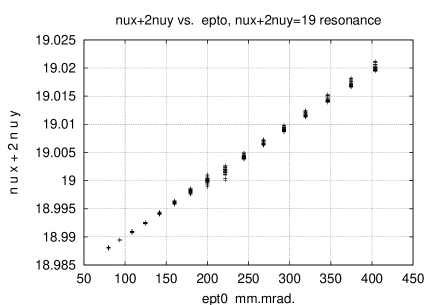
Figure 19: $\nu_{x}+2|nu_{y}$ vs $\epsilon_{t0}$ for the $\nu_{x}+2\nu_{y}=19$ resonance excited by a random $b_{2}$ in the SNS magnets and corrected using two sextupole correctors. The initial coordinates $x_{0},p_{x0},y_{0},p_{y0}$ lie along 6 directions in the $x_{0},p_{x0}$ phase space and 6 directions in $y_{0},p_{y0}$ space .$\nu_{x0}=6.3933$,$\nu_{y0}=6.2933$. In the figure x0,px0,y0,py0,epx0,ept0,nux0,nuy0 represent $x_{0},p_{x0},y_{0},p_{y0},\epsilon_{x0},\epsilon_{y0},\epsilon_{t0},\nu_{x0},\nu_{y0}$.

The correction of the island resonances for the $\nu_{x}+2\nu_{y}=19$ resonance can be done with two sextupole correctors properly located around the ring. Assuming that one has a way to measure either the width of the island or the maximun emittance growth using the above results as a guide , then the two correctors can be adjusted one at a time to reduce the emittance growth or the island width. Simulating this procedure gives the results shown in Fig. 18 and Fig. 19. The emittance growth ,the maximun $d\epsilon_{t,max}$, is reduced by almost a factor of 15 by the best setting of the correctors that was found. In this case, setting the correctors to zero the stopband, $d\nu_{12}$=0, reduces the maximun emittance growth by a factor of 5.

Higher order resonances

In the above, results were presented for the 3nux=19 and the $\nu_{x}+2\nu_{y}=19$ resonances. Similar studies have also been done for all four of the third order resonances $m\nu_{x}+n\nu_{y}=19$, $m+n=3$, and for all five of the fourth order resonances $m\nu_{x}+n\nu_{y}=25$, $m+n=4$, with similar results. It is our expectation that similar results would be found for the higher order resonance $m\nu_{x}+n\nu_{y}=q$, where m,n,q are integers. In particular, if $m\nu_{x}+n\nu_{y}$ is plotted versus $\epsilon_{t0}$, this plot will contain a flat region where $m\nu_{x}+n\nu_{y}$ is costant at $m\nu_{x}+n\nu_{y}=q$, and the width of this flat region will give the width of the islands associated with the $m\nu_{x}+n\nu_{y}=q$ resonance.

References

[1]Y. Papaphilippou and D.T. Abell, EPAC’00, p.1453. (2000)
[2]V. Ptitsyn, A.V. Fedotov, F. Pilat,EPAC’02, p.350,(2002)