TPC tracking and particle identification in high-density environment

Abstract

Track finding and fitting algorithm in the ALICE Time projection chamber (TPC) based on Kalman-filtering is presented. Implementation of particle identification (PID) using d$E$/d$x$ measurement is discussed. Filtering and PID algorithm is able to cope with non-Gaussian noise as well as with ambiguous measurements in a high-density environment. The occupancy can reach up to 40% and due to the overlaps, often the points along the track are lost and others are significantly displaced. In the present algorithm, first, clusters are found and the space points are reconstructed. The shape of a cluster provides information about overlap factor. Fast spline unfolding algorithm is applied for points with distorted shapes. Then, the expected space point error is estimated using information about the cluster shape and track parameters. Furthermore, available information about local track overlap is used. Tests are performed on simulation data sets to validate the analysis and to gain practical experience with the algorithm.

I Introduction

Track finding for the predicted particle densities is one of the most challenging tasks in the ALICE experiment ALICE . It is still under development and here the current status is reported. Track finding is based on the Kalman-filtering approach. Kalman-like algorithms are widely used in high-energy physics experiments and their advantages and shortcomings are well known.

There are two main disadvantages of the Kalman filter, which affect the tracking in the ALICE TPC TPCTDR . The first is that before applying the Kalman-filter procedure, clusters have to be reconstructed. Occupancies up to 40% in the inner sectors of the TPC and up to 20% in the outer sectors are expected; clusters from different tracks may be overlapped; therefore a certain number of the clusters are lost, and the others may be significantly displaced. These displacements are rather hard to take into account. Moreover, these displacements are strongly correlated depending on the distance between two tracks.

The other disadvantage of the Kalman-filter tracking is that it relies essentially on the determination of good ‘seeds’ to start a stable filtering procedure. Unfortunately, for the tracking in the ALICE TPC the seeds using the TPC data themselves have to be constructed. The TPC is a key starting point for the tracking in the entire ALICE set-up. Until now, practically none of the other detectors have been able to provide the initial information about tracks.

On the other hand, there is a whole list of very attractive properties of the Kalman-filter approach.

• It is a method for simultaneous track recognition and fitting.

• There is a possibility to reject incorrect space points ‘on the fly’, during the only tracking pass. Such incorrect points can appear as a consequence of the imperfection of the cluster finder. They may be due to noise or they may be points from other tracks accidentally captured in the list of points to be associated with the track under consideration. In the other tracking methods one usually needs an additional fitting pass to get rid of incorrectly assigned points.

• In the case of substantial multiple scattering, track measurements are correlated and therefore large matrices (of the size of the number of measured points) need to be inverted during a global fit. In the Kalman-filter procedure we only have to manipulate up to $5\times 5$ matrices (although many times, equal to the number of measured points), which is much faster.

• Using this approach one can handle multiple scattering and energy losses in a simpler way than in the case of global methods.

• Kalman filtering is a natural way to find the extrapolation of a track from one detector to another (for example from the TPC to the ITS or to the TRD).

The following parametrization for the track was chosen:

$$y(x)=y_{0}-\frac{\displaystyle 1}{\displaystyle C}\sqrt{1-({C}x-{\eta})^{2}}$$ (1)

$$z(x)=z_{0}-\frac{\displaystyle\tan\lambda}{\displaystyle C}\arcsin({C}x-{\eta})$$ (2)

The state vector $x^{\rm{T}}$ is given by the local track position x, y and z, by a curvature C, local x₀ position of the helix center, and dip angle $\lambda$:

$${\bf x}^{\rm{T}}=(y,\ z,\ C,\ \tan\lambda,\ \eta),~{}\eta\equiv Cx_{0}$$ (3)

Because of high occupancy the standard Kalman filter approach was modified. We tried to find maximum additional possible information which can be used during cluster finding, tracking and particle identification. Because of too many degrees of freedom (up to 220 million 10-bit samples) we have to find a smaller number of orthogonal parameters.

To enable using the optimal combination of local and global information about the tracks and clusters, the parallel Kalman filter tracking method was proposed. Several hypothesis are investigated in parallel. The global tracking approach such as Hough transform was considered only for seeding of track candidates. In the following, the additional information which was used will be underlined.

II Accuracy of local coordinate measurement

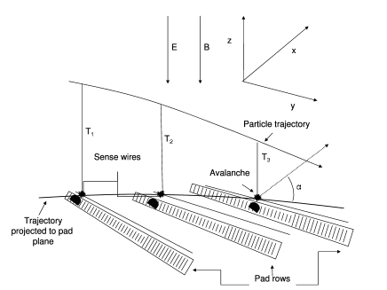
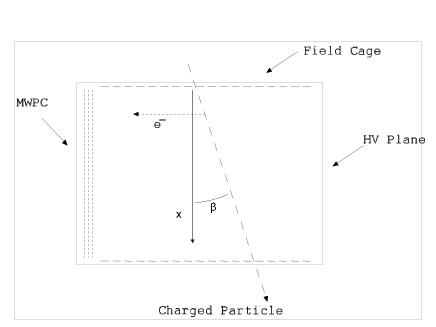
Figure 1: Schematic view of the detection process in TPC (upper part - perspective view, lower part - side view).

The accuracy of the coordinate measurement is limited by a track angle which spreads ionization and by diffusion which amplifies this spread.

The track direction with respect to pad plane is given by two angles $\alpha$ and $\beta$ (see fig. 1). For the measurement along the pad-row, the angle $\alpha$ between the track projected onto the pad plane and pad-row is relevant. For the measurement of the the drift coordinate (z–direction) it is the angle $\beta$ between the track and z axis (fig. 1).

The ionization electrons are randomly distributed along the particle trajectory. Fixing the reference x position of an electron at the middle of pad-row, the y (resp. z) position of the electron is a random variable characterized by uniform distribution with the width $L_{\rm{a}}$, where $L_{\rm{a}}$ is given by the pad length $L_{\rm{pad}}$ and the angle $\alpha$ (resp. $\beta$):

$$L_{\rm{a}}=L_{\rm{pad}}\tan\alpha$$

The diffusion smears out the position of the electron with gaussian probability distribution with $\sigma_{\rm{D}}$. Contribution of the $\mathbf{E{\times}B}$ and unisochronity effects for the Alice TPC are negligible. The typical resolution in the case of ALICE TPC is on the level of $\sigma_{y}\sim$ 0.8 mm and $\sigma_{z}\sim$ 1.0 mm integrating over all clusters in the TPC.

II.1 Gas gain fluctuation effect

Being collected on sense wire, electron is ”multiplied” in strong electric field. This multiplication is subject of a large fluctuations, contributing to the cluster position resolution. Because of these fluctuations the center of gravity of the electron cloud can be shifted.

Each electron is amplified independently. However, in the reconstruction electrons are not treated separately. The Centre Of Gravity (COG) of the cluster is usually used as an estimation for the local track position. The influence of the gas gain fluctuation to the reconstructed point characteristic can be described by a simple model, introducing a weighted COG $X_{\rm{COG}}$

$$X_{\rm{COG}}=\frac{\sum_{i=1}^{N}{g_{i}x_{i}}}{\sum_{i=1}^{N}{g_{i}}},$$ (4)

where N is the total number of electrons in the cluster and $g_{i}$ is a random variable equal to a gas amplification for given electron.

The mean value of $X_{\rm{COG}}$ is equal to the mean value $\overline{x}$ of the original distribution of electrons

$$\overline{X_{COG}}=\overline{\frac{\sum_{i=1}^{N}{g_{i}x_{i}}}{\sum_{i=1}^{N}{g_{i}}}}=\overline{x}\overline{\frac{\sum_{i=1}^{N}{g_{i}}}{\sum_{i=1}^{N}{g_{i}}}}=\overline{x}.$$ (5)

However, the same is not true for the dispersion of the position,

$$\sigma^{2}_{X_{\rm{COG}}}=\overline{X_{\rm{COG}}^{2}}-\overline{X_{\rm{COG}}}^{2}=$$ (6)

$${}=\overline{\left(\frac{1}{\sum_{i=1}^{N}{g_{i}}}\sum_{i=1}^{N}{g_{i}x_{i}}\right)^{2}}-\overline{x}^{2}=$$

$${}=\overline{\frac{{\sum\sum{x_{i}x_{j}g_{i}g_{j}}}}{{\sum\sum{g_{i}g_{j}}}}}-\overline{x}^{2}=$$

$${}=\overline{x^{2}}\overline{\frac{\sum_{i}{g_{i}^{2}}}{\sum\sum{g_{i}g_{j}}}}-\overline{x}^{2}\overline{\frac{\sum\sum{g_{i}g_{j}}-\sum\sum_{i\neq{j}}{g_{i}g_{j}}}{\sum\sum{g_{i}g_{j}}}}=$$

$$=\left(\overline{x^{2}}-\overline{x}^{2}\right)\overline{\frac{\sum{g_{i}^{2}}}{\sum\sum{g_{i}g_{j}}}}=\sigma_{x}^{2}\overline{\frac{\sum{g_{i}^{2}}}{\sum\sum{g_{i}g_{j}}}}=$$

$${}=\frac{\sigma_{x}^{2}}{N}{\times}G_{\rm{gfactor}}^{2}$$

where

$$G_{\rm{gfactor}}^{2}=N\overline{\frac{\sum{g_{i}^{2}}}{\sum\sum{g_{i}g_{j}}}}$$ (7)

The diffusion term is effectively multiplied by gas gain factor $G_{\rm{gfactor}}$. For sufficiently large number of electrons, when $g_{i}^{2}$ and $\sum\sum{g_{i}g_{j}}$ are quasi independent variables, equation (7) can be transformed to the following

$$G_{\rm{gfactor}}^{2}\approx N\frac{\overline{\sum{g_{i}^{2}}}}{\overline{\sum\sum{g_{i}g_{j}}}}$$ (8)

$${}=N\frac{N\overline{g^{2}}}{N(N-1)\overline{g}^{2}+N\overline{g^{2}}}=$$

$${}=N\frac{\left(\sigma_{g}^{2}/\overline{g}^{2}+1\right)}{N+\sigma_{g}^{2}/\overline{g}^{2}}$$

Gas gain fluctuation of the gas detector working in proportional regime is described with the exponential distribution with the mean value $\bar{g}$ and r.m.s.

$$\sigma_{\rm{g}}=\bar{g}$$ (9)

Substituting $\sigma_{\rm{g}}$ into equation (8)

$$G_{\rm{gfactor}}^{2}=\frac{2N}{N+1}.$$ (10)

Gas multiplication fluctuation in chamber deteriorates $\sigma_{X_{\rm{COG}}}$ by a factor of about ${\sqrt{2}}$. The prediction of this model is in good agreement with results from the simulation.

II.2 Secondary ionization effect

Charged particle penetrating the gas of the detector produces N primary electrons. Primary electron i produces $n_{\rm{s}}^{i}-1$ secondary electrons. Each of these electrons is amplified in the electric field by a factor of $g_{j}$.

Each primary cluster is characterized by a position $x_{i}$ with mean value $\overline{x}$ and $\sigma_{x}$. The COG given by equation (4) is modified to the following form:

$$X_{\rm{COG}}=\frac{1}{\sum_{i=1}^{N}\sum_{j=1}^{n_{i}}{g_{j}^{i}}}\sum_{i=1}^{N}{x_{i}}\sum_{j=1}^{n_{i}}{g_{j}^{i}}.$$ (11)

A new variable $G_{n}$ is introduced as the total electron gain:

$$G_{n}=\sum_{j=1}^{n}{g_{j}}.$$ (12)

Knowing the distribution of n and g and assuming that n and g are independent variables the mean value and variance of the $G_{n}$ can be expressed as:

$$\overline{G_{n}}=\overline{n}\overline{g}$$ (14)

$${}\frac{\sigma^{2}_{G_{n}}}{\overline{G_{n}^{2}}}=\frac{\sigma^{2}_{n}}{\overline{n}^{2}}+\frac{\sigma^{2}_{g}}{\overline{g}^{2}}\frac{1}{\overline{n}}$$

Inserting $G_{n}$ into equation (11) results in an equation similar to the equation (4).

Multiplicative factor $G_{\rm{Lfactor}}$ is defined as an analog of $G_{\rm{gfactor}}$, from the equation (7)

$$G_{\rm{Lfactor}}^{2}=N\frac{\overline{\sum{G_{i}^{2}}}}{\overline{\sum\sum{G_{i}G_{j}}}}.$$ (15)

Using the new variable $G_{n}$ and simply replacing gas gain g by $G_{n}$ in the similar way as in equation (8) does not work. For $1/E^{2}$ parametrization of secondary ionization process $\sigma^{2}_{G_{n}}/\overline{G_{n}}$ goes to infinity and thus $\sigma^{2}_{X_{COG}}=\sigma_{x}^{2}$. Moreover $G_{i}^{2}$ and $\sum\sum{G_{i}G_{j}}$ are not quasi independent as the sum $\sum\sum{G_{i}G_{j}}$ could be given by one ”exotic” electron cluster. Approximations used for deriving the equation (8) are not valid for secondary ionization effect.

In order to estimate the impact of this effect on COG equation (15) has to be solved numerically. Simulation showed that $G_{\rm{Lfactor}}$ does not depend strongly on the cut used for maximum number of electrons created in the process of secondary ionization. A change of the cut, from 1000 electrons up produces a change of about 3% in $G_{\rm{Lfactor}}$.

Equation (8) is not applicable in this situation because of the infinity of the $\sigma_{G}$. According to the simulation, the threshold on the number of electrons in the cluster has a little influence to the resulting $G_{\rm{Lfactor}}$. Therefore we fit simulated $G_{\rm{Lfactor}}$ with formula (8) where $\sigma_{G}^{2}/\overline{G}^{2}$ was a free parameter. However, this parametrization does not describe the data for wide enough range of N. In further study the linear parametrization of the COG factor was used. This parametrization was validated on reasonable interval of N.

III Center-of-gravity error parametrization

Detected position of charged particle is a random variable given by several stochastic processes: diffusion, angular effect, gas gain fluctuation, Landau fluctuation of the secondary ionization, $\mathbf{E{\times}B}$ effect, electronic noise and systematic effects (like space charge, etc.). The relative influence of these processes to the resulting distortion of position determination depends on the detector parameters. In the big drift detectors like the ALICE TPC the main contribution is given by diffusion, gas gain fluctuation, angular effect and secondary ionization fluctuation.

Furthermore we will use following assumptions:

• $N_{\rm{prim}}$ primary electrons are produced at a random positions $x_{i}$ along the particle trajectory.

• $n_{i}-1$ electrons are produced in the process of secondary ionization.

• Displacement of produced electrons due to the thermalization is neglected.

Each of electrons is characterized by a random vector $\vec{z}^{i}_{j}$

$$\vec{z}^{i}_{j}=\vec{x}^{i}+\vec{y}^{i}_{j},$$ (16)

where i is the index of primary electron cluster and j is the index of the secondary electron inside of the primary electron cluster. Random variable $\vec{x}^{i}$ is a position where the primary electron was created. The position $\vec{y}^{i}_{j}$ is a random variable specific for each electron. It is given mainly by a diffusion.

The center of gravity of the electron cloud is given:

$$\vec{z}_{\rm{COG}}=\frac{1}{\sum_{i=1}^{N_{\rm{prim}}}\sum_{j=1}^{n_{i}}{g_{j}^{i}}}\sum_{i=1}^{N_{\rm{prim}}}\sum_{j=1}^{n_{i}}{g_{j}^{i}\vec{z}_{j}^{i}}=$$ (17)

$${}\frac{1}{\sum_{i=1}^{N_{\rm{prim}}}\sum_{j=1}^{n_{i}}{g_{j}^{i}}}\sum_{i=1}^{N_{\rm{prim}}}\vec{x}^{i}\sum_{j=1}^{n_{i}}{g_{j}^{i}}+$$

$${}\frac{1}{\sum_{i=1}^{N_{\rm{prim}}}\sum_{j=1}^{n_{i}}{g_{j}^{i}}}\sum_{i=1}^{N_{\rm{prim}}}\sum_{j=1}^{n_{i}}{g_{j}^{i}\vec{y}_{j}^{i}}=$$

$${}\vec{x}_{\rm{COG}}+\vec{y}_{\rm{COG}}.$$

The mean value $\overline{\vec{z}_{\rm{COG}}}$ is equal to the sum of mean values $\overline{\vec{x}_{\rm{COG}}}$ and $\overline{\vec{y}_{\rm{COG}}}$.

The sigma of COG in one of the dimension of vector $\vec{z}_{1COG}$ is given by following equation

$$\sigma_{z_{\rm{1COG}}}^{2}=\sigma_{x_{\rm{1COG}}}^{2}+\sigma_{y_{\rm{1COG}}}^{2}+$$ (18)

$${}2\left(\overline{x_{\rm{1COG}}y_{\rm{1COG}}}-\bar{x}_{\rm{1COG}}\bar{y}_{1COG}\right).$$

If the vectors $\vec{x}$ and $\vec{y}$ are independent random variables the last term in the equation (18) is equal to zero.

$$\sigma_{z_{1COG}}^{2}=\sigma_{x_{\rm{1COG}}}^{2}+\sigma_{y_{\rm{1COG}}}^{2},$$ (19)

r.m.s. of COG distribution is given by the sum of r.m.s of x and y components.

In order to estimate the influence of the $\mathbf{E{\times}B}$ and unisochronity effect to the space resolution two additional random vectors are added to the initial electron position.

$$\vec{z}^{i}_{j}=\vec{x}^{i}+\vec{y}^{i}_{j}+\vec{X}_{\mathbf{E{\times}B}}(\vec{x}^{i}+\vec{y}^{i}_{j})+\vec{X}_{\rm{Unisochron}}(\vec{x}^{i}+\vec{y}^{i}_{j}).$$ (20)

The probability distributions of $\vec{X}_{\mathbf{E{\times}B}}$ and $\vec{X}_{\rm{Unisochron}}$ are functions of random vectors $\vec{x^{i}}$ and $\vec{y^{i}_{j}}$, and they are strongly correlated. However, simulation indicates that in large drift detectors distortions, due to these effects, are negligible compared with a previous one.

Combining previous equation and neglecting $\mathbf{E{\times}B}$ and unisochronity effects, the COG distortion parametrization appears as:
$\sigma_{z}$ of cluster center in z (time) direction

$$\sigma^{2}_{{z_{\rm{COG}}}}=\frac{D^{2}_{\rm{L}}L_{\rm{Drift}}}{N_{\rm{ch}}}G_{\rm{g}}+$$ (21)

$${}\frac{{\tan^{2}\alpha}~{}L_{\rm{pad}}^{2}G_{\rm{Lfactor}}(N_{\rm{chprim}})}{12N_{\rm{chprim}}}+\sigma^{2}_{\rm{noise}},$$

and $\sigma_{y}$ of cluster center in y(pad) direction

$$\sigma^{2}_{y_{\rm{COG}}}=\frac{D^{2}_{\rm{T}}L_{\rm{Drift}}}{N_{\rm{ch}}}G_{\rm{g}}+$$ (22)

$${}\frac{{\tan^{2}\beta}~{}L_{\rm{pad}}^{2}G_{\rm{Lfactor}}(N_{\rm{chprim}})}{12N_{\rm{chprim}}}+\sigma^{2}_{\rm{noise}},$$

where ${N_{\rm{ch}}}$ is the total number of electrons in the cluster, ${N_{\rm{chprim}}}$ is the number of primary electrons in the cluster, ${G_{\rm{g}}}$ is the gas gain fluctuation factor, ${G_{\rm{Lfactor}}}$ is the secondary ionization fluctuation factor and $\sigma_{\rm{noise}}$ describe the contribution of the electronic noise to the resulting sigma of the COG.

IV Precision of cluster COG determination using measured amplitude

We have derived parametrization using as parameters the total number of electrons ${N_{\rm{ch}}}$ and the number of primary electrons ${N_{\rm{chprim}}}$. This parametrization is in good agreement with simulated data, where the ${N_{\rm{ch}}}$ and ${N_{\rm{chprim}}}$ are known. It can be used as an estimate for the limits of accuracy, if the mean values $\overline{N}_{\rm{ch}}$ and $\overline{N}_{\rm{chprim}}$ are used instead.

The ${N_{\rm{ch}}}$ and ${N_{\rm{chprim}}}$ are random variables described by a Landau distribution, and Poisson distribution respectively .

In order to use previously derived formulas (21, 22), the number of electrons can be estimated assuming their proportionality to the total measured charge $A$ in the cluster. However, it turns out that an empirical parametrization of the factors $G(N)/N=G(A)/(kA)$ gives better results. Formulas (21) and (22) are transformed to following form:

$\sigma_{z}$ of cluster center in z (time) direction:

$$\sigma^{2}_{z_{\rm{COG}}}=\frac{D^{2}_{\rm{L}}L_{\rm{Drift}}}{A}{\times}\frac{G_{g}(A)}{k_{\rm{ch}}}+$$ (23)

$${}\frac{\tan^{2}\alpha~{}L_{\rm{pad}}^{2}}{12A}{\times}\frac{G_{Lfactor}(A)}{k_{\rm{prim}}}+\sigma^{2}_{\rm{noise}}$$

and $\sigma_{y}$ of cluster center in y(pad) direction:

$$\sigma_{y_{\rm{COG}}}=\frac{D^{2}_{\rm{T}}L_{\rm{Drift}}}{A}{\times}\frac{G_{g}(A)}{k_{\rm{ch}}}+$$ (24)

$${}\frac{\tan^{2}\beta~{}L_{\rm{pad}}^{2}}{12A}{\times}\frac{G_{Lfactor}(A)}{k_{\rm{prim}}}+\sigma^{2}_{\rm{noise}}$$

V Estimation of the precision of cluster position determination using measured cluster shape

The shape of the cluster is given by the convolution of the responses to the electron avalanches. The time response function and the pad response function are almost gaussian, as well as the spread of electrons due to the diffusion. The spread due to the angular effect is uniform. Assuming that the contribution of the angular spread does not dominate the cluster width, the cluster shape is not far from gaussian. Therefore, we can use the parametrization

$$f(t,p)=K_{\rm{Max}}.\exp\left(-\frac{(t-t_{\rm{0}})^{2}}{2\sigma_{\rm{t}}^{2}}-\frac{(p-p_{\rm{0}})^{2}}{2\sigma_{\rm{p}}^{2}}\right),$$ (25)

where ${K_{\rm{Max}}}$ is the normalization factor, $t$ and $p$ are time and pad bins, $t_{0}$ and $p_{0}$ are centers of the cluster in time and pad direction and $\sigma_{\rm{t}}$ and $\sigma_{\rm{p}}$ are the r.m.s. of the time and pad cluster distribution.

The mean width of the cluster distribution is given by:

$$\sigma_{\rm{t}}=\sqrt{D{\rm{{}^{2}_{L}}}L_{\rm{drift}}+\sigma^{2}_{\rm{preamp}}+\frac{\tan^{2}\alpha~{}L_{\rm{pad}}^{2}}{12}},$$ (26)

$$\sigma_{\rm{p}}=\sqrt{D{\rm{{}^{2}_{T}}}L_{\rm{drift}}+\sigma^{2}_{\rm{PRF}}+\frac{\tan^{2}\beta~{}L_{\rm{pad}}^{2}}{12}},$$ (27)

where ${\sigma_{\rm{preamp}}}$ and ${\sigma_{\rm{PRF}}}$ are the r.m.s. of the time response function and pad response function, respectively.

The fluctuation of the shape depends on the contribution of the random diffusion and angular spread, and on the contribution given by a gas gain fluctuation and secondary ionization. The fluctuation of the time and pad response functions is small compared with the previous one.

The measured r.m.s of the cluster is influenced by a threshold effect.

$$\sigma_{\rm{t}}^{2}=\sum_{A(t,p)>\rm{threshold}}{(t-t_{\rm{0}})^{2}{\times}A(t,p)}$$ (28)

The threshold effect can be eliminated using two dimensional gaussian fit instead of the simple COG method. However, this approach is slow and, moreover, the result is very sensitive to the gain fluctuation.

To eliminate the threshold effect in r.m.s. method, the bins bellow threshold are replaced with a virtual charge using gaussian interpolation of the cluster shape. The introduction of the virtual charge improves the precision of the COG measurement. Large systematic shifts in the estimate of the cluster position (depending on the local track position relative to pad–time) due to the threshold are no longer observed.

Measuring the r.m.s. of the cluster, the local diffusion and angular spread of the electron cloud can be estimated. This provides additional information for the estimation of distortions. A simple additional correction function is used:

$$\sigma_{\rm{COG}}\rightarrow\sigma_{\rm{COG}}(A){\times}(1+{\rm{const}{\times}\frac{\delta\rm{RMS}}{\rm{teorRMS}}}),$$ (29)

where $\sigma_{\rm{COG}}(A)$ is calculated according formulas 22 and 21, and the $\delta\rm{RMS}/\rm{teorRMS}$ is the relative distortion of the signal shape from the expected one.

VI TPC cluster finder

The classical approach for the beginning of the tracking was chosen. Before the tracking itself, two-dimensional clusters in pad-row–time planes are found. Then the positions of the corresponding space points are reconstructed, which are interpreted as the crossing points of the tracks and the centers of the pad rows. We investigate the region 5$\times$5 bins in pad-row–time plane around the central bin with maximum amplitude. The size of region, 5$\times$5 bins, is bigger than typical size of cluster as the $\sigma_{\rm{t}}$ and $\sigma_{\rm{pad}}$ are about 0.75 bins.

The COG and r.m.s are used to characterize cluster. The COG and r.m.s are affected by systematic distortions induced by the threshold effect. Depending on the number of time bins and pads in clusters the COG and r.m.s. are affected in different ways. Unfortunately, the number of bins in cluster is the function of local track position. To get rid of this effect, two-dimensional gaussian fitting can be used.

Similar results can be achieved by so called r.m.s. fitting using virtual charge. The signal below threshold is replaced by the virtual charge, its expected value according a interpolation. If the virtual charge is above the threshold value, then it is replaced with amplitude equal to the threshold value. The signal r.m.s is used for later error estimation and as a criteria for cluster unfolding. This method gives comparable results as gaussian fit of the cluster but is much faster. Moreover, the COG position is less sensitive to the gain fluctuations.

The cluster shape depends on the track parameters. The response function contribution and diffusion contribution to the cluster r.m.s. are known during clustering. This is not true for a angular contribution to the cluster width. The cluster finder should be optimised for high momentum particle coming from the primary vertex. Therefore, a conservative approach was chosen, assuming angle $\alpha$ to be zero. The tangent of the angle $\beta$ is given by z-position and pad-row radius, which is known during clustering.

VI.1 Cluster unfolding

The estimated width of the cluster is used as criteria for cluster unfolding. If the r.m.s. in one of the directions is greater then critical r.m.s, cluster is considered for unfolding. The fast spline method is used here. We require the charge to be conserved in this method. Overlapped clusters are supposed to have the same r.m.s., which is equivalent to the same track angles. If this assumption is not fulfilled, tracks diverge very rapidly.

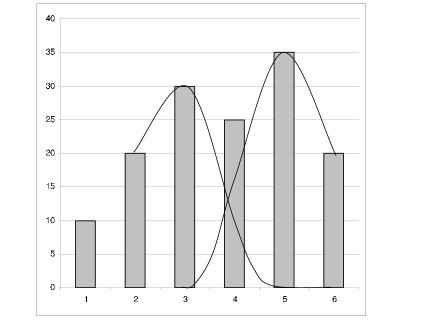
Figure 2: Schematic view of unfolding principle.

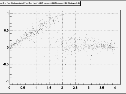
Figure 3: Dependence of the position residual as function of the distance to the second cluster.

The unfolding algorithm has the following steps:

• Six amplitudes $C_{i}$ are investigated (see fig. 2). First (left) local maxima, corresponding to the first cluster is placed at position 3, second (right) local maxima corresponding to the second cluster is at position 5.

• In the first iteration, amplitude in bin 4 corresponding to the cluster on left side $A_{\rm{L4}}$ is calculated using polynomial interpolation, assuming virtual amplitude at $A_{\rm{L5}}$ and derivation at $A_{\rm{L5}}^{{}^{\prime}}$ to be 0. Amplitudes $A_{\rm{L2}}$ and $A_{\rm{L3}}$ are considered to be not influenced by overlap ($A_{\rm{L2}}=C_{2}$ and $A_{\rm{L3}}=C_{3})$.

• The amplitude $A_{\rm{R4}}$ is calculated in similar way. In the next iteration the amplitude $A_{\rm{L4}}$ is calculated requiring charge conservation $C_{\rm{4}}=A_{\rm{R4}}+A_{\rm{L4}}$. Consequently

  $$A_{\rm{L4}}\rightarrow C_{\rm{4}}\frac{A_{\rm{L4}}}{A_{\rm{L4}}+A_{\rm{R4}}}$$ (30)

  and

  $$A_{\rm{R4}}\rightarrow C_{\rm{4}}\frac{A_{\rm{R4}}}{A_{\rm{L4}}+A_{\rm{R4}}}.$$ (31)

Two cluster resolution depends on the distance between the two tracks. Until the shape of cluster triggers unfolding, there is a systematic shifts towards to the COG of two tracks (see fig. 3), only one cluster is reconstructed. Afterwards, no systematic shift is observed.

VI.2 Cluster characteristics

The cluster is characterized by the COG in y and z directions (fY and fZ) and by the cluster width (fSigmaY, fSigmaZ). The deposited charge is described by the signal at maximum (fMax), and total charge in cluster (fQ). The cluster type is characterized by the data member fCType which is defined as a ratio of the charge supposed to be deposited by the track and total charge in cluster in investigated region 5$\times$5. The error of the cluster position is assigned to the cluster only during tracking according formulas (23) and (24), when track angles $\alpha$ and $\beta$ are known with sufficient precision.

Obviously, measuring the position of each electron separately the effect of the gas gain fluctuation can be removed, however this is not easy to implement in the large TPC detectors. Additional information about cluster asymmetry can be used, but the resulting improvement of around 5% in precision on simulated data is negligible, and it is questionable, how successful will be such correction for the cluster asymmetry on real data.

However, a cluster asymmetry can be used as additional criteria for cluster unfolding. Let’s denote $\mu_{i}$ the i-th central momentum of the cluster, which was created by overlapping from two sub-clusters with unknown positions and deposited energy (with momenta ${}^{1}\mu_{i}$ and ${}^{2}\mu_{i}$).

Let $r_{1}$ is the ratio of two clusters amplitudes:

$$r_{1}={{}^{1}\mu_{0}}/({{}^{1}\mu_{0}}+{{}^{2}\mu_{0}})$$

and the track distance d is equal to

$$d={{}^{1}\mu_{1}}-{{}^{2}\mu_{1}}.$$

Assuming that the second moments for both sub-clusters are the same (${{}^{0}\mu_{2}}={{}^{1}\mu_{2}}={{}^{2}\mu_{2}}$), two sub-clusters distance d and amplitude ratio $r_{1}$ can be estimated:

$$R=\frac{(\mu_{3}^{6})}{(\mu_{2}^{2}-{{}^{0}\mu_{2}^{2}})^{3}}$$ (32)

$$r_{\rm{1}}=0.5\pm 0.5{\times}\sqrt{\frac{1}{1-4/R}}$$ (33)

$$d=\sqrt{(4+R){\times}(\mu_{2}^{2}-{{}^{0}\mu_{2}^{2}})}$$ (34)

In order to trigger unfolding using the shape information additional information about track and mean cluster shape over several pad-rows are needed. This information is available only during tracking procedure.

VI.3 TPC seed finding

The first and the most time-consuming step in tracking is seed finding. Two different seeding strategies are used, combinatorial seeding with vertex constraint and simple track follower.

VI.4 Combinatorial seeding algorithm

Combinatorial seeding starts with a search for all pairs of points in the pad-row number i1 and in a pad-row i2, $n$ rows closer to the interaction point ($n=i1-i2=20$ at present) which can project to the primary vertex. The position of the primary vertex is reconstructed, with high precision, from hits in the ITS pixel layers, independently of the track determination in the TPC.

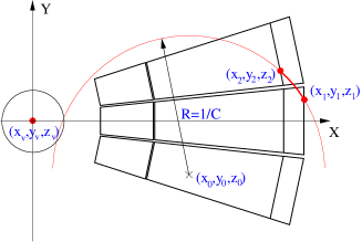
Figure 4: Schematic view of the combinatorial seeding procedure

Algorithm of combinatorial seeding consists of following steps;

• Loop over all clusters on pad-row i1

  • Loop over all clusters on pad-row i2, inside a given window. The size of the window is defined by a cut on track curvature (C), requiring to seed primary tracks with $p_{\rm{t}}$ above a threshold.

    • When a reasonable pair of clusters is found, parameters of a helix going through these points and the primary vertex are calculated. Parameters of this helix are taken as an initial approximation of the parameters of the potential track. The corresponding covariance matrix is evaluated using the point errors, which are given by the cluster finder, and applying an uncertainty of the primary vertex position. This is the only place where a certain (not too strong) vertex constraint was introduced. Later on, tracks are allowed to have any impact parameters at primary vertex in both the $z$-direction and in $r$-$\varphi$ plane.

    • Using the calculated helix parameters and their covariance matrix the Kalman filter is started from the outer point of the pair to the inner one.

    • If at least half of the potential points between the initial ones were successfully associated with the track candidate, the track is saved as a seed.

  • End of loop over pad-row 2

• End of loop over pad-row 1

VI.5 Track following seeding algorithm

Seeding between two pad-rows, i1 and i2, starts in the middle pad-row. For each cluster in the middle pad-row, the two nearest clusters in the pad-row up and down are found. Afterwards, a linear fit in both directions (z and y) is calculated. Expected prolongation to the next two pad-rows are calculated. For next prolongation again two nearest clusters are found. Algorithm continue recursively up to the pad-rows i1 and i2. The linear fit is replaced by polynomial after 7 clusters. If more than half of the potential clusters are found, the track parameters and covariance are calculated as before.

VI.6 Seed finding strategy

Table 1: Combinatorial seeding efficiency and time consumption as a function of the distance between two pad-rows.

distance	time	efficiency[%]
24	95s	92.2
20	52s	90.4
16	34s	88.7
14	25s	88.1
12	19s	85.2

The main advantage of combinatorial seeding is high efficiency, around 90% for primaries with $p_{\rm{t}}>200\rm{MeV/c}$. The main disadvantage is the $N^{2}$ problem of the combinatorial search. The $N^{2}$ problem can be reduced restricting the size of the seeding window. This should be achieved by making the distance between seeding pad-rows smaller as the size of the window is proportional to $i2-i1$. However, decreasing the seeding distance, efficiency of seeding and also quality of seeds deteriorates. The size of the window can be reduced also by reducing the threshold curvature of the track candidate.

However, vertex constraint suppresses secondaries, which should be found also. The track following seeding has to be used for them. This strategy is much faster but less efficient (80%). The efficiency is decreased mainly due to effect of track overlaps and for low-$p_{\rm{t}}$ tracks by angular effect, which correlates the cluster position distortion between neighborhood pad-rows.

The efficiency of seeding can be increased repeating of the seeding procedure in different layers of the TPC. Assuming that overlapped tracks are random background for the track which should be seeded, the total efficiency of the seeding can be expressed as

$$\epsilon_{\rm{all}}=1-\prod{(1-\epsilon_{i})},$$

where $\epsilon_{i}$ is a efficiency of one seeding. Repeating seeding, efficiency should reach up to 100%. Unfortunately, tracks are sometimes very close on the long path and seeding in different layers can not be considered as independent. The efficiency of seeding saturate at a smaller value then 1. Another problem with repetitive seeding is that occupancy increases towards to the lower pad-row radius and thus the efficiency is a function of a the pad-row radius.

However, in order to find secondaries from kinks or V0 decay, it is necessary to make a high efficient seeding in outermost pad-rows. On the other hand in the case of kinks, in the high density environment it is almost impossible to start tracking of the primary particles using only the last point of the secondary track because this point is not well defined. In order to find them, seeding in innermost pad-rows should be performed. In both seeding strategies, large decrease of efficiency and precision due to the dead zones is observed. Additional seeding at the sector edges is necessary. The length of the pads for the outermost 30 pad-rows is greater than for the other pad-rows. The minimum of the occupancy and the maximum of seeding efficiency is obtained when we use outer pad-rows. In order to maximize tracking efficiency for secondaries it is necessary to make almost continual seeding inside of the TPC. Several combination of the slow combinatorial and the fast seeding were investigated. Depending on the required efficiency, different amount of the time for seeding can be spent. The default seeding for tracking performance results was chosen as following: two combinatorial seedings at outermost 20 pad-rows, and six track following seedings homogenously spaced inside the outermost sector.

More sophisticated and faster seeding is currently under development. It is planned to use, for seeding, only the clusters which were not assigned to tracks classified as almost perfect. The criteria for the almost perfect track has to be defined, depending on track density.

VII Parallel Kalman tracking

After seeding, several track hypothesis are tracked in parallel. Following algorithm is used:

• For each track candidate the prolongation to the next pad-row is found.

• Find nearest cluster.

• Estimate the cluster position distortions according track and cluster parameters.

• Update track according current cluster parameters and errors.

• Remove overlapped track hypotheses, i.e. those which share too many clusters together.

• Stop not active hypotheses.

• Continue down to the last pad-row.

The prolongation to the next pad-row is calculated according current track hypothesis. Distortions of the local track position $\sigma_{y}$ and $\sigma_{x}$ are calculated according covariance matrix. For each track prolongation a window is calculated. The width of the window is set to $\pm$4$\sigma$ where $\sigma$ is given by the convolution of the predicted track error and predicted expectation for cluster r.m.s. Clusters in the container are ordered according coordinates, binomial search with log(n) performance is used. The nearest cluster is taken maximal probable. No cluster competition is currently implemented because of the memory required when branching the Kalman track hypothesis and because of the performance penalty.

The width of the search window was chosen to take into account also overlapped clusters. The position error in this case could be significantly larger than estimated error for not overlapped cluster, and the overlap factor is not known apriori. On the other hand, the minimal distance between two reconstructed clusters is restricted by a local maxima requirement. Two clusters with distance less the $\sim$2 bins ($\sim$1 cm) can not be observed.

Once, the nearest cluster is found the cluster error is estimated using the cluster position and the amplitude according formulas (24) and (23). The correction for the cluster shape and overlapped factor is calculated according formula (29).

The cluster is finally accepted if the square of residuals in both direction is smaller than estimated 3$\sigma$. If this is the case track parameters are updated according cluster position and the error estimates.

It may occur that the track leaves the TPC sector and enters another one. In this case the track parameters and the covariance matrix is recalculated so that they are always expressed in the local coordinate system of the sector within which the track is at that moment. The variable fNFindable is defined as a number of potentially findable clusters. If track is locally inside the sensitive volume, the fNFindable is incremented otherwise remains unchanged.

If there are no clusters found in several pad-rows in active region of the TPC, track hypothesis should be removed. The cluster density is defined to measure the density of accepted clusters to all findable clusters in the region, where region is several pad-rows.

It is not known apriori, if a given track is primary or secondary, therefore local density can not be interpreted definitely as real density. This would be true only for tracks which really go through all considered pad-rows. Tracks with low local density are not completely removed, they are only signed (fRemoval variable) for the next analysis.

In order to be able to remove track hypotheses which are almost the same so called overlap factor is defined. It is the ratio of the clusters shared between two tracks candidates and the number of all clusters. If the overlap factor is greater than the threshold, track candidate with higher $\chi$2 or significantly lower number of points is removed. The threshold is parameter, currently we use the value (in performance studies) at 0.6. This is a compromise between the maximal efficiency requirement and minimal number of double found tracks requirement. In the future this parameters will be optimized, to increase double track resolution. In this case a new criteria to remove double found tracks will have to be used.

VII.1 Double track resolution

In the ALICE TPC represents the main challenge for tracking the large track density. From some distance between two tracks the clusters are not resolved anymore. In our algorithm the track candidates are removed if some fraction of the clusters are common to two track candidates. There are three possibilities, if the two tracks are overlapped on a very long path. Either it is the same track, or the two very close tracks or the two tracks where one changed direction to the second one, and the change of the direction was misinterpreted as multiple scattering.

New criteria should be defined to handle this situation. Cluster shape can be used again for this purpose. If the two tracks overlap and their separation is too small, only one cluster is reconstructed, however, its width is systematically greater. Moreover, the charge deposited in the cluster is also systematically higher.

Another problem is with double found clusters mainly at the low-$p_{\rm{t}}$ region. There are two reasons:

• The non gaussian tail of Coulomb scattering could change the direction of the track, track can be lost and found again during the next seeding.

• Because of large inclination and Landau fluctuations clusters with double local maxima could be created.

In order to maximize double-track resolution, and to minimize the number of double found tracks, the new criteria (mean local deposited charge and mean local cluster shape) are under investigation.

VII.2 d$E$/d$x$ measurement

To estimate particle mean ionization energy loss d$E$/d$x$, logarithmic truncated mean is used. Using the current cluster finder the truncation at 60% gives the best d$E$/d$x$ resolution. Currently the amplitudes at local cluster maxima are used, instead of the total cluster charge, in order to avoid the distortion due to the track overlaps. Shared clusters are not used for the estimate of the d$E$/d$x$ at all.

The measured amplitude is normalized to the track length, given by angles $\alpha$ and $\beta$ and by the pad length. Specific normalization factors are used for each pad type as the electronic parameters (gas gain, pad response function) are different in different parts of the TPC. The normalization condition requires the same d$E$/d$x$ inside each part of the TPC for one track.

Correlation between the measured d$E$/d$x$ and particle multiplicity was observed. The additional correction function for the cluster shape was successfully introduced, to take into account local clusters overlaps.

	no
$\sigma_{\phi}$[mrad]	1.399$\pm$0.030
$\sigma_{\Theta}$[mrad]	0.997$\pm$0.018
$\sigma_{p_{\rm{t}}}$[%]	0.881$\pm$0.011
$\sigma_{dEdx}/dEdx$[%]	6.00$\pm$0.2
$\epsilon$ [%]	99.0

Table 2: TPC tracking performance (dN/dy=4000 charged primaries)

VIII Conclusions

We have described current development in the ALICE TPC tracking which is one of the most challenging task in this experiment. The track finding efficiency increases, compared to the previous attempts, for primary tracks by about 10%, and even more for secondary tracks. The main improvement is a consequence of the sophisticated cluster finding and deconvolution which is based on detail understanding of the physical processes in the TPC and the optimal usage of achievable information. Another factor which helped in efficiency increase, especially for secondary tracks, is the new seeding procedure. The ALICE TPC tracker fulfil, and even exceeds the basic requirement. Further development will be concentrated on secondary vertexing inside TPC and possible use of information from other detectors.

References

- (1) ALICE Collaboration, Tecnical proposal, CER/LHCC/95-71
- (2) ALICE Collaboration, ALICE Technical Design Report of the Time Projection Chamber