Deterministic instabilities in the magneto-optical trap

Abstract

The cloud of cold atoms obtained from a magneto-optical trap is known to exhibit two types of instabilities in the regime of high atomic densities: stochastic instabilities and deterministic instabilities. In the present paper, the experimentally observed deterministic dynamics is described extensively. Three different behaviors are distinguished. All are cyclic, but not necessarily periodic. Indeed, some instabilities exhibit a cyclic behavior with an erratic return time. A one-dimensional stochastic model taking into account the shadow effect is shown to be able to reproduce the experimental behavior, linking the instabilities to a several bifurcations. Erraticity of some of the regimes is shown to be induced by noise.

1 Introduction

Experimental quantum physics knows since several years spectacular results, thanks to a simplification to produce quantum objects with long coherence times or macroscopic dimensions. Let us cite the achievement of the Bose-Einstein condensatesnobel , the characterization of quantum chaos QC , the improvement of atomic clocksclocks , the designs of quantum computers and quantum communication systemsqcomp , or also the accurate understanding of quantum decoherencedeco . One of the basic tools used to obtain most of these results is the Magneto-Optical Trap (MOT), which performs the cooling of atoms at temperatures of the order of the $\mu$K: this is the first step before reaching lower temperatures where the quantum properties of atoms dominate. Although it is a key device in the new atomic physics, the basic mechanisms determining the properties of the cloud of cold atoms in a MOT have been poorly studied, and the collective dynamics of these still “classical” atoms have been almost ignored, even though the existence of instabilities in the MOT is known since the first realizations. On the contrary, some simple empirical rules are used to avoid these inconveniences. Nevertheless, an accurate knowledge of the individual and collective behaviors of the cold atoms in the cloud could help in understanding the limitations of the process, and above all, to enhance it through the control of the dynamics, as it was done in many other systems, in physics and other fields of science.

However, a necessary preamble to such applications is the identification of the nature of the dynamics observed in MOTs. Indeed, complex behaviors may be subdivided in two groups: stochastic and deterministic behaviors. For the former, the dynamics originate in noise, i.e. in dynamical components, usually with a large number of degrees of freedom, considered as external to the system. This is usually experimental technical noise, and requires to add in the model a random component. Such a complex dynamics is meaningless from the physical point of view, because it cannot give any new informations about the MOT mechanisms. On the contrary, deterministic dynamics are intrinsic to the system, and do not require to add anything to the model: periodic instabilities can appear with two degrees of freedom, while chaos needs at least three degrees of freedom. This last case opens many perspectives: for example, it is possible to reach new working points by the methods of control of chaos, or to measure parameters which are usually inaccessiblebistab .

Recent studies have shown that the collective behavior of the atomic cloud produced by a MOT exhibit both stochastic instabilitiesnousprl ; bruit2002 and deterministic instabilitiesInstDet . The former has been extensively described in bruit2002 . A model demonstrates that the different stochastic behaviors observed in the experiments are well explained if the absorption of light by the atoms is taken into account, through the so-called shadow effect shadow . It is also shown that these stochastic instabilities are not “instabilities” in the usual meaning, as they result from an amplification of noise, due, from a dynamical point of view, to the folded structure of the stationary solutions. The same model was also predicting, for slighly different values of the parameters, deterministic instabilities which, in turn, has been observed experimentallyInstDet .

In the present paper, we report an extensive study of these deterministic instabilities. We detail and complete the experimental results given in InstDet , and analyze accurately the mechanisms leading to the different deterministic regimes through the model introduced in InstDet . We show in particular that the model is able to reproduce each type of dynamics, and predicts deterministic chaos. We show also the main role that noise is still playing in the dynamics.

The paper is organized as follows. After this introduction, section 2 describes briefly the experimental setup, and section 3 gives a detailed analysis of the experimental observations. Section 4 is devoted to a short description of the model, already detailed in bruit2002 . In section 5, the stationary solutions of the model are discussed, and in section 6, the deterministic dynamical behavior predicted by the model is described, and compared with the experiment results. Finally, in section 7, the effect of noise on the dynamics is studied.

2 Experimental set-up

The experimental set-up has already been described in detail elsewherebruit2002 , and thus the description here is simplified. The Cesium-atom MOT is in the usual $\sigma_{+}-\sigma_{-}$ configuration, with three arms of two counter-propagating beams obtained from the same laser diode. The waist $w_{T}$ of the trap beams may be varied from typically $3$ to $10$ mm. We use a configuration where counter-propagating beams result from the reflection of the three forward beams. This simplifies the detection of the dynamics, as compared to a six independent beams configuration. Indeed, because of the shadow effect, a center-of-mass motion is generated. However, as the nonlinearities involved in both cases are the same, we expect that the dynamics will be fundamentally of the same nature in the two configurations.

The dynamics of the atomic cloud consists in a deformation of the spatial atomic distribution, leading to fluctuations of the shape of the cloud, as illustrated in Fig. 1. Therefore, the relevant dynamical variables allowing us to describe instabilities, could be the shape of the cloud (i.e. for example the local velocities and atomic densities in the cloud). This type of description corresponds to a high dimensional model, associated with partial differential equations. Here, for the sake of simplicity, we choose to limit our description to the center of mass (CM) location ${\bf r}$, and the total number of atoms $n$ in the atomic cloud. This allows us to model the system with ordinary differential equations, and reduces the dimension to seven, and even three in a 1D model. As it is shown in the following, the use of this description appears to be sufficient to understand the main mechanisms of the instabilities.

Figure 1: Sequence of snapshots showing the time evolution of the unstable atomic cloud. Snapshots are presented in the chronological order, each one being separated by 40 ms. This sequence corresponds to the fast stage of a C_P cycle (see section 3).

A 4-quadrant photodiode (4QP) is used to detect the fluorescence of the cloud. The differential signal of the 4QP allows us to measure the motion of the CM through one of its component $r$, while the total signal gives us the number $n$ of atoms inside the cloud. A second 4QP, perpendicular to the first one, prevents the measure from line-of-sight effects due to the optical thickness of the cloud. We checked that whatever the type of dynamical behavior, the signal recorded by both 4QP have the same properties and are qualitatively identical.

Parameters acting on the dynamics have been extensively discussed in bruit2002 . The detuning $\Delta_{0}$ of the MOT, the magnetic field gradient $G$, the MOT beam intensity $I_{1}$ and the repumper laser intensity $I_{rep}$ may be considered as control parameters, because they can be easily changed in the experiment. On the contrary, the alignment of the MOT beams, the vapor pressure in the cell and the MOT beam waist, which also play a crucial role in the dynamics, cannot be considered as control parameters, either because they cannot be changed easily, or because they cannot be measured with accuracy. Therefore, these parameters have not been varied in the experiments. The parameter ranges explored in the present experiment are summarized in Tab. 1.

Table 1: Range of the parameters used in the present experiment. $G$ is the magnetic field gradient, $I_{+}$ is the intensity of the forward beam and $\delta$ is the detuning. $I_{s}$ is the saturation intensity ( $I_{s}=1.1$ mW) and $\Gamma$ is the natural width of the transition. The last column indicates the default parameter values used to obtain the results reported in the present paper.

	range	default set
$G$	$G\leq 14$ Gcm-1	14 Gcm-1
$I_{+}=I/I_{s}$	$4\leq I_{+}\leq 20$	10
$\Delta=\delta/\Gamma$	$\Delta\leq-0.5$	-

3 Experimental results

In bruit2002 , it has been shown that the atomic cloud exhibits two types of instabilities, depending on the parameters of the MOT, in particular the trap laser beam intensity $I_{1}$. When $I_{1}$ is small, typically less than $10I_{S}$ ($I_{S}=1.1$ mW/cm² is the saturation intensity), instabilities are essentially stochastic. Depending on the other parameters, as the detuning, several types of stochastic instabilities occur. In the S_L behavior, instabilities are characterized by a unique slow time scale, and no component larger than 2 Hz appears neither in the motion of the trap, nor in its population. On the contrary, in the S_H behavior, a second time scale, at higher frequency (typically from 20 to 100 Hz) appear in the trap motion, but not in the populationbruit2002 .

When $I_{1}$ is increased, S instabilities are progressively replaced by C instabilities (C stands for cyclic). These instabilities have already been described in InstDet for a given set of parameters. In the following, we extend this description for the whole range of parameters where such instabilities appear. We also discuss in more details than in bruit2002 , the connections between S and C instabilities, in particular through their respective domain of appearance.

All C behaviors that we observed in the experiments have in common to have a large amplitude, and to be cyclic, i.e. their trajectory in the phase space follows a close cycle. In the time domain, the signal exhibits the same pattern, which is repeated indefinitely. However, the cadence of the signal is not necessarily periodic, but can be erratic. Thus different types of C instabilities may be distinguished, and we arbitrarily classified them into three groups, that we call C_P, C₁ and C_S instabilities.

Among all types of instabilities observed in the MOT, C_P instabilities are the most typical deterministic behavior (Fig. 2). Indeed, they are characterized by periodic oscillations, with a frequency of the order of 1 Hz and a large motion amplitude of the order of 100 $\mu$m to 1 mm, while the population variations are typically 10 %. The main feature of the cycle is its asymmetry, which can be described by the succession of two stages with different durations. During the long stage, $r$ and $n$ behave in the same way, increasing slowly on a significant amplitude, which represents about 30% of the full $r$ amplitude, and 100% of the full $n$ amplitude. During the short stage, $r$ and $n$ change rapidly: $n$ decreases to come back to the initial value of the long stage, while $r$ makes a fast oscillation, with an amplitude much larger than during the long stage. This means that the two stages are not only different by their duration, but also by the dynamical time scales, much faster during the short stage. In fact, the characteristic time of the dynamics during the short stage is more than one order of magnitude smaller than that in the long stage.

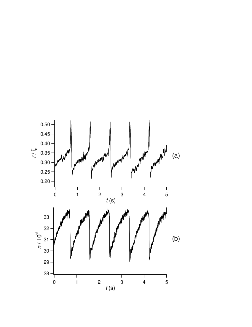
Figure 2: Experimental record of the time evolution of the cloud when C_P instabilities occur. In (a), CM motion $r$; in (b) population $n$. $\Delta_{0}=-1.40$, $I_{1}=10$ and $I_{r}ep=1.2$ mW/cm².

C₁ instabilities, illustrated in Fig. 3, corresponds to a motion of the cloud very similar to that of C_P instabilities. Indeed, $r$ exhibits the same behavior along the same type of cycle, covered with two different time scales separated by one order of magnitude. The main difference comes from the erraticity of the motion, which is no more periodic: indeed, although the basic pattern of the motion remains the same cycle, the duration of each cycle fluctuates. From the dynamical point of view, it is convenient use the return time between two cycles, which, in chaotic dynamics, is known to be a relevant variable of the systemRT . The $r$ return time is constant in periodic motions (C_P instabilities), while it is fluctuating in C₁ instabilities. The $n$ return time is also varying in C₁ instabilities, but other differences as compared to C_P regime appear. In particular, the ratio between the fast and slow stages of the dynamics fluctuates, so that for some periods, the two stages occur with a comparable time scale. In short, C₁ instabilities appears as C_P instabilities, in which noisy fluctuations appear, essentially on the return time.

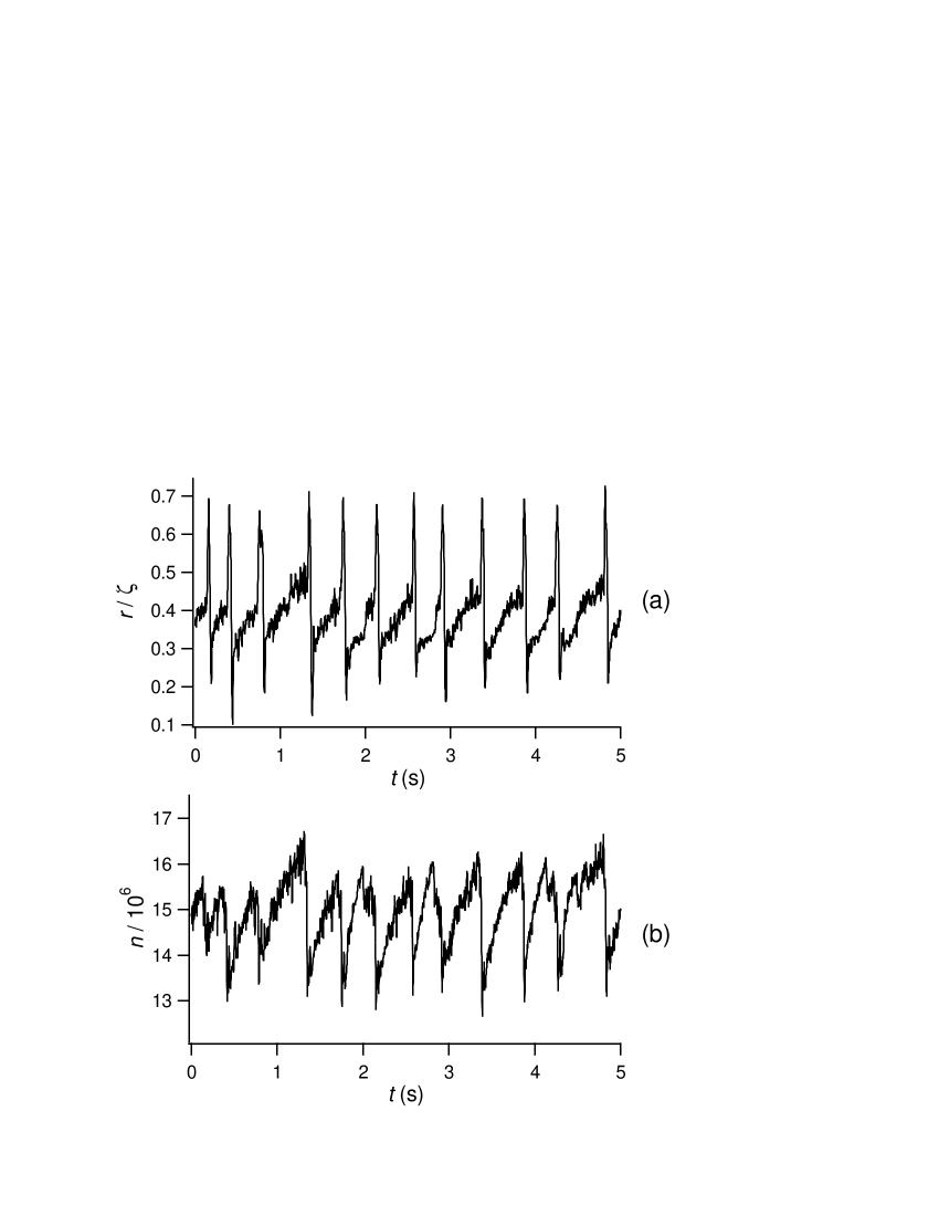
Figure 3: Experimental record of the time evolution of the cloud when C₁ instabilities occur. In (a), CM motion $r$; in (b) population $n$. $\Delta_{0}=-0.85$, $I_{1}=10$ and $I_{r}ep=1.2$ mW/cm².

With C_S instabilities (Fig. 4), any periodicity has disappeared from the behavior of both $r$ and $n$. Not only the return time is fluctuating, but also the amplitude of the cycles changes with time. In fact, speaking of cyclic behavior in the present case is excessive, except that the basic pattern of the motion keeps similarities with the cycle of C_P instabilities, in particular the two stages with different time scales. However, even the motion cycle is irregular, with secondary fast oscillations appearing during the slow stage, while the amplitude of the $n$ cycle can fluctuate in a ratio of 1:5.

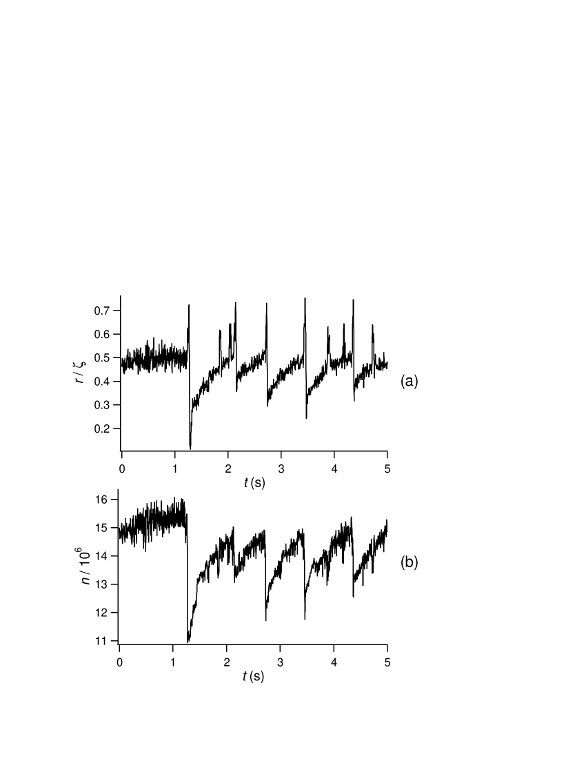
Figure 4: Experimental record of the time evolution of the cloud when C_S instabilities occur. In (a), CM motion $r$; in (b) population $n$. $\Delta_{0}=-0.75$, $I_{1}=10$ and $I_{r}ep=1.2$ mW/cm².

The differences between the three C behaviors are particularly well illustrated by the power spectrum of $r$, as shown in Fig. 5. The spectrum of C_P instabilities exhibits a first large and narrow peak, at about 1 Hz, corresponding to the main period of the signal, followed by a series of harmonics (Fig. 5a). These harmonics are a signature of the second time scale, much faster than the basic period, which appears in the fast oscillation of $r$. For C₁ instabilities (Fig. 5b), the first peak remains, demonstrating that the signal remains essentially periodic. However, the regularly spaced harmonics have disappeared, but high frequency components remain. They are distributed erratically, but have globally a larger weight than in C_P instabilities. Finally, for C_S instabilities, the main frequency component has decreased drastically, and the spectrum may rather be considered as a wide spectrum, as those observed in chaotic or stochastic signals. Unfortunately, it is impossible to distinguish between these two possibilities through the spectrum analysis of the behavior. To do so, it is necessary to turn to more powerful techniques, such as the reconstruction of the attractor of the dynamics.

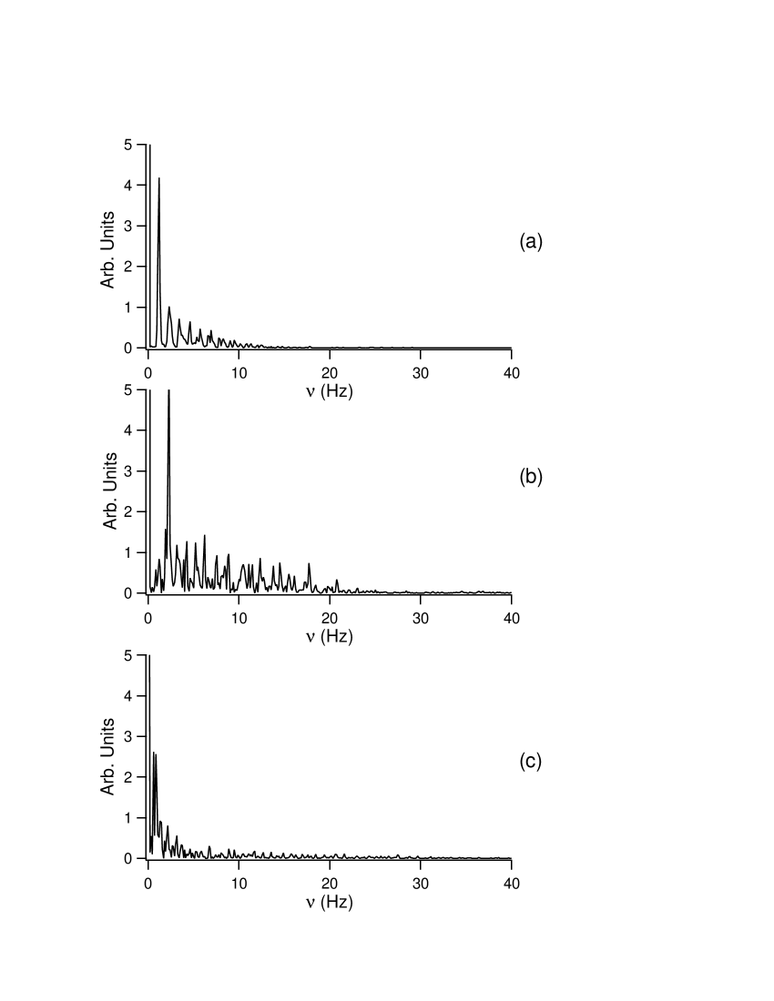
Figure 5: Spectra of the CM location time evolution in case of C instabilities. Figures (a), (b) and (c) correspond respectively to Fig. 2a, Fig. 3a and Fig. 4a.

Indeed, the MOT is a dissipative system, and any deterministic behavior lies in the phase space on an attractor. In the case of deterministic chaos, this attractor is complex, but has usually a structured shape, easily recognizable. On the contrary, if the behavior is dominated by noise, there is no attractor, and the trajectories fill the whole phase space. The reconstruction of the attractor of a system from experimental time series is a well mastered operation. It can be performed following several methods (delays, derivatives), and needs usually additional steps, as the plot of the Poincaré section. In the present case, the use of return times is particularly well adapted, as it appears as one of the main properties of the behavior. The return time diagram, which is equivalent to a Poincaré section, consists in plotting the return time between cycles $n$ and $n+1$, as a function of the return time between the cycles $n-1$ and $n$RTD . The Poincaré section is a cross-section of the attractor, and has a dimension decreased of one unit as compared to the attractor. Thus, first return time diagrams of C_P instabilities give just a point, as expected from a cyclic behavior. Fig. 6 shows the first return time diagram in the case of C₁ instabilities. It is a good illustration of all the return times diagram we have obtained for C₁ and C_S instabilities: points appear to be distributed randomly in the phase space, without any structure. Thus we can conclude that the behavior is either high-dimensional deterministic chaos, or a stochastic dynamics. From the point of view of the model discussed below, these two hypotheses are equivalent, as the model includes only three degrees of freedom.

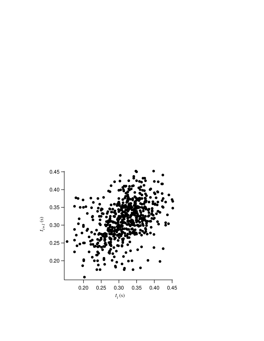
Figure 6: Typical first return time diagram, obtained from a time series of 200 s with $\Delta_{0}=-1$, $I_{1}=16$ and $I_{rep}=7.5$ mW/cm².

The links between the different C regimes appear clearly when one looks at the dependence of the behavior versus the different control parameters, and in particular $I_{1}$ and $\Delta_{0}$. It was already shown in bruit2002 that for small trap beam intensity $I_{1}$ (typically $I_{1}\leq 3$), the atomic cloud exhibits only S instabilities. When $I_{1}$ is increased, S instabilities still exist, but they are progressively superseded by C instabilities. The appearance of C instabilities occurs progressively, at the cost of S instabilities. For intermediate values of $I_{1}$, both types of instabilities exist. Their typical distribution versus $\Delta_{0}$ is illustrated in Fig. 7: far from resonance, the cloud is stable; as the resonance is approached, S instabilities appear for a detuning $\Delta_{0}=\Delta_{1}$. Then C instabilities appear in $\Delta_{2}>\Delta_{1}$. If the detuning is still increased, C instabilities disappear in $\Delta_{3}$ at the benefit of a stable behavior. Finally, the cloud vanishes in $\Delta_{4}$. As $I_{1}$ is increased, the interval $\delta_{23}=\Delta_{3}-\Delta_{2}$ where C instabilities occur, increases at the cost of the width $\delta_{12}=\Delta_{2}-\Delta_{1}$ where S instabilities occur, while the total unstable interval $\delta_{13}=\Delta_{3}-\Delta_{1}$ remains more or less constant. When C instabilities merge for $I_{1}=4I_{S}$, they appear on a narrow interval $\delta_{23}\gtrsim 0$ (Fig. 8). This interval increases rapidly until $I_{1}=7.5I_{S}$ and $\delta_{23}=0.8$. For $I_{1}>7.5I_{S}$, $\delta_{23}$ increases more slowly, to reach the value of $\delta_{23}=1$ in $I_{1}=20I_{S}$. The value of $\delta_{23}$ depends also on the other parameters of the system. Fig. 8b illustrates, as an example, how it depends on the repumper intensity $I_{rep}$, at given $I_{1}$: $\delta_{23}$ varies from 0 for $I_{rep}\simeq 0.4$ mW/cm² to $1$ for $I_{rep}>1$ mW/cm².

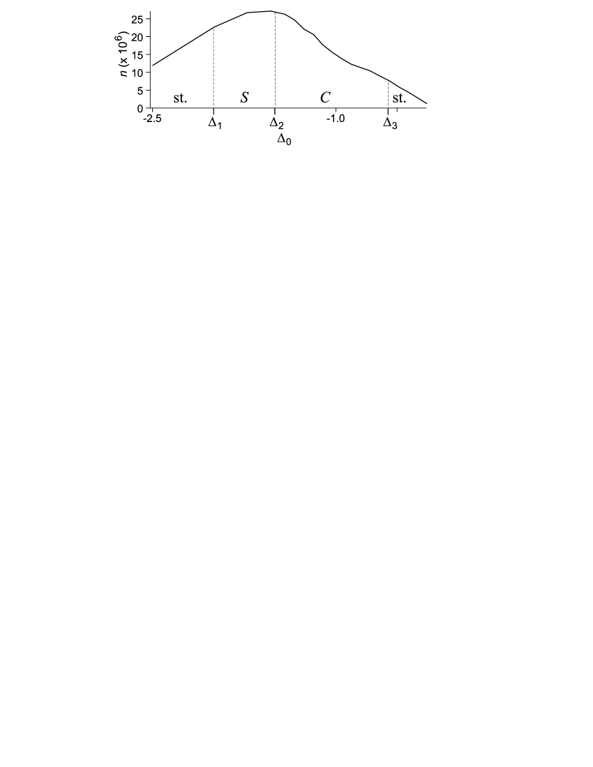
Figure 7: This figure illustrates the evolution of the behavior as a function of the detuning for $I_{1}=6.8$ and $I_{rep}=1.5$ mW/cm²; The full line reports the population, while the dashed lines separate the domain of different behaviors: st. stands for stable, S (C) for $S$ ($C$) instabilities.

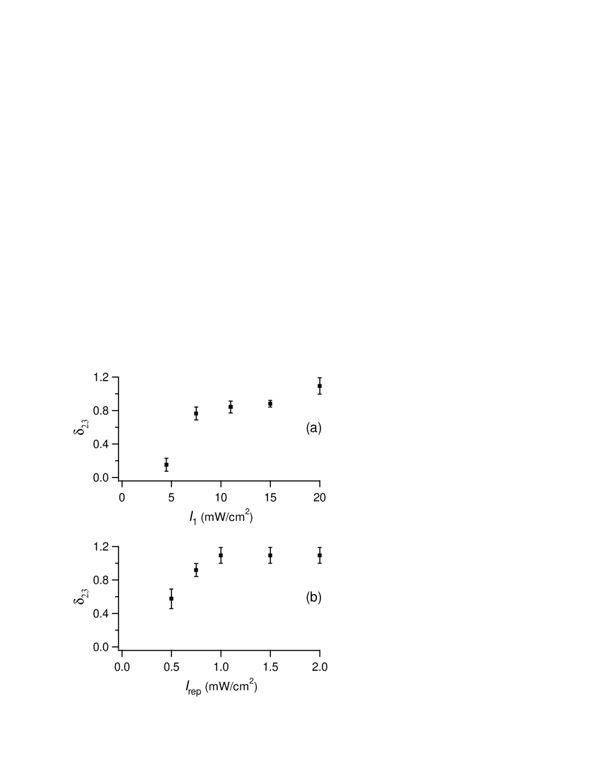
Figure 8: Width $\delta_{23}$ of the C instabilities area as a function of (a) the MOT intensity $I_{1}$ and (b) the repumper intensity $I_{rep}$. In (a), $I_{rep}=1.5$ mW/cm², and in (b), $I_{1}=18$

Between $\Delta_{2}$ and $\Delta_{3}$, the different types of C instabilities appear, following a constant scenario. In $\Delta_{2}$, when they merge abruply from a stable or S behavior, they are C_P instabilities, and as $\Delta_{0}$ is increased, they transform successively in C₁, then C_S instabilities in $\Delta_{3}$. The evolution is continuous, without abrupt changes, and the C₁ and C_S instabilities appear rather as two different levels of deterioration of C_P instabilities by noise. From this point of view, C₁ instabilities appear as an intermediate stage between C_P and C_S instabilities where noise destroys only the periodicity, without affecting the cycle itself.

The amplitude of the oscillations, of the order of 100 $\mu$m in $\Delta_{2}$, is much larger than that of the S instabilities they merge from, which is typically 30 $\mu$m. This is an interesting result, because in the most usual bifurcations between stable and cyclic behaviors, as the Hopf bifurcation, the cycle merges progressively from a zero amplitude. Such an atypical behavior can be considered as a signature of the present system, and must be retrieve in the behavior predicted by the model.

When $\Delta_{0}$ is increased from $\Delta_{2}$, this amplitude still increases, such that the oscillations reach a 100% contrast in $z$ and an amplitude of 40% in $n$ (Fig. 4). Simultaneously, the instabilities frequency remains almost constant, as illustrated on Fig. 9 for different values of the intensity $I_{1}$. The frequency reported here is the main frequency component for C_P and C₁ instabilities, and the inverse of a mean return time for C_S instabilities. It appears clearly that at given $I_{1}$, the main frequency does not change between $\Delta_{2}$ and $\Delta_{3}$. This is another interesting result, also very untypical in dynamical systems, where the nonlinear resonance frequencies usually depend stricly on the parameters.

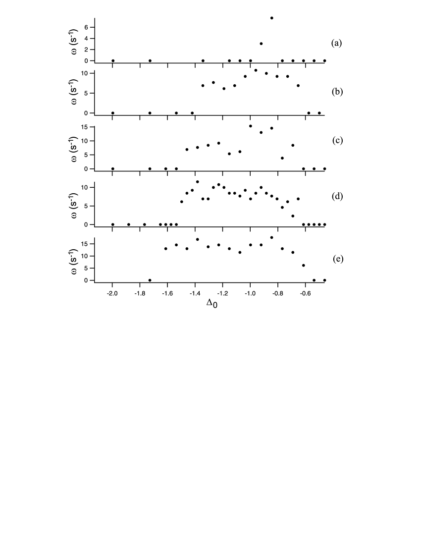
Figure 9: Experimental evolution of the angular frequency of the instabilities as a function of the detuning for different values of the beam internsity: in (a), $I_{1}=4.1$; in (b), $I_{1}=6.8$; in (c), $I_{1}=10$; in (d), $I_{1}=13.6$; in (e), $I_{1}=18$. $I_{r}ep=1.5$ mW/cm² in all cases.

To conclude this section, let us summarize the main characteristics of the C instabilities. Three types of behaviors have been identified, depending on their degrees of stochasticity: the C_P instabilities are strictly periodic, the C₁ instabilities remain cyclic, but are no more periodic, while finally, the C_S are neither cyclic, nor periodic. However, this last regime differs drastically from S instabilities described in bruit2002 , by their amplitude, and by a residue of the cycles they merge from. C behaviors appear abruptly, with a non-zero amplitude, and their main frequency appears to be independent from the detuning.

4 Model

To determine the origin and the exact nature of the instabilities observed in the experiments, we need to build a model able to reproduce also the complex stochastic dynamics observed in bruit2002 . Thus it is logical to use the model introduced in InstDet and described in details in bruit2002 . It is a 1D model based on the shadow effect induced by the intensity gradients produced by the absorption of the trapping laser beams in the cloud shadow ; dalibard . The aim of this model is not to reproduce as finely as possible the experimental system, but on the contrary to be as simple as possible, enlighting the fundamental mechanisms leading to the instabilities. In its final form, the model reduces to a set of three autonomous equations, i.e. three equations not depending explicitely on time. This is important, as it is the minimum number of degrees of freedom necessary to generate complex dynamics, in particular deterministic chaos. The model writes:

$$\frac{dZ}{dt} = V\frac{v_{r}}{z_{0}}$$ (1a)

$$\frac{dV}{dt} = \frac{1}{Mv_{r}}F_{T}$$ (1b)

$$\frac{dN}{dt} = B\left(1-Z^{2}-N\right)$$ (1c)

where $Z=z/z_{0}$, $V=v/v_{r}$ and $N=n/n_{0}$ are the reduced variables of the MOT. $z$ and $v$ is the location and the velocity of the center of mass of the cloud along the unique axis $z$ of the system, while $n$ is the number of atoms inside the cloud. $z_{0}$ is a phenomenological size introduced to take into account the transverse distribution of the trap laser beams, $v_{r}$ is the recoil velocity ($v_{r}=\hbar k/m$), and $n_{0}$ is the equilibrium population of atoms in the cloud. The origin of $z$ coincides with the “trap center”, that is, the zero of the magnetic field. $B$ is the population relaxation rate, $M$ the mass of the cloud and $F_{T}$ the global force exerted on the atoms by the two counterpropagating beams. To evaluate $F_{T}$, we assume a multiple scattering regime, i.e. a constant atomic density $\rho$ in the cloud. Then $F_{T}$ is deduced from the equations of propagation of the beams inside the cloudbruit2002 .

Most of the theoretical parameters are the exact counterpart of the experimental parameters, as e.g. the magnetic field gradient or the beam intensities. In this case, we used in the model the same values as those of Table 1. It is not the case for all parameters, either because of the simplicity of the model or because they cannot be measured easily in the experiment. In particular, $n_{0}$ and $\rho$ cannot be accurately evaluated in the experiments. Thus in the simulations, they are fixed at experimental averaged values, and they have been varied on a wide range to check their value is not critical. Finally, to perform the comparison between the experiments and the present model, we sometimes need to study the behavior of the system when noise is added. This has been done in the same way as in bruit2002 , by adding gaussian white noise on $I_{1}$. Tab. 2 summarizes the parameters used in the following.

Table 2: Parameters used in the numerical simulations. The range corresponds to the interval explored numerically, while the other sets refer to most of the results presented in this paper.

	range	set #1	set #2
$G$ (Gcm-1)	$14$	$14$	$14$
$B$ (s-1)	$3\leq B\leq 30$	$3$	$3$
$I_{1}$	$2\leq I_{1}\leq 30$	25	30
$\rho$ (cm-3)	$10^{10}\leq\rho\leq 3\times 10^{10}$	$2\times 10^{10}$	$2\times 10^{10}$
$S$ (m2)	$10^{-6}\leq S\leq 3\times 10^{-6}$	$10^{-6}$	$10^{-6}$
$z_{0}$ (m)	$10^{-2}\leq z_{0}\leq 3\times 10^{-1}$	$3\times 10^{-2}$	$3\times 10^{-2}$
$n_{0}$	$10^{7}\leq n_{0}\leq 10^{9}$	$10^{8}$	$6\times 10^{8}$
$\Delta_{0}$	$5\leq\Delta_{0}\leq-0.5$	$-1.5$	$-1.5$

5 Stationary solutions

The model obtained above is described by a set of three autonomous equations, and thus could exhibit complex behaviors, including periodic and chaotic oscillations, able to explain the dynamics observed experimentally. To know if such a complex dynamics occurs effectively with our parameters, we need first to evaluate the stability of the stationary solutions, and thus to calculate the stationary solutions themselves. This work has already been partially presented in bruit2002 , for stable stationary solutions, while we are interested here by unstable stationary solutions. However, for sake of clarity, we recall here some of the general results given in bruit2002 , before to start the analysis of the unstable stationary solutions.

The three stationary solutions $Z_{s}$, $V_{s}$ and $N_{s}$ are given by Eq.1, when the left sides are put to zero. As discussed in bruit2002 , $V_{s}$ and $N_{s}$ can be deduced easily from $Z_{s}$, and thus the discussion is reduced to that of $Z_{s}$, the equation of which can be resolved numerically. The global shape of $Z_{s}$ is illustrated in Fig. 10, where it is plotted as a function of $\Delta_{0}$ and $n_{0}$. The basic characteristic of this diagram is the fold in the stationary solutions, due to several abrupt slope changes. The shape of the fold depends on the parameters, in particular on $n_{0}$. Fig. 11 shows four examples corresponding to a situation leading to basically different atomic dynamics. For $n_{0}=0.5\times 10^{8}$ (fig. 11a), $Z_{s}$ increases smoothly with $\Delta_{0}$ (i.e. $N_{s}$ decreases slowly). For $\Delta_{0}\simeq 0.1$ (and thus outside the graph), the cloud vanishes through a narrow bistable cycle, where $Z_{s}$ jumps abruptly from a value of the order of $0.2$ to a value close to $1$. As $n_{0}$ increases, this bistable cycle appears for smaller $Z_{s}$ (and thus larger $N_{s}$), and becomes physically significant. Fig. 11b shows $Z_{s}$ for $n_{0}$ $=2.5\times 10^{8}$ and a bistable cycle for $-0.3\lesssim\Delta_{0}\lesssim-0.25$. If $n_{0}$ is further increased, the bistable cycle disappears, but it remains a fold corresponding to two abrupt slope changes of $Z_{s}$ versus $\Delta_{0}$ (fig. 11c, $n_{0}$ $=3.4\times 10^{8}$). If $n_{0}$ is still increased, the fold remains, but it becomes smoother (Fig. 11d for $n_{0}=$ $4\times 10^{8}$).

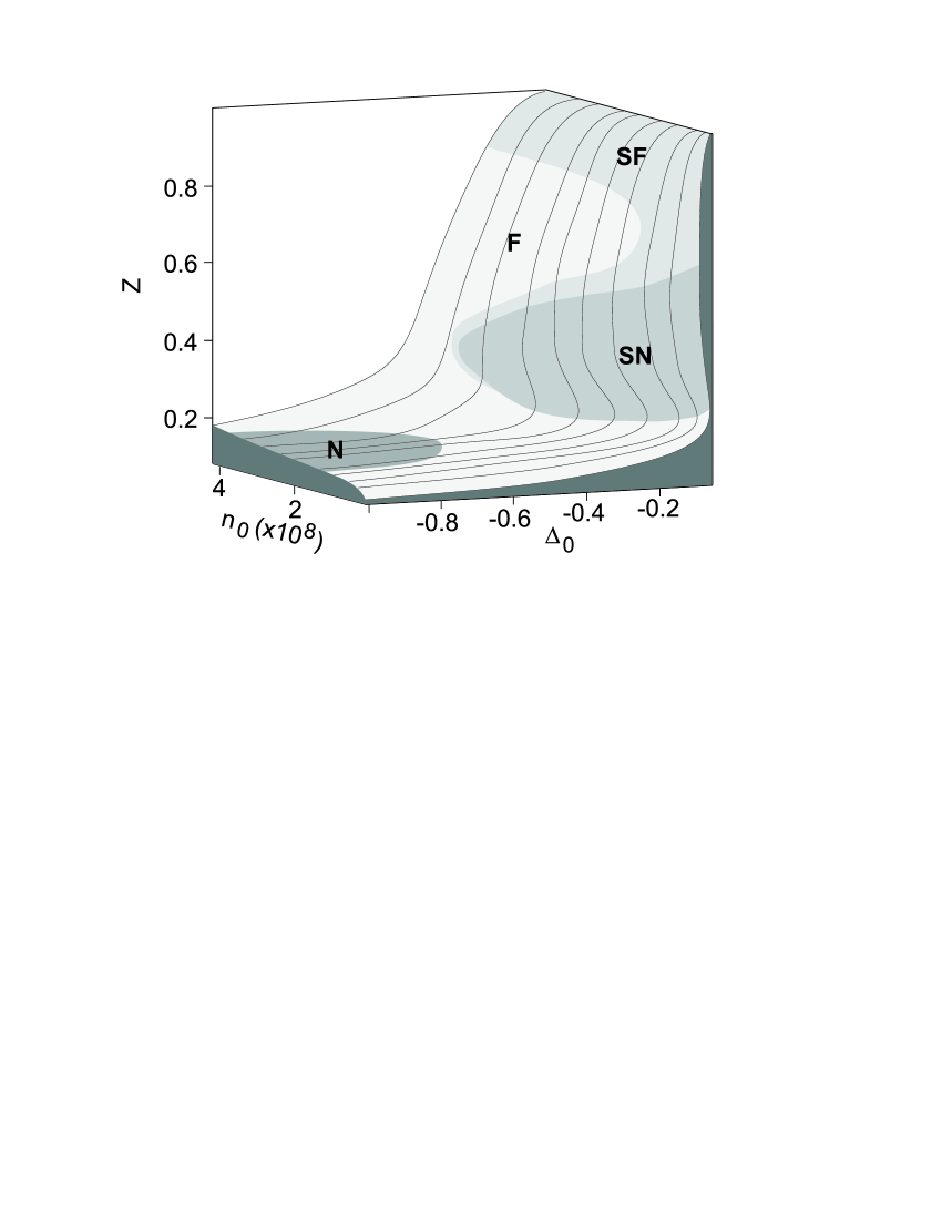
Figure 10: Stationary solutions of equations 1 versus $n_{0}$ and $\Delta_{0}$. The figure represents $Z_{s}$. Other parameters correspond to the set #1 given in table 2. N, F, SN and SF zones (each corresponding to different level of greys) describes the nature of the fixed point associated with the stationary solution: stable Node, stable Focus, Saddle Node and Saddle Focus.

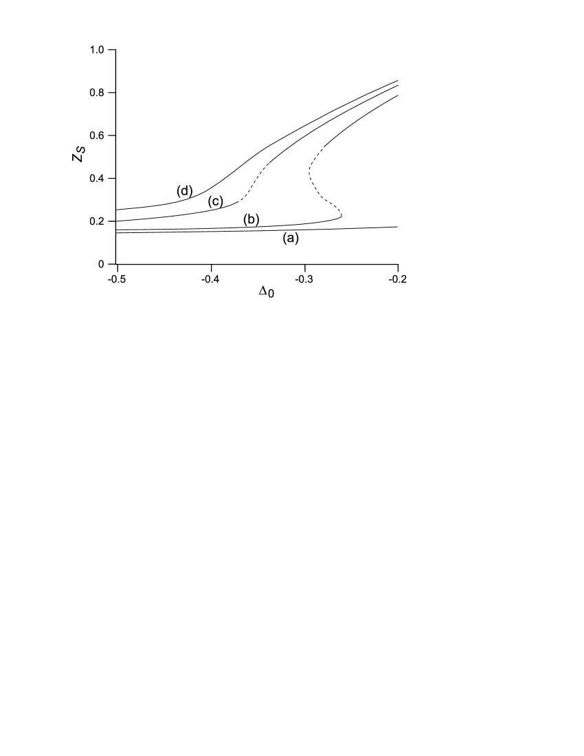
Figure 11: Evolution as a function of the detuning of the stationary solution $Z_{s}$ of equations 1. The full (resp. dashed) line corresponds to a stable (resp. unstable) solution. In (a), $n_{0}=0.5\times 10^{8}$; in (b) $n_{0}=2.5\times 10^{8}$; in (c), $n_{0}=3.4\times 10^{8}$; in (d), $n_{0}=4\times 10^{8}$ Other parameters correspond to the set #1 of Table 2

The results of the linear stability analysis have been detailed in bruit2002 . It was shown that the stability and nature of the stationary solutions evolve along the fold. In particular, the solutions are unstable not only on the central branch of the bistable cycle, as it is usual, but also on the upper branch of the bistable cycle, and even when there is no bistability. This is illustrated in Fig. 11, where the unstable solutions are plotted in a dashed line. As we deal here with deterministic instabilities, the interesting situation corresponds to Fig. 11c, where the unique stationary solution is unstable on the fold. Note the difference with the cases studied in bruit2002 , where the stationary solution is also unique, but stable. In the present case, as no stable solution exists, the system exhibits necessarily deterministic instabilities.

Fig. 12 details the changes in the eigenvalues in this situation. Outside the fold (i.e. $\Delta_{0}<\Delta_{1}$ or $\Delta_{0}>\Delta_{4}$), $Z_{S}$ is stable, with one real eigenvalue $\lambda_{r}$ and two complex conjugate eigenvalues $\lambda\pm i\omega$: the fixed point associated to the stationary solution in the phase space is a stable focus (F zone in Fig. 10). The real numbers $-\lambda_{r}$ and $-\lambda$ are the damping rates of the stationary solution, and $\omega$ its eigenfrequency. The transition from stable focus solution to unstable saddle focus solution occurs in $\Delta_{1}$ and $\Delta_{4}$, through a Hopf bifurcation, where $\lambda=0$ and $\omega\neq 0$. As it is usual for such a bifurcation, we expect to observe, on the unstable side, a cloud moving on a limit cycle with a frequency $\omega$, i.e. in the present case of the order of 200 s^-1 (30 Hz) for both Hopf bifurcations. Another transition, from a saddle focus solution to a saddle node solution, occurs in $\Delta_{2}$ and $\Delta_{3}$, when $\omega$ vanishes. The behavior here cannot be deduced from the stationary solutions, and numerical simulations are necessary. Deterministic instabilities are expected to occur between $\Delta_{1}$ and $\Delta_{4}$. In all other areas, the stationary solutions are stable, and therefore, deterministic instabilities cannot occurbruit2002 . In the next section, we detail the results of numerical simulations performed in the unstable area.

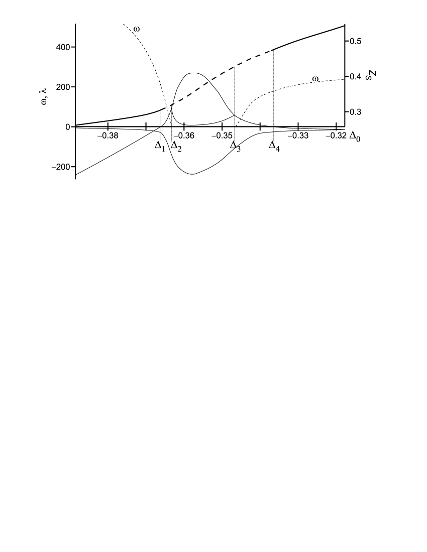
Figure 12: Evolution as a function of the detuning of the stationary solution $Z_{S}$ and its eigenvalues, for the parameters of Fig. 11c. The stationary solution is given through the full (stable) and dashed (unstable) bold lines. The dashed line noted $\omega$ represents the imaginary part of the complex eigenvalues, while the full lines correspond to the real part of the three eigenvalues. The full line remaining negative corresponds to the eigenvalue which is real everywhere.

However, before to discuss in detail the dynamical behaviors predicted by the model in the different situations, let us look at the influence of the other parameters on the stationary solutions. As discussed in the previous section, we must distinguish between theoretical parameters with an exact experimental counterpart, as $I_{1}$, for which the comparison with experiments is direct, from those without an exact experimental counterpart, for which the analysis is more delicate. It is in particular the case for $n_{0}$ and $\rho$, which are both linked to $I_{rep}$ and the vapour pressure. Finally, the influence of $B$ and $z_{0}$ should be checked, as their experimental determination is unprecise.

Fig. 13 illustrates the role of the $I_{1}$ value on the behavior of the cloud: it represents the stationary solution $Z_{S}$ versus the detuning, for different values of the intensity. The figure shows that $I_{1}$ acts as $n_{0}$ on $Z_{S}$: an increase of $I_{1}$ makes the fold steeper, and eventually leads to bistability. However, some more subtle changes occur, as illustrated by Fig. 14, where $Z_{S}$ have been plotted as a function of $\Delta_{0}$ for different values of $n_{0}$, as in Fig. 11, but for a smaller intensity. In these new conditions, the intermediate area between the stable fold and bistability, where the stationary solution is unique and unstable, has almost disappear. This result may be generalized: in the simulations, we observed that the area corresponding to an unstable unique solution disappears for small intensities (typically $I_{1}<10$). This result is in agreement with the experimental observation that C instabilities exist only for large intensities.

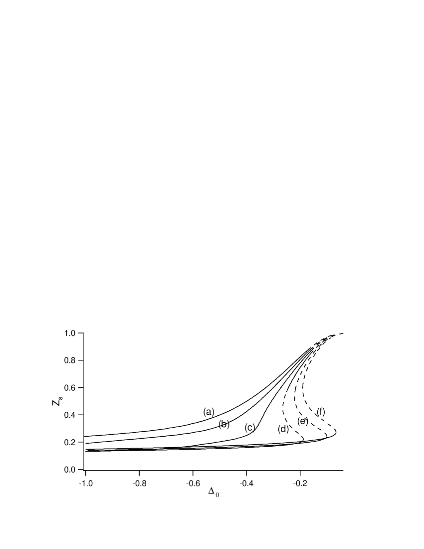
Figure 13: Evolution as a function of the detuning of the stationary solution $Z_{s}$ of equations 1 for different values of the intensity $I_{1}$. The full (resp. dashed) line corresponds to a stable (resp. unstable) solution. In (a), $I=10$; in (b) $I=15$; in (c), $I=20$; in (d), $I=25$; in (e), $I=30$; in (d), $I=35$. Other parameters correspond to the set #1 of Table 2, with $n_{0}=2\times 10^{8}$.

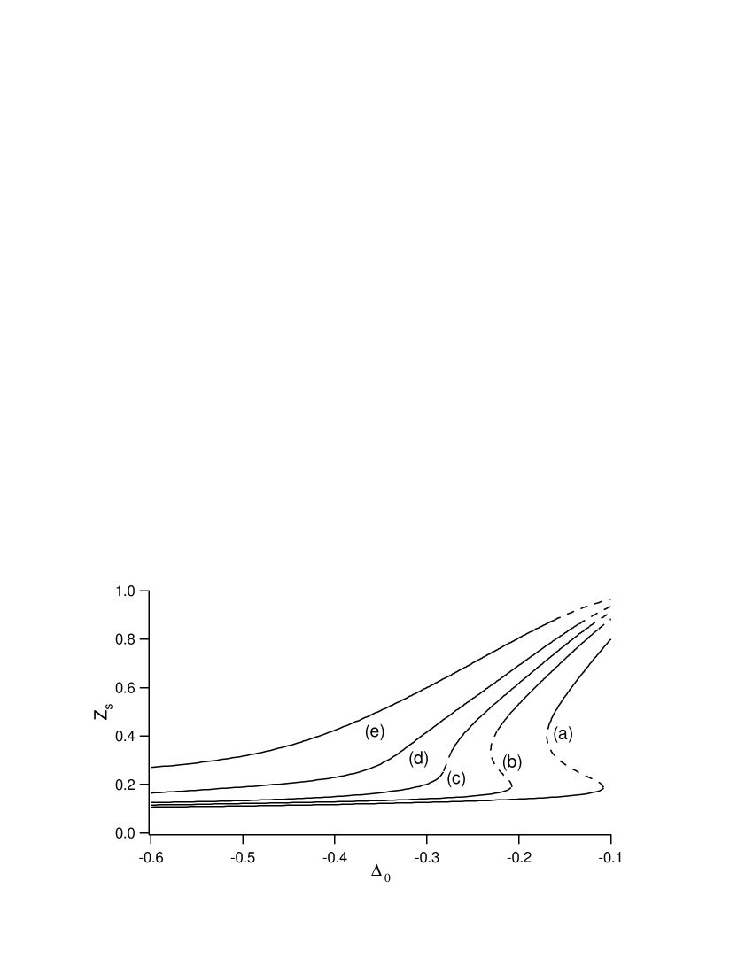
Figure 14: Evolution as a function of the detuning of the stationary solution $Z_{s}$ of equations 1 for different values of $n_{0}$ and a smaller intensity than in Fig. 11. The full (resp. dashed) line corresponds to a stable (resp. unstable) solution. In (a), $n_{0}=0.25\times 10^{8}$; in (b) $n_{0}=0.5\times 10^{8}$; in (c), $n_{0}=0.7\times 10^{8}$; in (d), $n_{0}=1\times 10^{8}$; in (e), $n_{0}=2\times 10^{8}$. Other parameters correspond to the set #1 of Table 2, with $I_{1}=15$.

The atomic density value used in the present simulation is $\rho=2\times 10^{10}\mathop{\rm cm}^{-3}$, which represents an average of the density we measured experimentally. To evaluate the influence of this value on the predicted behavior, we have plotted in Fig. 15 the evolution of $Z_{S}$ for different values of $\rho$. As for $n_{0}$ and $I_{1}$, the $Z_{S}$ curve evolves from an almost flat dependence for large $\rho$, towards bistability for small $\rho$, with an intermediate SF zone. This can appear as surprising, because it seems to mean that nonlinear behaviors, corresponding to the bistable cycle, need a small atomic density. In fact, this reasoning is false, because it does not take into account the role of the other parameters, in particular $n_{0}$, which is able to compensate for the variation of $\rho$. For example, fig. 16 shows the $\left(\Delta_{0},n_{0}\right)$ diagram for a smaller $\rho$ value than in Fig. 11: it has the same properties as that in fig. 11, except that the population are much larger. However, one remarks slight differences, in particular a small decreasing of the $Z$ values, and first of all a small decreasing of the SF zone width. This is another general result: in the simulations, when the atomic density is decreased, the $Z_{s}$ curves globally flatten, so that the fold becomes less steep. Thus all instabilities disappear for very small densities. This is in agreement with the experimental results illustrated in Fig. 8b, where the unstable interval width is reported as a function of $I_{rep}$: the instabilities disappear for small $I_{rep}$, i.e. when the efficiency of the repumper – and thus the atomic density – decreases.

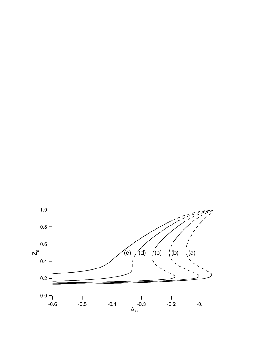
Figure 15: Evolution as a function of the detuning of the stationary solution $Z_{s}$ of equations 1 for different values of the atomic density. The full (resp. dashed) line corresponds to a stable (resp. unstable) solution. In (a), $\rho=1\times 10^{10}$ cm^-3; in (b), $\rho=1.5\times 10^{10}$ cm^-3; in (c), $\rho=2\times 10^{10}$ cm^-3; in (d), $\rho=2.5\times 10^{10}$ cm^-3; in (e), $\rho=3\times 10^{10}$ cm^-3. Other parameters correspond to the set #1 of Table 2, with $n_{0}=2\times 10^{8}$ and $I_{1}=25$.

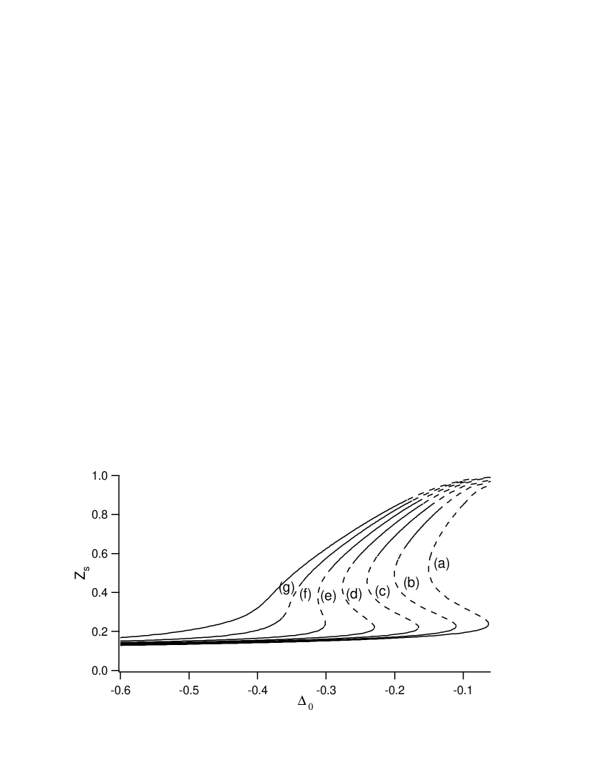
Figure 16: Evolution as a function of the detuning of the stationary solution $Z_{s}$ of equations 1 for different values of $n_{0}$ and a smaller atomic density than in Fig. 11. The full (resp. dashed) line corresponds to a stable (resp. unstable) solution. In (a), $n_{0}=2\times 10^{8}$; in (b) $n_{0}=4\times 10^{8}$; in (c), $n_{0}=6\times 10^{8}$; in (d), $n_{0}=8\times 10^{8}$; in (e), $n_{0}=1\times 10^{9}$; in (f), $n_{0}=1.2\times 10^{9}$; in (g), $n_{0}=1.4\times 10^{9}$. Other parameters correspond to the set #1 of Table 2, with $\rho=1\times 10^{10}$ cm^-3.

As detailed in bruit2002 , the value of $z_{0}=3\mathop{\rm cm}$ used in the experiments has been evaluated from the trap beam waist, taking into account the beam intensity as compared to the saturation intensity. As for $\rho$, we want to evaluate how critical is this choice by plotting $Z_{S}$ versus $\Delta_{0}$ for different values of $z_{0}$ (Fig. 17). It appears clearly that a decreasing of $z_{0}$ corresponds to a shift of the fold and the bistable cycle towards resonance. Thus, for $z_{0}$ values smaller than 3 cm, the discrepancy between simulations and experiments increases quantitatively, as instabilities will appear at smaller detuning. For values smaller than 1 cm, the change is drastic, as the SF and bistable zones, and thus instabilities, disappear. On the contrary, for larger $z_{0}$, the bistable cycle widens and shifts off resonance.

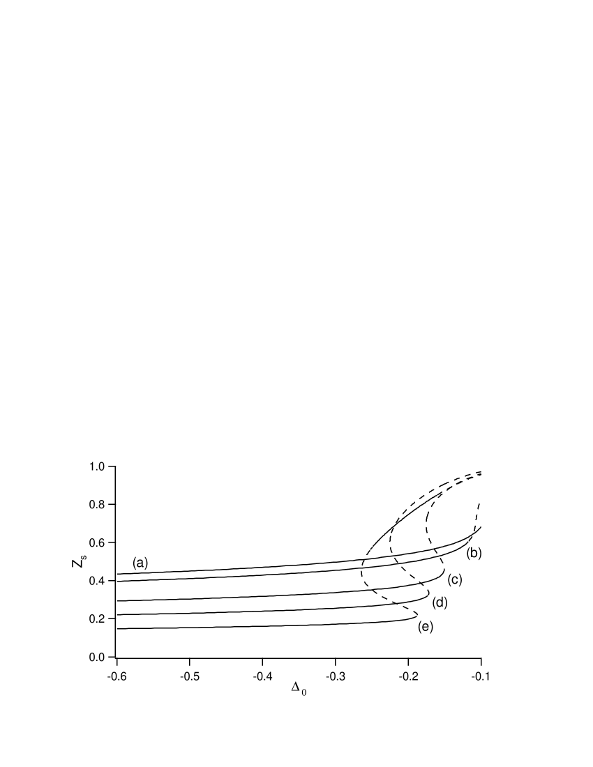
Figure 17: Evolution as a function of the detuning of the stationary solution $Z_{s}$ of equations 1 for different values of $z_{0}$. The full (resp. dashed) line corresponds to a stable (resp. unstable) solution. In (a), $z_{0}=1$ cm; in (b), $z_{0}=1.1$ cm; in (c), $z_{0}=1.5$ cm; in (d), $z_{0}=2$ cm; in (e), $z_{0}=3$ cm. Other parameters correspond to the set #1 of Table 2, with $n_{0}=2\times 10^{8}$ and $I_{1}=25$.

The last parameter to be considered is $B$. This parameter appears to be not critical at all, and in particular, a change from e.g. $B=5\mathop{\rm s}^{-1}$ to $B=1\mathop{\rm s}^{-1}$ does not change in a noticeable way the values of $Z_{S}$. The main change concerns the smaller real eigenvalue, which takes typically the value of $-B$. However, this eigenvalue plays a minor role in the dynamics, as it remains always real negative, and thus this change has a negligible effect on the dynamics.

It appears from the above analysis that the existence of the unstable area does not depend critically on the values of $n_{0}$, $I_{1}$, $\rho$, $z_{0}$ and $B$. In particular, the relative poor accuracy in the knowledge of the experimental values of some parameters, as $n_{0}$, $\rho$ or $z_{0}$, does not appear as a limitation in the above study, because a change of some tens of percents around the default values used in the simulations does not alter the results. The numerous approximations at the origin of the model lead probably to larger errors.

6 The unstable fold: deterministic instabilities

As shown in the previous section, it exists a range of parameters where the stationary solution is unique and unstable. Such a situation leads inevitably to deterministic instabilities, with shape and characteristics obtained through numerical simulations of the model for the corresponding sets of parameters. In the present section, we discuss the behavior obtained by such simulations, in a situation similar to Figs 11c and 12, but for a slightly different set of parameters (set #2 of Tab. 2). Fig. 18 shows for these conditions the evolution of the eigenvalues as a function of the detuning. The sequence is identical to that followed in Fig. 12, but the unstable zone is wider. Starting off resonance, a Hopf bifurcation occurs in $\Delta_{1}$. In $\Delta_{2}$, the eigenvalues become real, and thus the eigenfrequency disappears, until $\Delta_{3}$, where two eigenvalues are again complex. Finally, a second Hopf bifurcation occurs in $\Delta_{4}$, and the stationary solutions become stable again.

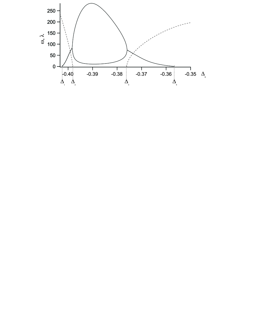
Figure 18: Evolution as a function of the detuning of the eigenvalues of the stationary solutions. The full line, which is a plot of the real part $\lambda$ of the eigenvalues when they are positive, put in evidence two bifurcations, in $\Delta_{1}=-0.4024$ and $\Delta_{4}=-0.3566$. The dashed line represents the corresponding imaginary part $\omega$ (i.e. the eigenfrequencies). The eigenvalues are real between $\Delta_{2}=-0.3981$ and $\Delta_{3}=-0.3760$. Parameters corresponds to the set #2 of Tab. 2.

6.1 The behavior in the vicinity of the Hopf bifurcation

To understand the origin of the C instabilities, we have studied in detail the behavior of the model in the close vicinity of the H₁ Hopf bifurcation, by varying $\Delta_{0}$ slightly above $\Delta_{1}$. The expected scenario has been extensively described in the litteratureRT . On the left of H₁, the stationary solution is stable, and thus the behavior is stationary. In H₁, the solution becomes unstable, but a limit cycle merges from the unstable fixed point: the behavior becomes periodic, with a zero amplitude in H₁, and a frequency corresponding to the relaxation frequency of the unstable solution. On the right of the bifurcation, the amplitude of the oscillations grows, while the frequency remains the same as the eigenfrequency in the vicinity of H₁. Usually, when the control parameter is increased from H₁, the cycle shape changes progressively, while the interval between the oscillation and relaxation frequencies becomes larger. This standard scenario is absolutely not followed by the present model. On the contrary, several abrupt changes in the behavior occur in a very narrow interval of $\Delta_{0}$, leading from a classic regular limit cycle to the C_P instabilities.

In H₁ appears, as expected, a limit cycle. Figs. 19 and 20 show the evolution of this limit cycle on the unstable side of the bifurcation between $\Delta_{1}$ and $\Delta_{1}^{\prime}=-0.4010$. Note that the explored interval is so narrow ($1.3\times 10^{-3}$) that an experimental observation of the described phenomena cannot be considered. Following the $Z$ coordinate, the cycle amplitude grows rapidly to reach a value of typically $10\%$ of $Z_{S}$, while the amplitude on $N$ remains very small ($0.1\%$ of $N_{S}$). The cycle remains relatively well centered on $Z_{S}$, but is shifted compared to $N_{S}$, such that $N_{S}$ is well outside the cycle. This is not an exceptional situation, as it simply means that the basin of attraction of the cycle is curved in the vicinity of the unstable fixed point. Another characteristics of the limit cycle is its frequency, which remains of the order of magnitude of the eigenfrequency. For example, for $\Delta_{0}=-0.4015$ (Fig. 19c), the behavior frequency is 30 Hz, for an eigenvalue of 27 Hz. Thus the global behavior in the interval $(\Delta_{1},\Delta_{1}^{\prime})$ appears to be the usual one in the vicinity of a Hopf bifurcation.

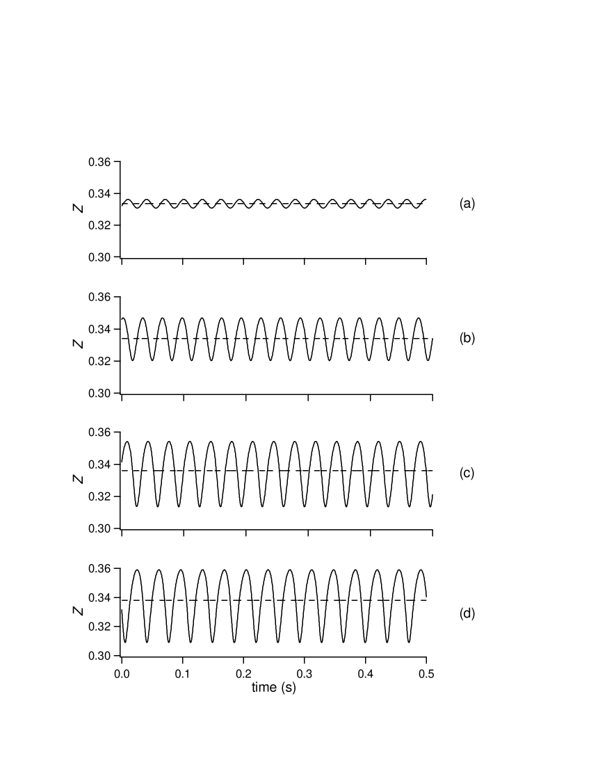
Figure 19: Time evolution of the atomic cloud location $Z$ in the close vicinity of the $\Delta_{1}$ bifurcation, on the unstable side. The dashed line represents the value of the unstable stationary solution $Z_{S}$. In (a), $\Delta_{0}=-0.4023$; in (b), $\Delta_{0}=-0.4020$; in (c), $\Delta_{0}=-0.4015$; in (d), $\Delta_{0}=-0.4010$. Other parameters are those of set #2 of Tab. 2.

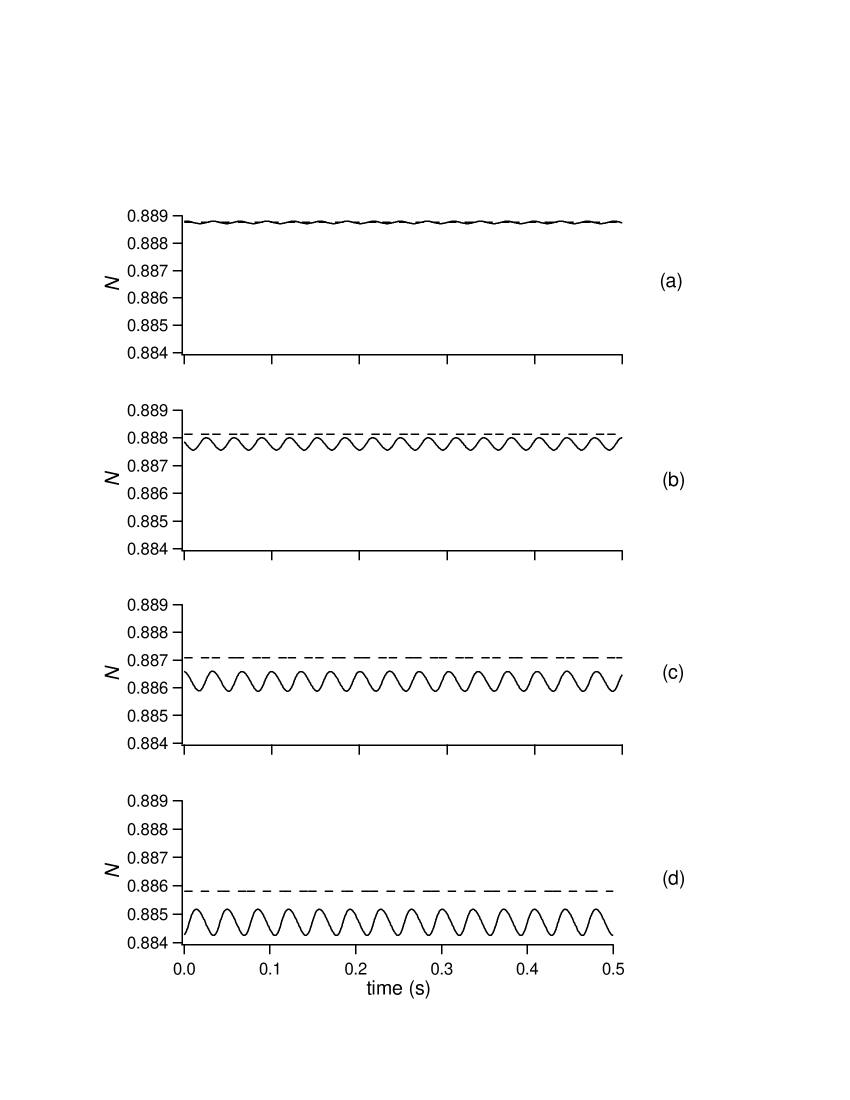
Figure 20: Time evolution of the atomic cloud population $N$ in the close vicinity of the $\Delta_{1}$ bifurcation, on the unstable side. The dashed line represents the value of the unstable stationary solution $N_{S}$. Parameters are the same as in Fig 19.

However, for $\Delta\geq\Delta_{1}^{\prime}$, the limit cycle becomes unstable and is replaced by another periodic orbit, with a much more complex shape (Fig. 21) and a much longer period. The amplitude is almost 5 times larger for $Z$ and more than 10 times for $N$. The trajectory consists in several different stages: a diverging spiral off the fixed point, followed by a large loop and a convergent spiral until the fixed point. The frequencies of the two oscillating stages are different: this is not surprising, as the diverging one is clearly linked to the fixed point, and thus to its eigenfrequency, contrary to the convergent one. One finds effectively a frequency of 24.4 Hz for the diverging spiral, corresponding exactly to the eigenfrequency ($\omega=2\pi\times 23.5\mathop{\rm Hz}$), while the frequency of the converging spiral is 77 Hz. However, the main frequency of the behavior is 2.6 Hz, i.e. one order of magnitude slower than that of the Hopf cycle. The properties of the trajectories, in particular the tangency to the unstable point and the large loop in the phase space, are characteristic from a homoclinic behavior, when the stable and unstable manifolds of the fixed point are almost connected. A accurate analysis of these manifolds would be necessary to conclude about this point. Note that in a very narrow interval around $\Delta_{1}^{\prime}$, generalized bistability occurs between the Hopf cycle and the homoclinic one.

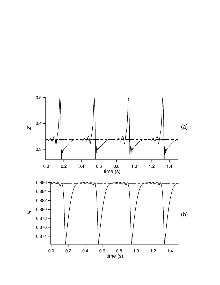
Figure 21: Time evolution of the atomic cloud location $Z$ in (a), and population $N$ in (b), for $\Delta_{0}=-0.4010$. Other parameters are the same as set #2 in Tab. 2.

When $\Delta_{0}$ is increased from $\Delta_{1}^{\prime}$, the cloud exhibits period doubling and chaos (Fig. 22). The trajectories keep the same shape, in particular with the two spiraling episodes and the large loop, but the periodicity is modified or is lost. For example, when the period is double, variations appear essentially on the amplitude of the loop together with that of the diverging oscillations (Fig. 22b). In the chaotic zone, the irregularities appear also on these amplitudes, but bursting events appear sometimes between these two stages (Fig. 22c). We did not perform a precise analysis of these behaviors, mainly because they appear on a so narrow interval that there is no chance to observe them experimentally. Indeed, chaos disappears for $\Delta>\Delta_{1}^{\prime\prime}$, with $\Delta_{1}^{\prime\prime}=-0.4005$, and thus the homoclinic behavior appears on an interval of $5\times 10^{-4}$. However, a simple test can be done by reconstructing the attractor of the dynamics (Fig. 23). A glance at the result shows a definite structure, and not random distributed points, and thus confirms that this behavior presents all the characteristics of deterministic chaos.

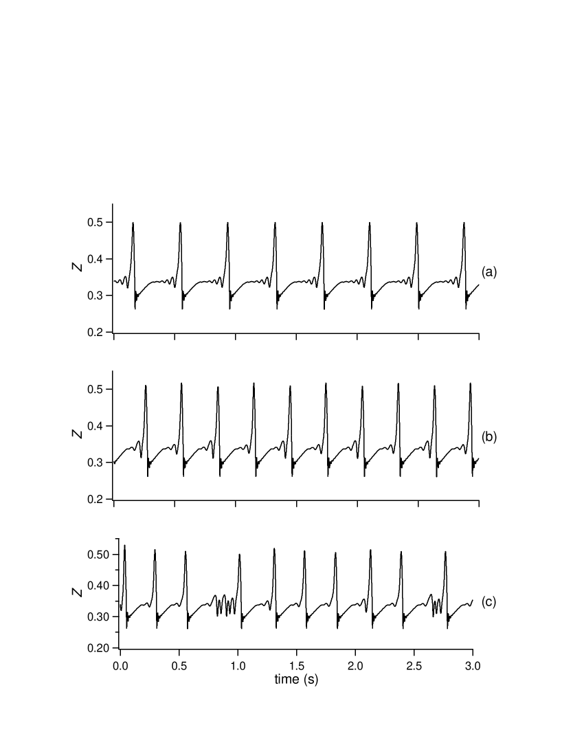
Figure 22: Time evolution of the atomic cloud location $Z$ in the vicinity of the chaotic zone. In (a), for $\Delta_{0}=-0.4010$, the motion is periodic; in (b), for $\Delta_{0}=-0.4006$, period doubling appears; in (c), for $\Delta_{0}=-0.4005$, the motion is chaotic. Other parameters are the same as set #2 in Tab. 2.

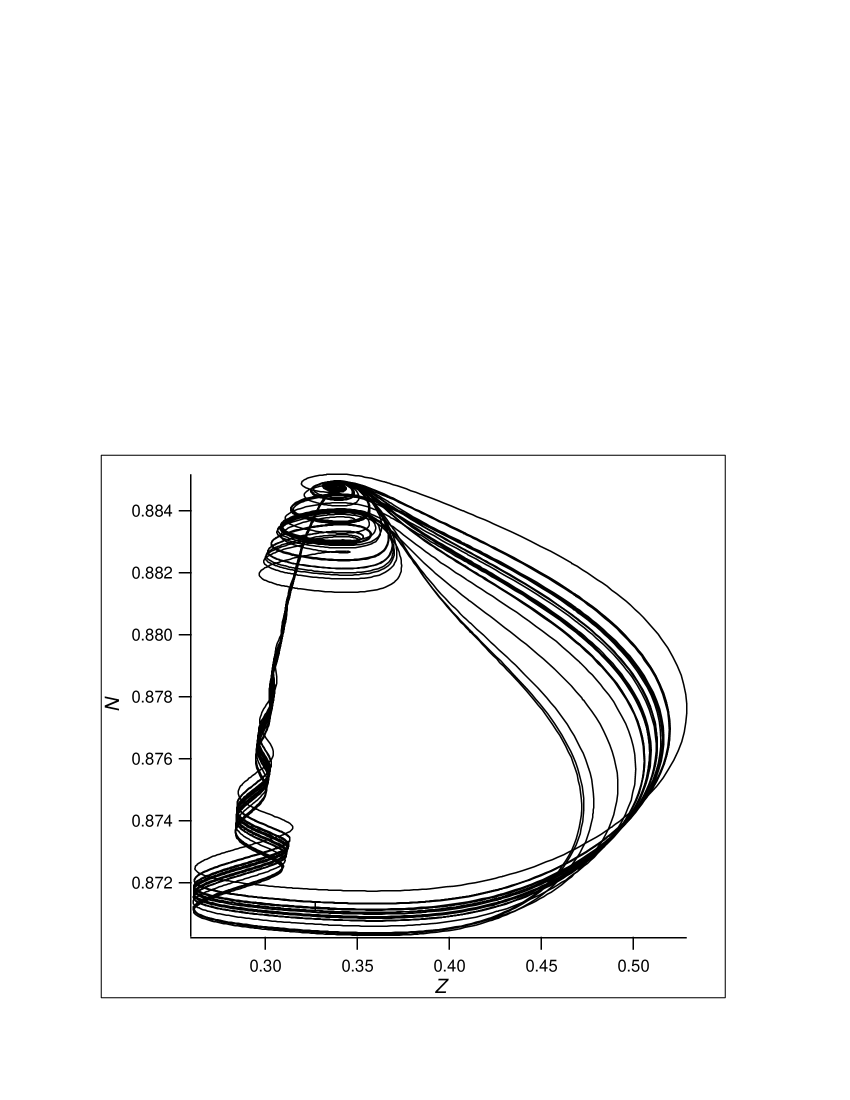
Figure 23: Chaotic trajectories of the cloud motion in the $(Z,N)$ phase space. $\Delta_{0}=-0.4005$. Other parameters are the same as in Tab. 2.

6.2 $C_{P}$ instabilities

For $\Delta_{0}>\Delta_{1}^{\prime\prime}$, the homoclinic behavior disappears, and a new type of periodic instabilities appear (Fig. 24). There is no fundamental difference between the homoclinic instabilities and the present behavior, except that the latter has a physical meaning, as it appears in the simulations on a significant $\Delta_{0}$ interval, about $0.04\Gamma$ for the present parameters. One observes in Fig. 24a the same three stages as in Fig. 22, which means that the origin of this behavior is the same as for the homoclinic instabilities. However, these three stages exist only in the close vicinity of $\Delta_{1}^{\prime\prime}$: when $\Delta_{0}$ is increased, the diverging helix around the fixed point disappears, and only the two stages independent from the fixed point remain (Fig. 24b and c). This means that in this new behavior, the trajectories never approach the fixed point, and thus the dynamics does not depend on the local properties of the fixed point.

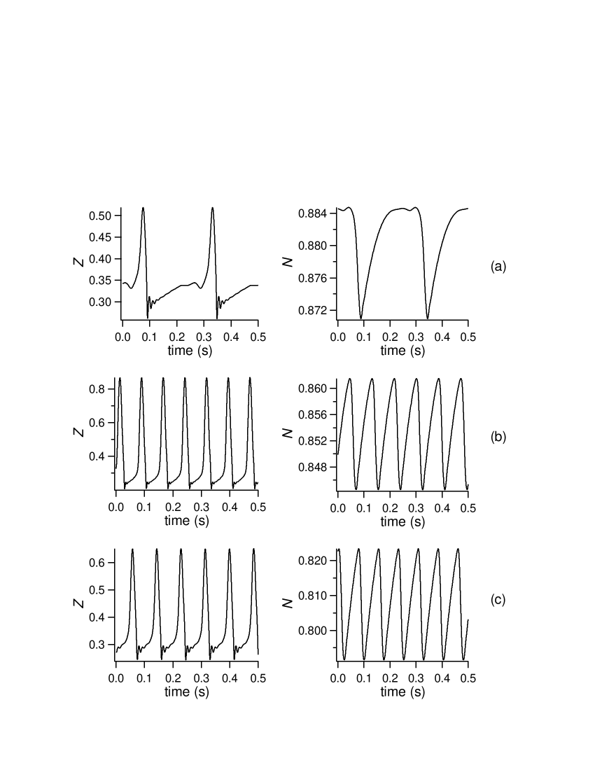
Figure 24: Time evolution of the atomic cloud location $Z$ (left) and population $N$ (right) in the unstable zone. In (a), $\Delta_{0}=-0.4004$; in (b), $\Delta_{0}=-0.39$; in (c), $\Delta_{0}=-0.37$. Other parameters are the same as in Tab. 2.

Each period of the new behavior may be divided in two stages with different durations. During the fast stage, $Z$ makes an oscillation, first growing then decreasing, while $N$ decreases; during the slow stage, $Z$ and $N$ grow. This is similar to that observed in experiments with C_P instabilities, and thus it is interesting to check if the other properties of C_P instabilities can be retrieve in the present dynamics.

Two untypical properties were noticed in the C_P instabilities, concerning the non zero amplitude of the oscillations when they appear, and their almost constant frequency along their interval of existence. The amplitude of the oscillations as a function of $\Delta_{0}$ is plotted in fig. 25. In $\Delta_{0}=-0.4$, when the instabilities appear, their amplitude is already almost 0.3. In fact, because the Hopf limit cycle exists on a very narrow interval, this is not strictly true. But from a physical point of view, it is clear that instabilities appear with a non zero amplitude, as in the experiments. Concerning the frequency, its value tends to zero in the vicinity of $\Delta_{1}^{\prime\prime}$, but it increases rapidly to reach a value of the order of 10 Hz, and remains between 10 Hz and 13 Hz on most of the unstable interval, as shown in Fig. 26 (the behavior for $\Delta_{0}>-0.36$ is discussed below). Finally, to complete the comparison with the experiments, Fig. 27 shows the power spectra of $Z$. In the vicinity of H₁, it is very characteristic, with a main frequency and large amplitude harmonics decreasing progressively (Fig. 27a), as in the experiments (Fig. 5). As the detuning is increased, the amplitude of the harmonics decreases, and several new frequencies appear in the spectrum, but each component has individually an amplitude negligible compared to the main frequency (Fig. 27b and c).

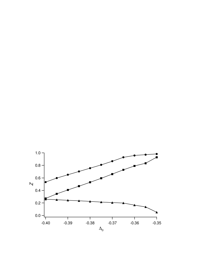
Figure 25: Amplitude of the dynamics versus detuning. The squares, discs and triangles corresponds respectively to the oscillation amplitude, the maximum value and the minimum value reached by $z$. Parameters are those of Tab. 2.

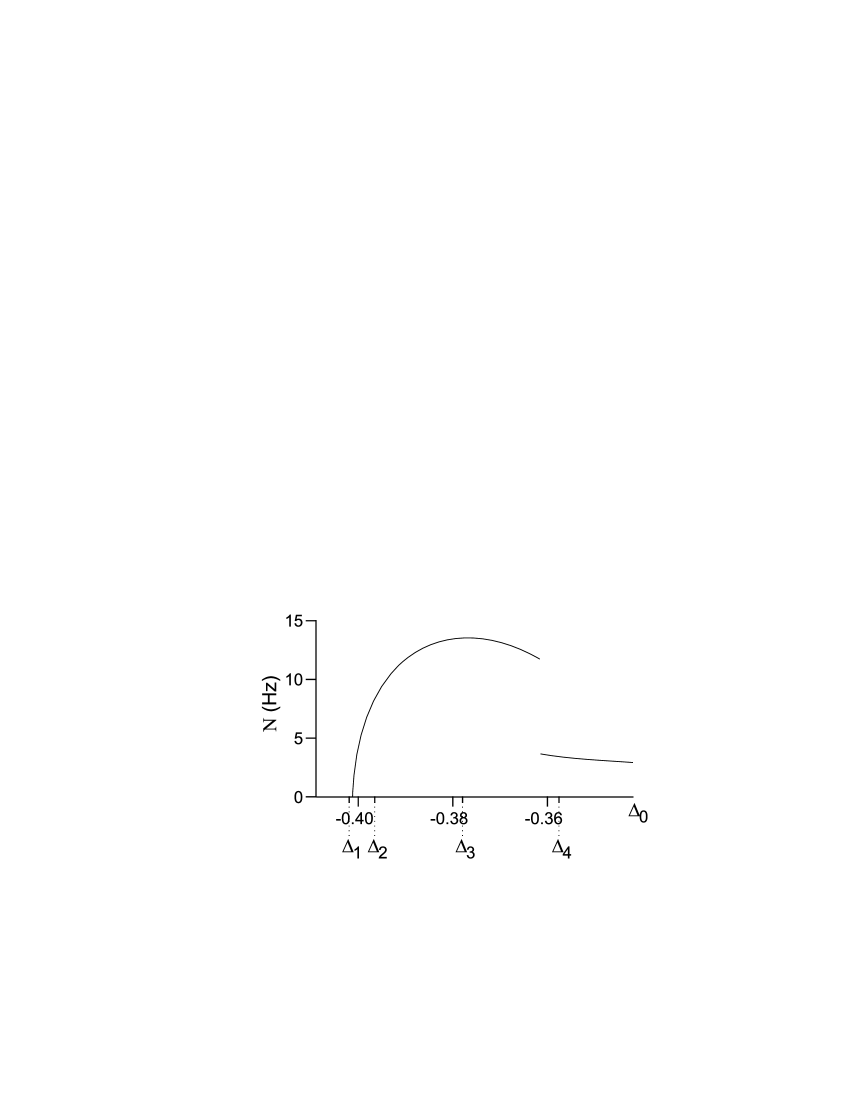
Figure 26: Evolution as a function of the detuning of the instabilities frequency.

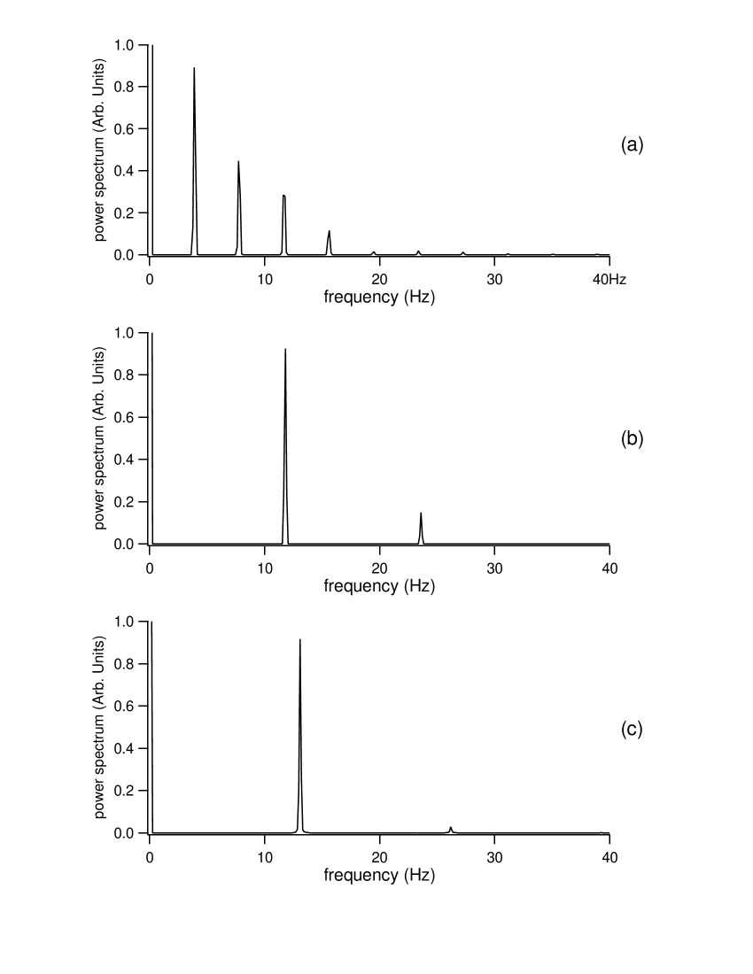
Figure 27: Power spectra of the atomic cloud location $Z$ in the unstable zone. Parameters are the same as in Fig.24.

To summarize, we found that the periodic instabilities in the vicinity of H₁ have the same shape, spectrum, amplitude evolution and frequency evolution as the C_P instabilities observed in the experiments; all these points confirm that the model reproduces here the C_P instabilities (Fig. 2 and 24).

However, several quantitative discrepancies appear between the present results and the experimental observations, as e.g. for the $\Delta_{0}$ values or the instabilities frequency. These differences are relatively small, except for the $\Delta_{0}$ interval where C_P instabilities exist: it is typically of the order of $1$ in the experiments, while it is smaller than $0.1$ in the simulations. This last value could be increased by increasing the value of $I_{1}$ in the simulations, reducing the difference to less than a factor 10. Considering the extreme simplicity of our model and its numerous approximations, it is clear that it is able to reproduce strikingly the C_P instabilities, with a surprisingly good agreement.

6.3 C₁ instabilities

In the experiments, C_P instabilities are replaced, as the detuning is changed, by C₁ instabilities. The difference between the two regimes appears mainly on the $n$ behavior, and in particular in the shape of the signal, which loses its regularity. The C₁ behavior is not observed in the present model. However, as discussed in the experimental section, the C₁ instabilities do not appear as a new deterministic regime, but rather as C_P instabilities slightly altered by noise. Thus, to test the ability of the present model to reproduce this behavior, it is necessary to add noise in the model. The results obtained in this case are discussed in the next section.

6.4 $C_{S}$ instabilities

Fig. 25 shows that the amplitude of the oscillations increases with $\Delta_{0}$, so that the maximum value explored by $z$ becomes larger and larger as $\Delta_{0}$ is increased. As a consequence, the maximum value reached by $z$ also increases, so that finally, the most distant atoms from the trap center, situated in $z+\Delta z/2$, where $\Delta z$ is the size of the cloud, reach the border of the trap, in $z_{0}$. In the model, these atoms are considered to be lost, and thus are subtracted to the total number of atoms in the trap. Therefore, a new process with a zero characteristic time appears in the model through this instantaneous decreasing of $n$. This new process leads to an immediate change of the dynamics frequency. This is illustrated in fig. 26, where the transition occurs in $\Delta_{0}=-0.361$. For these parameters, the frequency is divided by more than a factor 3, decreasing from 12 Hz to 3.7 Hz. The new dynamics is illustrated in Fig. 28. Although the global shape seems to be similar to the previous $C_{P}$ instabilities, a drastic difference appears on the dynamics of $N$, in particular concerning its oscillation amplitude. While the variations of $N$ as a function of time were small in the $C_{P}$ regime, they appear to be much larger in the present regime: in fig. 28a, $N$ varies on half of the total interval of values that it can take, and when $\Delta_{0}$ is still increased, this ratio reach 80%, with an oscillation from 0 to 0.8 (Fig. 28a). In the latter, the cloud empties completely every period, and then fill up progressively. This explain the large period of the regime, due to a longer time necessary to fill the cloud. This appears clearly when fig. 24 and fig. 28 are compared: the increasing of the period does not correspond to a global stretching of the dynamics, as the large oscillation of $Z$ remains on the same time scale, but rather is a consequence of the increasing of the interval between two oscillations.

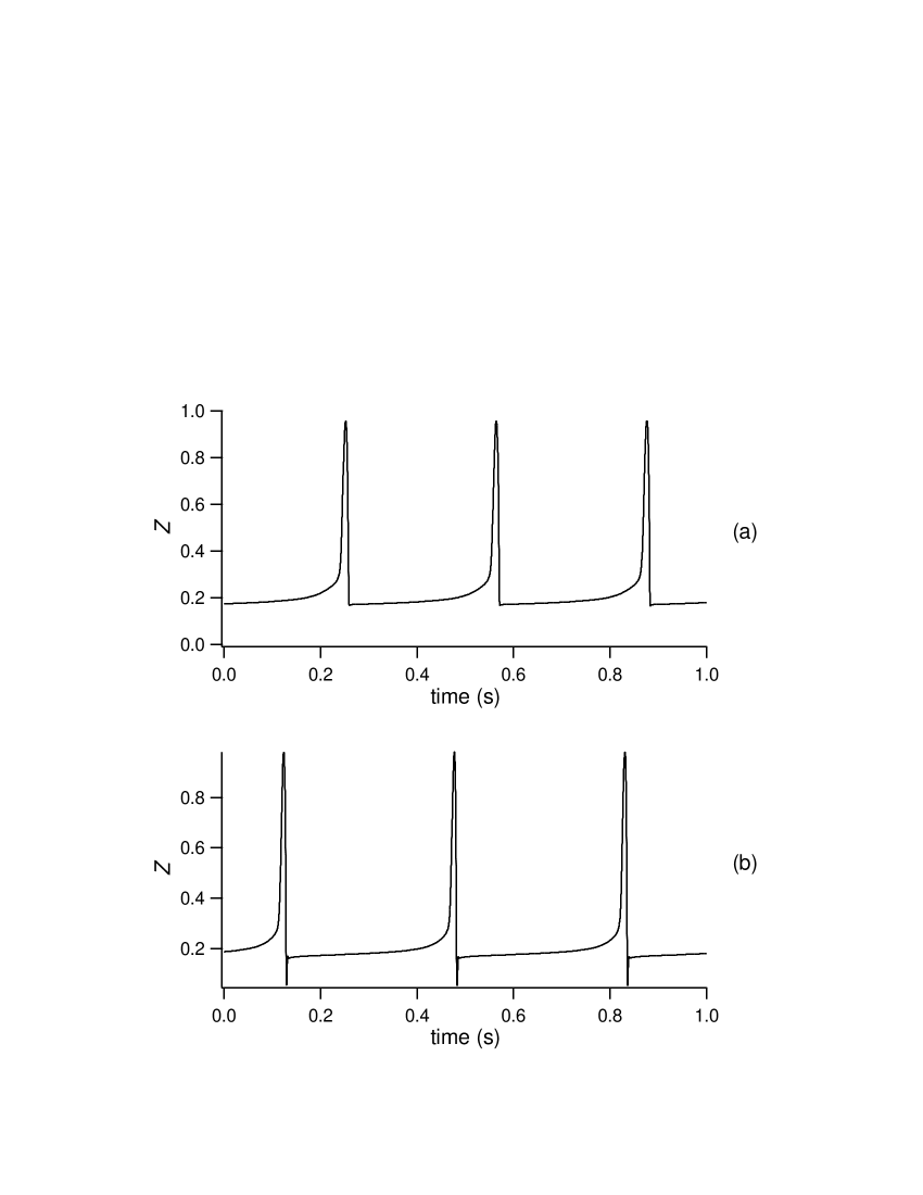
Figure 28: Time evolution of the atomic cloud location $Z$ (left) and population $N$ (right) in the unstable zone. In (a), $\Delta_{0}=-0.36$; in (b), $\Delta_{0}=-0.35$.

The spectrum confirms that the main frequency has decreased (Fig. 29). However, this is coupled with the appearance of large amplitude harmonics, decreasing slowly, so that components with higher frequency than in the $C_{P}$ regime keep a significant weight.

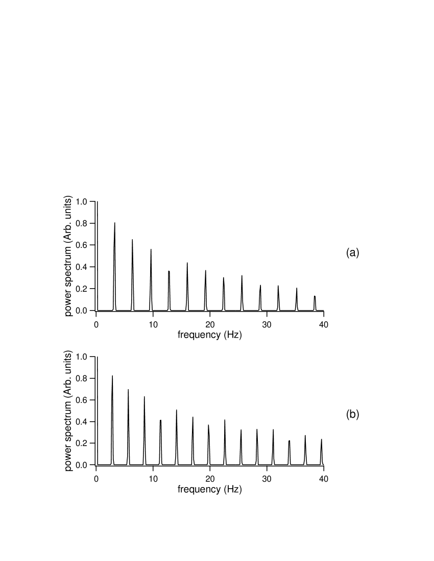
Figure 29: Power spectra of the atomic cloud location $Z$ in the unstable zone. Parameters are the same as in Fig.24.

This behavior has several common points with the $C_{S}$ instabilities described in the experimental section. In both cases, the regime is the continuation of the $C_{P}$ instabilities when the resonance is approached, the amplitude of the $z$ oscillation has a 100% contrast, that of $n$ are much larger than in $C_{P}$ regime, the shapes are similar, and new frequencies of higher value appear. But the regime obtained in the simulations remains periodic, contrary to that observed experimentally. However, as discussed in the experimental section, the origin of the erraticity observed in the experiments could be stochastic, rather than deterministic. Thus we can hope that the addition on noise in the model will transform the dynamics to reproduce the experimental results. This influence of noise on the dynamics is studied in the next section.

7 The effect of noise

Noise is known to be able to alter drastically the deterministic behavior of the MOT: in bruit2002 , it has been shown that a stationary behavior may be transformed, under the influence of noise, in a behavior similar to instabilities. Thus a complete study of the behaviors predicted by the present model must consider the possible alterations induced by noise on the dynamics. We present successively in this section the results obtained on C_P and C_S instabilities.

Fig. 30 illustrates the effect of noise on C_P instabilities, through the example of the regime plotted on Fig. 24c with 2% of noise on $I_{1}$. Although the behavior becomes less regular, with fluctuating amplitudes and a ruffling of the small secondary oscillations, the global behavior is unchanged, with a still rather regular period and the same global shape as without noise. Thus C_P instabilities appear to be robust against noise. However, if the response to noise is studied in more details, a slight increase of the noise influence appears when the C_S area is approached. This global behavior allows us to interprete both the C_P and the C₁ instabilities, which appear in fact to be the same dynamics, affected differently by noise: between $\Delta_{2}$ and $\Delta_{3}$, i.e. far from the C_S area, the C_P instabilities are very robust against noise, and the presence of technical noise in the experiment does not alter neither their shape nor their periodicity. As the C_S area is approached, the sensitivity of the C_P behavior to noise slightly increases, and, although the main characteristics of the C_P instabilities remain unchanged, the shape and periodicity of the regime are affected enough to give the feeling of a new regime, namely C₁ instabilities. Thus C₁ instabilities appear, as already suspected in the experimental section, as a C_P regime perturbed by noise

Figure 30: Time evolution of $Z$ for the same parameters as in Fig. 24c, but when noise is added on $I_{1}$. The noise level is 2%.

Fig. 31 shows how noise alters the dynamics of C_S instabilities. Although the amount of noise is the same as for C_P instabilities, it is clear that here, the dynamics is deeply transformed. Concerning the $Z$ dynamics, the shape of the oscillations remains almost unchanged, but the periodicity is drastically altered: indeed, the return time of the pulses varies randomly on a range larger than 100%. The explanation of these large fluctuations on the return time of the $Z$ pulses comes from the $N$ dynamics: here, the fluctuations appear on the amplitude of the variable. As the return time is connected to the reconstruction time of the cloud, it is logical that fluctuations in the initial population lead to fluctuations in the return time of $Z$. The strength of the effect is due, as for the stochastic dynamics described in bruit2002 , to an effect of amplification of noise, but through a different mechanism than that described in bruit2002 . Indeed, in the vicinity of $z_{0}$, noise modifies the state of the cloud just before the brutal decreasing of the population: it will be able to slow down the crossing of $z_{0}$, or on the contrary to quicken it. The consequence on the number of atoms lost in the process is immediate, leading to the large fluctuations of $N$ that can be seen in Fig. 31. If the resulting dynamics is compared with the experimental one illustrated in Fig. 4, the similarities between both dynamics appear clearly: the common points discussed in the previous section remain, and the discrepancies disappear. In particular, the fluctuations in the return time of the $z$ pulses, together with those in the amplitude of $n$, are now present: it is clear that we reproduce here the C_S instabilities.

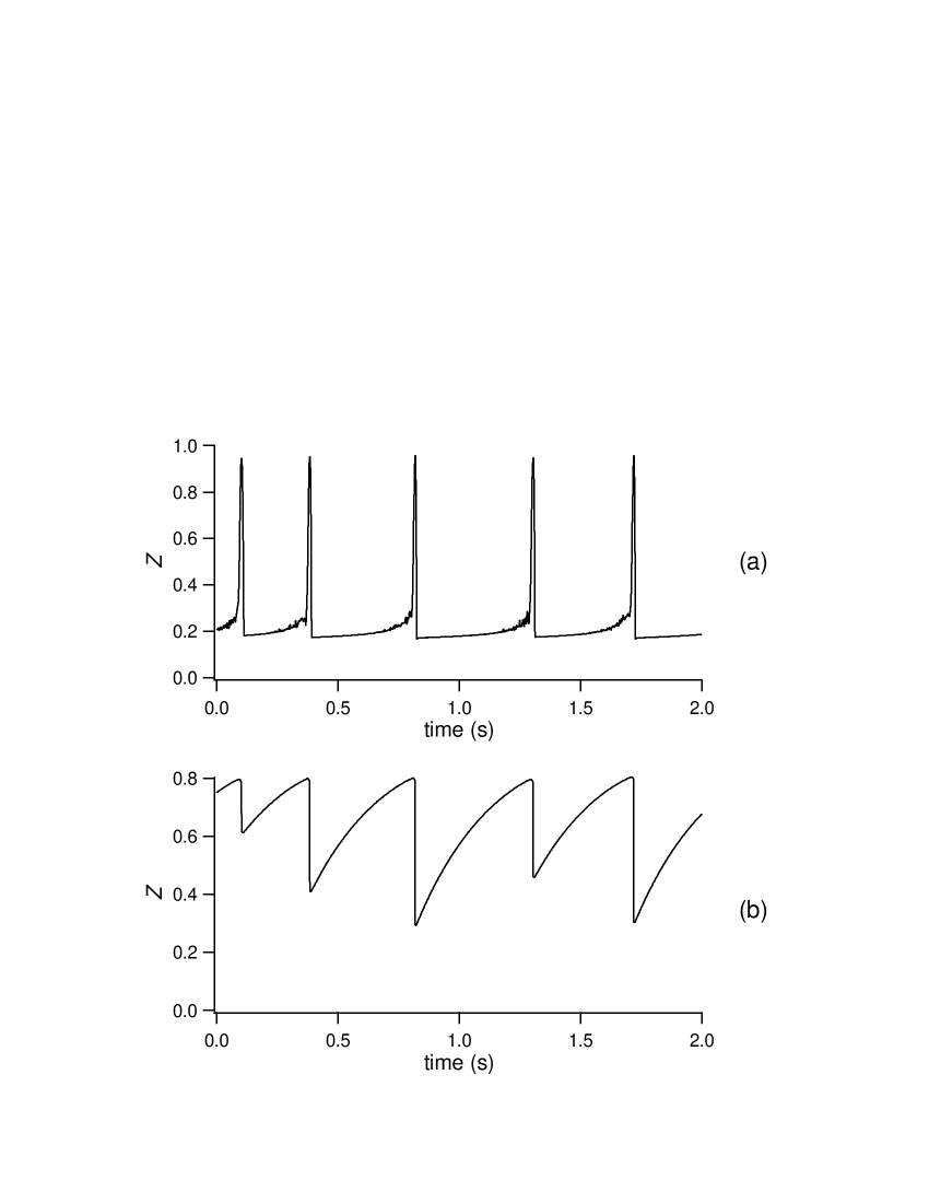
Figure 31: Time evolution of the (a) atomic cloud location and (b) population, for the same parameters as in Fig. 28, but when noise is added on $I_{1}$. The noise level is 2%.

This concludes the present study on the deterministic instabilities of the MOT, as we have been able to retrieve with our model all the behaviors observed experimentally. In particular, the dynamics that appeared as erratic is shown to be a deterministic periodic behavior perturbed by noise. This allows us to do the link with the studies reported in bruit2002 , as we show in this section that noise plays once again a key role in the dynamics of the MOT, although here the basis of the dynamics is deterministic.

8 Conclusion

The behavior of the cloud of cold atoms produced by a magneto-optical trap exhibits a rich variety of dynamics, that are well reproduce by a simple 1D model described by a set of three autonomous ordinary differential equations. In bruit2002 were described a set of noise-induced instabilities, linked to the topology of the stationary solutions. Here we show that experimentally, three different regimes of deterministic instabilities may also be observed, depending on the parameters of the MOT. Some of these regimes appear to be purely deterministic (C_P instabilities), some appear to be a mixture of deterministic instabilities and effects of noise (C₁ and C_S instabilities). Theoretically, the same model as in bruit2002 allows us to show that the existence of these deterministic instabilities are a direct consequence of the topological properties that induce for other parameters the stochastic instabilities studied in bruit2002 . This model shows that C₁ instabilities are just C_P instabilities perturbed by noise, while C_S instabilities are a nother deterministic regime appearing when the border of the trap beams are reached. This last regime is particularly sensitive to noise, and the resulting behavior appears as a deterministic instability highly perturbed by noise. Thus the present study confirms that noise plays a crucial role in the dynamics of the atomic cloud.

The present results have been obtained with a very simple model. Although the agreement with the experiments is surprisingly good, it is difficult to make qunatitative comparisons between such a 1D model and a 3D experiment. Therefore the next theoretical step would be to develop a 3D-model, where some of the parameters of the present model, as e.g. the cloud volume, become a function of the dynamics variables.

An interesting perspective of the present results is to study the possibility to take advantage of the existence of deterministic instabilities in the MOT. In particular, if a set of parameters could be found to widen enough the chaotic area, the techniques of control of chaos could be apply to reach various states that are not accessible otherwise, as e.g. denser or colder states. But even periodic behaviors can give new interesting informations about the MOT physics. Indeed, a complex dynamics covers a larger part of its phase space, and in return makes possible the determination of parameter values masked in stationary behaviors. More generally, a complex behavior enables the access to more information about its system, and appears usually as a good starting point for a better understanding of it.

9 Acknowledgments

The author thanks M. Fauquembergue for her participation in the elaboration of the model. The Laboratoire de Physique des Lasers, Atomes et Molécules is “Unité Mixte de Recherche de l’Université de Lille 1 et du CNRS” (UMR 8523). The Centre d’Etudes et de Recherches Lasers et Applications (CERLA) is supported by the Ministère chargé de la Recherche, the Région Nord-Pas de Calais and the Fonds Européen de Développement Economique des Régions.

References

- (1) S. Chu, Rev. Mod. Phys. 70, 685 (1998); C. Cohen-Tannoudji, Rev. Mod. Phys. 70, 707 (1998); W. Phillips, Rev. Mod. Phys. 70 (1998) 721
- (2) B. G. Klappauf, W. H. Oskay, D. A. Steck and M. G. Raizen, Physica D 131 (1999) 78
- (3) see, e.g., Y. Sortais, S. Bize, C. Nicolas, A. Clairon, C. Salomon and C. Williams 85 (2000) 3117, and references herein.
- (4) Gavin K. Brennen, Carlton M. Caves, Poul S. Jessen, and Ivan H. Deutsch, Phys. Rev. Lett. 82, (1999) 1060
- (5) L. Pitaevskii and S. Stringari, Phys. Rev. Lett. 87 (2001) 180402
- (6) D. Wilkowski, J. C. Garreau and D. Hennequin, Eur. Phys. J. D 2, (1998) 157
- (7) D. Wilkowski, J. Ringot, D. Hennequin and J. C. Garreau, Phys. Rev. Lett. 85, (2000) 1839
- (8) A. di Stefano, M. Fauquembergue, Ph. Verkerk and D. Hennequin, Phys. Rev. A 67 (2003) 033404
- (9) D. Hennequin, preprint physics/0304011, submitted to EPJD
- (10) see, e.g., Edward Ott, ”Chaos in Dynamical Systems”, Cambridge University Press, Cambridge (1993)
- (11) A. Zeni, J. A. C. Gallas, A. Fioretti, F. Papoff, B. Zambon and E. Arimondo, Phys. Lett. A 172 (1993) 247
- (12) T. Walker, D. Sesko and C. Wieman, Phys. Rev. Lett. 64, 408 (1990); D. W. Sesko, T. G. Walker and C. E. Wieman, J. Opt. Soc. Am. B 8, (1991) 946
- (13) J. Dalibard, Opt. Commun. 68, (1988) 203