Combined first–principles calculation and neural–network correction approach as a powerful tool in computational physics and chemistry

Abstract

Despite of their success, the results of first-principles quantum mechanical calculations contain inherent numerical errors caused by various approximations. We propose here a neural-network algorithm to greatly reduce these inherent errors. As a demonstration, this combined quantum mechanical calculation and neural-network correction approach is applied to the evaluation of standard heat of formation $\Delta\!_{\rm f}\!H^{\minuso}$ and standard Gibbs energy of formation $\Delta\!_{\rm f}\!G^{\minuso}$ for 180 organic molecules at 298 K. A dramatic reduction of numerical errors is clearly shown with systematic deviations being eliminated. For examples, the root–mean–square deviation of the calculated $\Delta\!_{\rm f}\!H^{\minuso}$ ($\Delta\!_{\rm f}\!G^{\minuso}$) for the 180 molecules is reduced from 21.4 (22.3) kcal$\cdotp$mol^-1 to 3.1 (3.3) kcal$\cdotp$mol^-1 for B3LYP/6-311+G(d,p) and from 12.0 (12.9) kcal$\cdotp$mol^-1 to 3.3 (3.4) kcal$\cdotp$mol^-1 for B3LYP/6-311+G(3df,2p) before and after the neural-network correction.

One of the Holy Grails of computational science is to quantitatively predict properties of matters prior to experiments. Despite the facts that the first-principles quantum mechanical calculation wtyang ; schaefer has become an indispensable research tool and experimentalists have been increasingly relying on computational results to interpret their experimental findings, the practically used numerical methods by far are often not accurate enough, in particular, for complex systems. This limitation is caused by the inherent approximations adopted in the first-principles methods. Because of computational cost, electron correlation has always been a difficult obstacle for first-principles calculations. Finite basis sets chosen in practical computations are not able to cover entire physical space and this inadequacy introduces further inherent computational errors. Effective core potential is frequently used to approximate the relativistic effects, resulting inevitably in errors for systems that contain heavy atoms. The accuracy of a density-functional theory (DFT) calculation is mainly determined by the exchange-correlation (XC) functional being employed wtyang , whose exact form is however unknown. Nevertheless, the results of first-principles quantum mechanical calculation can capture the essence of physics. For instance, the calculated results, despite that their absolute values may poorly agree with measurements, are usually of the same tendency among different molecules as their experimental counterpart. The quantitative discrepancy between the calculated and experimental results depends predominantly on the property of primary interest and, to a less extent, also on other related properties, of the material. There exists thus a sort of quantitative relation between the calculated and experimental results, as the aforementioned approximations, to a large extent, contribute to the systematic errors of specified first-principles methods. Can we develop general ways to eliminate the systematic computational errors and further to quantify the accuracies of numerical methods used? It has been proven an extremely difficult task to determine the calculation errors from the first-principles. Alternatives must be sought.

We propose here a neural–network algorithm to determine the quantitative relationship between the experimental data and the first-principles calculation results. The determined relation will subsequently be used to eliminate the systematic deviations of the calculated results, and thus, reduce the numerical uncertainties. Since its beginning in the late fifties, Neural Networks has been applied to various engineering problems, such as robotics, pattern recognition, speech, and etc. PRNN ; nature533 As the first application of Neural Networks to quantum mechanical calculations of molecules, we choose the standard heat of formation $\Delta\!_{\rm f}\!H^{\minuso}$ and standard Gibbs energy of formation $\Delta\!_{\rm f}\!G^{\minuso}$ at 298.15 K as the properties of interest.

A total of 180 small- or medium-sized organic molecules, whose $\Delta\!_{\rm f}\!H^{\minuso}$ and $\Delta\!_{\rm f}\!G^{\minuso}$ values are well documented in Refs. McGraw, ; crchandbook, ; thermodata, , are selected to test our proposed approach. The tabulated values of $\Delta\!_{\rm f}\!H^{\minuso}$ and $\Delta\!_{\rm f}\!G^{\minuso}$ in the three references differ less than 1.0 kcal$\cdotp$mol^-1 for same molecule. The uncertainties of all $\Delta\!_{\rm f}\!H^{\minuso}$ values are less than 1.0 kcal$\cdotp$mol^-1, while those of $\Delta\!_{\rm f}\!G^{\minuso}$s are not reported in Refs. McGraw, ; crchandbook, ; thermodata, . These selected molecules contain elements such as H, C, N, O, F, Si, S, Cl and Br. The heaviest molecule contains 14 heavy atoms, and the largest has 32 atoms. We divide these molecules randomly into the training set (150 molecules) and the testing set (30 molecules). The geometries of 180 molecules are optimized via B3LYP/6-311+G(d,p) g98 calculations and the zero point energies (ZPEs) are calculated at the same level. The enthalpy and Gibbs energy of each molecule are calculated at both B3LYP/6-311+G(d,p) and B3LYP/6-311+G(3df,2p). g98 B3LYP/6-311+G(3df,2p) employs a larger basis set than B3LYP/6-311+G(d,p). The unscaled B3LYP/6-311+G(d,p) ZPE is employed in the $\Delta\!_{\rm f}\!H^{\minuso}$ and $\Delta\!_{\rm f}\!G^{\minuso}$ calculations. The strategies in reference jcp97g2, are adopted to calculate $\Delta\!_{\rm f}\!H^{\minuso}$ and $\Delta\!_{\rm f}\!G^{\minuso}$. The calculated $\Delta\!_{\rm f}\!H^{\minuso}$ and $\Delta\!_{\rm f}\!G^{\minuso}$ for B3LYP/6-311+G(d,p) and B3LYP/6-311+G(3df,2p) are compared to their experimental counterparts in Figs. 1 and  2, respectively. The horizontal coordinates are the raw calculated data, and the vertical coordinates are the experimental values. The dashed lines are where the vertical and horizontal coordinates are equal, i.e., where the B3LYP calculations and experiments would have the perfect match. The raw calculation values are mostly below the dashed line, i.e., most raw $\Delta\!_{\rm f}\!H^{\minuso}$ and $\Delta\!_{\rm f}\!G^{\minuso}$ are larger than the experimental data. In another word, there are systematic deviations for both B3LYP $\Delta\!_{\rm f}\!H^{\minuso}$ and $\Delta\!_{\rm f}\!G^{\minuso}$. Compared to the experimental measurements, the root–mean–square (RMS) deviations for $\Delta\!_{\rm f}\!H^{\minuso}$ ($\Delta\!_{\rm f}\!G^{\minuso}$) are 21.4 (22.3) and 12.0 (12.9) kcal$\cdotp$mol^-1 for B3LYP/6-311+G(d,p) and B3LYP/6-311+G(3df,2p) calculations, respectively. In Table 1 we compare the B3LYP and experimental $\Delta\!_{\rm f}\!H^{\minuso}$s for 10 of 180 molecules. Overall, B3LYP/6-311+G(3df,2p) calculations yield better agreements with the experiments than B3LYP/6-311+G(d,p). In particular, for small molecules with few heavy elements B3LYP/6-311+G(3df,2p) calculations result in very small deviations from the experiments. For instance, the $\Delta\!_{\rm f}\!H^{\minuso}$ deviations for CH₄ and CS₂ are only -0.5 and 0.6 kcal$\cdot$mol^-1, respectively. Our B3LYP/6-311+G(3df,2p) calculation results are also in good agreements with those of reference jcp97g2, which employed a similar calculation strategy except that their ZPEs were scaled by a factor of 0.98 or 0.96 and their geometries were optimized at B3LYP/6-31+G(d). For large molecules, both B3LYP/6-311+G(d,p) and B3LYP/6-311+G(3df,2p) calculations yield quite large deviations from their experimental counterparts.

Table 1: Experimental and calculated $\Delta\!_{\rm f}\!H^{\minuso}$(298 K) for ten selected compounds (all data are in the units of kcal$\cdot$mol^-1)

		Deviations (Theory-Expt.)
Molecules	Expt.	DFT1	DFT1-NN	DFT2	DFT2-NN	DFT3
CF2O	-152.9$\pm{0.4}$	20.0	6.9	8.7	6.8	9.1
CH2Cl2	-22.8$\pm{0.3}$	10.6	3.6	5.0	4.9	4.6
CH2F2	-108.1$\pm{0.2}$	8.0	0.9	0.6	0.6	0.0
CH4	-17.8$\pm{0.1}$	1.1	1.1	-0.5	1.0	-1.6
CS2	27.9$\pm{0.2}$	8.7	3.3	0.6	3.2	0.2
C5H12	-35.1$\pm{0.2}$	16.7	-2.1	9.9	-2.2	–
C5H12O	-75.3$\pm{0.3}$	23.2	0.2	14.0	0.1	–
C6H14	-41.1 $\pm{0.2}$	25.1	1.4	17.0	1.5	–
C8H10	4.6 $\pm{0.3}$	25.7	0.5	13.3	1.0	–
C9H12	-2.3 $\pm{0.3}$	31.3	0.9	17.6	1.8	–

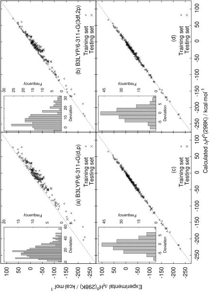
Figure 1: Experimental $\Delta\!_{\rm f}\!H^{\minuso}$ versus calculated $\Delta\!_{\rm f}\!H^{\minuso}$ for all 180 compounds. (a) and (b) are for raw B3LYP/6-311+G(d,p) and B3LYP/6-311+G(3df,2p) results, respectively. (c) and (d) are for neural-network corrected B3LYP/6-311+G(d,p) and B3LYP/6-311+G(3df,2p) $\Delta\!_{\rm f}\!H^{\minuso}$s, respectively. In (c) and (d), triangles are for the training set and crosses for the testing set. Inserts are the histograms for the differences between the experimental and calculated $\Delta\!_{\rm f}\!H^{\minuso}$s. All values are in the units of kcal$\cdot$mol^-1.

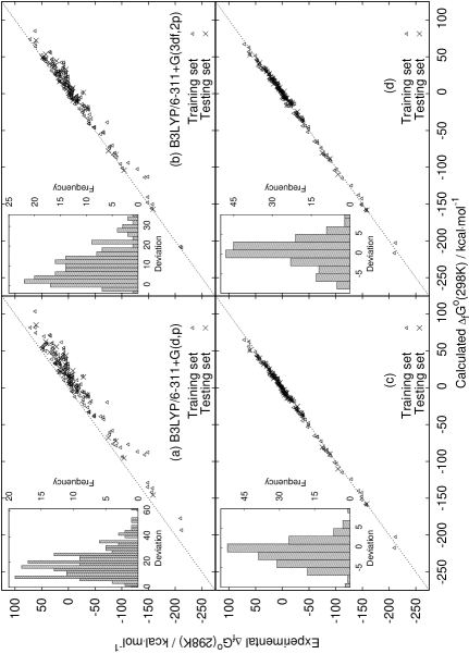
Figure 2: Experimental $\Delta\!_{\rm f}\!G^{\minuso}$ versus calculated $\Delta\!_{\rm f}\!G^{\minuso}$ for all 180 compounds. (a) and (b) are for raw B3LYP/6-311+G(d,p) and B3LYP/6-311+G(3df,2p) results, respectively. (c) and (d) are for neural-network corrected B3LYP/6-311+G(d,p) and B3LYP/6-311+G(3df,2p) $\Delta\!_{\rm f}\!G^{\minuso}$s, respectively. Legends, units and inserts are similar to those of Fig. 1.

Our neural network adopts a three-layer architecture which has an input layer consisted of input from the physical descriptors and a bias, a hidden layer containing a number of hidden neurons, and an output layer that outputs the corrected values for $\Delta\!_{\rm f}\!H^{\minuso}$ or $\Delta\!_{\rm f}\!G^{\minuso}$ (see Fig. 3). The number of hidden neurons is to be determined. The most important issue is to select the proper physical descriptors of our molecules, which are to be used as the input for our neural network. The calculated $\Delta\!_{\rm f}\!H^{\minuso}$ and $\Delta\!_{\rm f}\!G^{\minuso}$ contain the essence of exact $\Delta\!_{\rm f}\!H^{\minuso}$ and $\Delta\!_{\rm f}\!G^{\minuso}$, respectively, and are thus obvious choices of the primary descriptor for correcting $\Delta\!_{\rm f}\!H^{\minuso}$ and $\Delta\!_{\rm f}\!G^{\minuso}$, respectively. We observe that the size of a molecule affects the accuracies of calculations. The more atoms a molecule has, the worse the calculated $\Delta\!_{\rm f}\!H^{\minuso}$ and $\Delta\!_{\rm f}\!G^{\minuso}$ are. This is consistent with the general observations in the field. jcp97g2 The total number of atoms $N_{t}$ in a molecule is thus chosen as the second descriptor for the molecule. ZPE is an important parameter in calculating $\Delta\!_{\rm f}\!H^{\minuso}$ and $\Delta\!_{\rm f}\!G^{\minuso}$. Its calculated value is often scaled in evaluating $\Delta\!_{\rm f}\!H^{\minuso}$ and $\Delta\!_{\rm f}\!G^{\minuso}$, jcp97g2 and it is thus taken as the third physical descriptor. Finally, the number of double bonds, $N_{db}$, is selected as the fourth and last descriptor to reflect the chemical structure of the molecule.

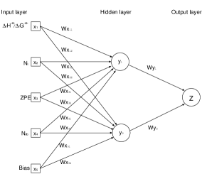
Figure 3: Structure of our neural network.

To ensure the quality of our neural network, a cross-validation procedure is employed to determine our neural network. rbfnn We divide further randomly 150 training molecules into five subsets of equal size. Four of them are used to train the neural network, and the fifth to validate its predictions. This procedure is repeated 5 times in rotation. The number of neurons in the hidden layer is varied from 2 to 10 to decide the optimal structure of our neural network. We find that the hidden layer containing two neurons yields best overall results. Therefore, the 5-2-1 structure is adopted for our neural network as depicted in Fig. 3. The input values at the input layer, $x_{1}$, $x_{2}$, $x_{3}$, $x_{4}$ and $x_{5}$, are scaled $\Delta\!_{\rm f}\!H^{\minuso}$ (or $\Delta\!_{\rm f}\!G^{\minuso}$), $N_{t}$, ZPE, $N_{db}$ and bias, respectively. The bias $x_{5}$ is set to 1. The weights $\{Wx_{ij}\}$s connect the input layer $\{x_{i}\}$ and the hidden neurons $y_{1}$ and $y_{2}$, and $\{Wy_{j}\}$s connect the hidden neurons and the output Z which is the scaled $\Delta\!_{\rm f}\!H^{\minuso}$ or $\Delta\!_{\rm f}\!G^{\minuso}$ upon neural-network correction. The output Z is related to the input $\{x_{i}\}$ as

$$Z=\sum_{j=1,2}Wy_{j}~{}Sig(\sum_{i=1,5}Wx_{ij}~{}x_{i}),$$ (1)

where $Sig(v)={1\over 1+exp(-\alpha v)}$ and $\alpha$ is a parameter that controls the switch steepness of Sigmoidal function $Sig(v)$. An error back-propagation learning procedure nature533 is used to optimize the values of $Wx_{ij}$ and $Wy_{j}$($i=1,2,3,4,5$ and $j=1,2$). In Figs. 1c, 1d, 2c and 2d, the triangles belong to the training set and the crosses to the testing set. Compared to the raw calculated results, the neural-network corrected values are much closer to the experimental values for both training and testing sets. More importantly, the systematic deviations for $\Delta\!_{\rm f}\!H^{\minuso}$ and $\Delta\!_{\rm f}\!G^{\minuso}$ in Figs. 1a, 1b, 2a and 2b are eliminated, and the resulting numerical deviations are reduced substantially. This can be further demonstrated by the error analysis performed for the raw and neural-network corrected $\Delta\!_{\rm f}\!H^{\minuso}$s and $\Delta\!_{\rm f}\!G^{\minuso}$s of all 180 molecules. In the inserts of Figs. 1 and 2, we plot the histograms for the deviations (from the experiments) of the raw B3LYP $\Delta\!_{\rm f}\!H^{\minuso}$s and $\Delta\!_{\rm f}\!G^{\minuso}$s and their neural–network corrected values. Obviously, the raw calculated $\Delta\!_{\rm f}\!H^{\minuso}$s and $\Delta\!_{\rm f}\!G^{\minuso}$s have large systematic deviations while the neural–network corrected $\Delta\!_{\rm f}\!H^{\minuso}$s and $\Delta\!_{\rm f}\!G^{\minuso}$s have virtually no systematic deviations. Moreover, the remaining numerical deviations are much smaller. Upon the neural-network corrections, the RMS deviations of $\Delta\!_{\rm f}\!H^{\minuso}$s ($\Delta\!_{\rm f}\!G^{\minuso}$s) are reduced from 21.4 (22.3) kcal$\cdot$mol^-1 to 3.1 (3.3) kcal$\cdot$mol^-1 and 12.0 (12.9) kcal$\cdot$mol^-1 to 3.3 (3.4) kcal$\cdot$mol^-1 for B3LYP/6-311+G(d,p) and B3LYP/6-311+G(3df,2p), respectively. Note that the error distributions after the neural–network correction are of approximate Gaussian distributions (see Figs. 2c and  2d). Although the raw B3LYP/6-311+G(d,p) results have much larger deviations than those of B3LYP/6-311+G(3df, 2p), the neural–network corrected values of both calculations have deviations of the same magnitude. This implies that it is sufficient to employ the smaller basis set 6-311+G(d,p) in our combined DFT calculation and neural–network correction (or DFT-NEURON) approach. The neural–network algorithm can correct easily the deficiency of a small basis set. Therefore, the DFT-NEURON approach can potentially be applied to much larger systems. In Table 1 we also list the neural–network corrected $\Delta\!_{\rm f}\!H^{\minuso}$s of the 10 molecules. The deviations of large molecules are of the same magnitude as those of small molecules. Unlike other quantum mechanical calculations that usually yield worse results for larger molecules than for small ones, the DFT-NEURON approach does not discriminate against the large molecules.

Analysis of our neural network reveals that the weights connecting the input for $\Delta\!_{\rm f}\!H^{\minuso}$ or $\Delta\!_{\rm f}\!G^{\minuso}$ have the dominant contribution in all cases. This confirms our fundamental assumption that the calculated $\Delta\!_{\rm f}\!H^{\minuso}$ ($\Delta\!_{\rm f}\!G^{\minuso}$) captures the essential values of exact $\Delta\!_{\rm f}\!H^{\minuso}$ ($\Delta\!_{\rm f}\!G^{\minuso}$). The input for the second physical descriptor, $N_{t}$, has quite large weights in all cases. In particular, when the smaller basis set 6-311+G(d,p) is adopted in the B3LYP calculations, $N_{t}$ has the second largest weights. It is found that the raw $\Delta\!_{\rm f}\!H^{\minuso}$ and $\Delta\!_{\rm f}\!G^{\minuso}$ deviations are roughly proportional to $N_{t}$, which confirms the importance of $N_{t}$ as a significant descriptor of our neural network. The bias contributes to the correction of systematic deviations in the raw calculated data, and has thus significant weights. When the larger basis set 6-311+G(3df,2p) is used, the bias has the second largest weights for all cases. ZPE has been often scaled to account for the discrepancies of $\Delta\!_{\rm f}\!H^{\minuso}$s or $\Delta\!_{\rm f}\!G^{\minuso}$s between calculations and experiments, jcp97g2 and it is thus expected to have large weights. This is indeed the case, especially when the smaller basis set 6-311+G(d,p) is adopted in calculations. In all cases the number of double bonds, $N_{db}$, has the smallest but non-negligible weights. In Table 2 we list the values of $\{Wx_{ij}\}$ and $\{Wy_{j}\}$ of the two neural networks for correcting $\Delta\!_{\rm f}\!G^{\minuso}$s of B3LYP/6-311+G(d,p) and B3LYP/6-311+G(3df,2p) calculations.

Table 2: Weights of DFT-Neural Networks for $\Delta\!_{\rm f}\!G^{\minuso}$

				DFT1-NN									DFT2-NN
Weights				y1				y2					y1				y2
Wx1j				0.78				-0.72					0.83				-0.73
Wx2j				-0.60				0.02					-0.30				0.02
Wx3j				0.44				0.02					0.18				0.02
Wx4j				0.07				0.24					0.05				0.17
Wx5j				-0.42				-0.04					-0.46				0.01
Wyj				1.48				-0.57					1.44				-0.47

Our DFT-NEURON approach has a RMS deviation of $\sim$3 kcal$\cdot$mol^-1 for the 180 small- to medium-sized organic molecules. This is slightly larger than their experimental uncertainties. McGraw ; crchandbook ; thermodata The physical descriptors adopted in our neural network, the raw calculated $\Delta\!_{\rm f}\!H^{\minuso}$ or $\Delta\!_{\rm f}\!G^{\minuso}$, the number of atoms $N_{t}$, the number of double bonds $N_{db}$ and the ZPE are quite general, and are not limited to special properties of organic molecules. The DFT-NEURON approach developed here is expected to yield a RMS deviation of $\sim$3 kcal$\cdot$mol^-1 for $\Delta\!_{\rm f}\!H^{\minuso}$s and $\Delta\!_{\rm f}\!G^{\minuso}$s of any small- to medium-sized organic molecules. G2 method jcp97g2 results are more accurate for small molecules. However, our approach is much more efficient and can be applied to much larger systems. To improve the accuracy of the DFT-NEURON approach, we need more and better experimental data, and possibly, more and better physical descriptors for the molecules. Besides $\Delta\!_{\rm f}\!H^{\minuso}$ and $\Delta\!_{\rm f}\!G^{\minuso}$, the DFT-NEURON approach can be generalized to calculate other properties such as ionization energy, dissociation energy, absorption frequency, band gap and etc. The raw first-principles calculation property of interest contains its essential value, and is thus always the primary descriptor. Since the raw calculation error accumulates as the molecular size increases, the number of atoms $N_{t}$ should thus be selected as a descriptor for any DFT-NEURON calculations. Additional physical descriptors should be chosen according to their relations to the property of interest and to the physical and chemical structures of the compounds. Others have used Neural Networks to determine the quantitative relationship between the experimental thermodynamic properties and the structure parameters of the molecules. rbfnn We distinct our work from others by utilizing specifically the first-principles methods and with the objective to improve quantum mechanical results. Since the first-principles calculations capture readily the essences of the properties of interest, our approach is more reliable and covers much a wider range of molecules or compounds.

To summarize, we have developed a promising new approach to improve the results of first-principles quantum mechanical calculations and to calibrate their uncertainties. The accuracy of DFT-NEURON approach can be systematically improved as more and better experimental data are available. As the systematic deviations caused by small basis sets and less sophisticated methods adopted in the calculations can be easily corrected by Neural Networks, the requirements on first-principles calculations are modest. Our approach is thus highly efficient compared to much more sophisticated first-principles methods of similar accuracy, and more importantly, is expected to be applied to much larger systems. The combined first-principles calculation and neural-network correction approach developed in this work is potentially a powerful tool in computational physics and chemistry, and may open the possibility for first-principles methods to be employed practically as predictive tools in materials research and design.

We thank Prof. YiJing Yan for extensive discussion on the subject and generous help in manuscript preparation. Support from the Hong Kong Research Grant Council (RGC) and the Committee for Research and Conference Grants (CRCG) of the University of Hong Kong is gratefully acknowledged.

References

- (1)
- (2) R. G. Parr and W. Yang, Density-Functional Theory of Atoms and Molecules (Oxford University Press, New York, 1989), and references therein.
- (3) H. F. Schaefer III, Methods of electronic structure theory (Plenum press, New York and London, 1977), and references therein.
- (4) B. D. Ripley, Pattern recognition and neural networks, (New York : Cambridge University Press, 1996).
- (5) D. E. Rumelhart, G. E. Hinton, R. J. Williams, Nature, , 533(1986).
- (6) C. L. Yaws, Chemical properties Handbook (McGraw-Hill, New York, 1999).
- (7) D. R. Lide, CRC Handbook of Chemistry and Physics 3rd Electronic ed (CRC Press, Boca Raton, FL 2000).
- (8) J. B. Pedley, R. D. Naylor, and S. P. Kirby, Thermochemical data of organic compounds 2nd ed (Chapman and Hall, New York, 1986).
- (9) M. J. Frisch et al. Gaussian 98, Revision A.11.3 Gaussian, Inc., Pittsburgh PA, 2002.
- (10) L. A. Curtiss, K. Raghavachari, P. C. Redfern, J. A. Pople, J. Chem. Phys., 106, 1063 (1997).
- (11) X. Yao, X. Zhang, R. Zhang, M. Liu, Z. Hu, B. Fan, Computers & Chemistry, 25, 475 (2001).