Entropy and information in neural spike trains: Progress on the sampling problem

Abstract

The major problem in information theoretic analysis of neural responses and other biological data is the reliable estimation of entropy–like quantities from small samples. We apply a recently introduced Bayesian entropy estimator to synthetic data inspired by experiments, and to real experimental spike trains. The estimator performs admirably even very deep in the undersampled regime, where other techniques fail. This opens new possibilities for the information theoretic analysis of experiments, and may be of general interest as an example of learning from limited data.

I Introduction

There has been considerable progress in using information theoretic methods to sharpen and to answer many questions about the structure of the neural code Bialek et al. (1991); Theunissen and Miller (1991); Berry et al. (1997); Strong et al. (1998); Borst and Theunissen (1999); Brenner et al. (2000a); Reinagel and Reid (2000); Reich et al. (2001). Where classical experimental approaches have focused on mean response of neurons to relatively simple stimuli, information theoretic methods have the power to quantify the responses to arbitrarily complex and even fully natural stimuli Rieke et al. (1997); Lewen et al. (2001), taking account of both the mean response and its variability in a rigorous way, independent of detailed modeling assumptions. Measurements of entropy and information in spike trains also allow us to test directly the hypothesis that the neural code adapts to the distribution of sensory inputs, optimizing the rate or efficiency of information transmission Barlow (1959, 1961); Laughlin (1981); Brenner et al. (2000b); Fairhall et al. (2001).

A problem with such measurements is that entropy and information depend explicitly on the full distribution of neural responses, just a limited sample of which is provided by experiments. In particular, we need to know the distribution of responses to each stimulus in our ensemble, and the number of samples from this distribution is limited by the number of times the full set of stimuli can be repeated. For natural stimuli with long correlation times the time required to present a useful “full set of stimuli” is long, limiting the number of independent samples we can obtain from stable neural recordings. Furthermore, natural stimuli generate neural responses of high timing precision, and thus the space of meaningful responses itself is very large Mainen and Sejnowski (1995); de Ruyter van Steveninck et al. (1997); Berry et al. (1997); Lewen et al. (2001). These factors make the sampling problem more serious as we move to more interesting and natural stimuli.

A natural response to this problem is to give up the generality of a completely model independent information theoretic approach. Some explicit help from models is required to regularize learning of the underlying probability distributions from the experiments. The question is if we can keep the generality of our analysis by introducing the gentlest of regularizations for the abstract learning problem, or if we need stronger assumptions about the structure of the neural code itself (for example, introducing a metric on the space of responses Victor and Purpura (1997); Victor (2002)).

A classical problem suggests that we may succeed even with very weak assumptions. Remember that one needs to have only $N\sim 23$ people in a room before any two of them are reasonably likely to share the same birthday. This is much less than $K=365$, the number of possible birthdays. Turning this around, we can estimate the number of possible birthdays by polling $N$ people and counting how often we find coincidences. Once $N$ is large enough to have observed a few of those, we can get a pretty good estimate of $K$. This will happen with a significant probability for $N\sim\sqrt{K}\ll K$.

The idea of estimating entropy by counting coincidences was proposed long ago by Ma Ma (1981) for physical systems in the microcanonical ensemble where distributions should be uniform at fixed energy. Clearly, if we could generalize the Ma idea to arbitrary distributions, then we would be able to explore a much wider variety of question about information in the neural code. Here we argue that a simple and abstract Bayesian prior, introduced in Ref. Nemenman et al. (2002), comes close to the objective.

It is well known that, for $N<K$, there are no universally good entropy estimators Paninski (2003); Batu et al. (2002). Thus the main question is: does a particular method work well only for (possibly irrelevant) abstract model problems, or can it also be trusted for natural data? Hence our goal is neither to search for potential theoretical limitations of the approach (these must exist and have been found), nor to analyze the neural code (this will be left for the future). Instead we aim at convincingly showing that the method of Ref. Nemenman et al. (2002) can generate reliable estimates of entropy well into a classically undersampled regime for an experimentally relevant case of neurophysiological recordings.

II An estimation strategy

Consider the problem of estimating the entropy $S$ of a probability distribution $\{p_{\rm i}\}$, $S=-\sum_{{\rm i}=1}^{K}p_{\rm i}\log_{2}p_{\rm i}$, where the index $\rm i$ runs over $K$ possibilities (e.g., $K$ possible neural responses). In an experiment we observe that in $N$ examples each possibility $\rm i$ occurred $n_{\rm i}$ times. If $N\gg K$, we approximate the probabilities by frequencies, $p_{\rm i}\approx f_{\rm i}\equiv n_{\rm i}/N$, and construct a naive estimate of the entropy,

$$S_{\rm naive}=-\sum_{{\rm i}=1}^{K}f_{\rm i}\log_{2}f_{\rm i}.$$ (1)

This is also a maximum likelihood estimator, since the maximum likelihood estimate of the probabilities is given by the frequencies. Thus we will replace $S_{\rm naive}$ by $S^{\rm ML}$ in what follows.

It is well know that $S^{\rm ML}$ underestimates the entropy (cf. Ref. Paninski (2003)). With good sampling ($N\gg K$), classical arguments due to Miller Miller (1955) show that the ML estimate should be corrected by a universal term $(K-1)/2N$, and several groups have used this correction in the analysis of neural data. In practice, many bins may have truly zero probability (for example, as a result of refractoriness; see below), and the samples from the distribution might not be completely independent. Then $S^{\rm ML}$ still deviates from the correct answer by a term $\propto 1/N$, but the coefficient is no longer known a priori. Under these conditions one can heuristically verify and extrapolate the $1/N$ behavior from subsets of the available data Strong et al. (1998). Alternatively, still agreeing on the $1/N$ correction, one can calculate its coefficient (interpretable as an effective number of bins $K^{*}$) for some classes of distributions Grassberger (1988); Panzeri and Treves (1996); Grassberger (2003). All of these approaches, however, work only when the sampling errors are in some sense a small perturbation.

If we want to make progress outside of the asymptotically large $N$ regime we need an estimator that does not have a perturbative expansion in $1/N$ with $S_{\rm ML}$ as the zeroth order term. The estimator of Ref. Nemenman et al. (2002) has just this property. Recall that $S_{\rm ML}$ is a limiting case of Bayesian estimation with Dirichlet priors. Formally, we consider that the probability distributions ${\bf p}\equiv\{p_{\rm i}\}$ are themselves drawn from a distribution ${\mathcal{P}}_{\beta}({\bf p})$ of the form

$${\mathcal{P}}_{\beta}({\bf p})=\frac{1}{Z(\beta;K)}\left[\prod_{{\rm i}=1}^{K}p_{\rm i}^{(\beta-1)}\right]\delta\Bigl{(}\sum_{{\rm i}=1}^{K}p_{\rm i}-1\Bigr{)},$$ (2)

where the delta function enforces normalization of distributions ${\bf p}$ and the partition function $Z(\beta;K)$ normalizes the prior ${\mathcal{P}}_{\beta}({\bf p})$. Maximum likelihood estimation is Bayesian estimation with this prior in the limit $\beta\rightarrow 0$, while the natural “uniform” prior is $\beta=1$. The key observation of Ref. Nemenman et al. (2002) is that while these priors are quite smooth on the space of ${\bf p}$, the distributions drawn at random from ${\mathcal{P}}_{\beta}$ all have very similar entropies, with a variance that vanishes as $K$ becomes large. Fundamentally, this is the origin of the sample size dependent bias in entropy estimation, and one might thus hope to correct the bias at its source. The goal then is to construct a prior on the space of probability distributions which generates a nearly uniform distribution of entropies. Because the entropy of distributions chosen from ${\mathcal{P}}_{\beta}$ is sharply defined and monotonically dependent on the parameter $\beta$, we can come close to this goal by an average over $\beta$,

$${\mathcal{P}}_{\rm NSB}({\bf p})\propto\int d\beta\,\frac{d\mathrm{bar}S(\beta;K)}{d\beta}\,{\mathcal{P}}_{\beta}({\bf p})\,.$$ (3)

Here $\mathrm{bar}S(\beta;K)$ is the average entropy of distributions chosen from ${\mathcal{P}}_{\beta}$ Wolpert and Wolf (1995); Nemenman et al. (2002),

$$\mathrm{bar}S(\beta;K)\equiv\xi=\psi_{0}(K\beta+1)-\psi_{0}(\beta+1)\,,$$ (4)

where $\psi_{m}(x)=(d/dx)^{m+1}\log_{2}\Gamma(x)$ are the polygamma functions.

Given this prior, we proceed in standard Bayesian fashion. The probability of observing the data ${\bf n}\equiv\{n_{\rm i}\}$ given the distribution $\bf p$ is

$$P({\bf n}|{\bf p})\propto\prod_{{\rm i}=1}^{K}p_{\rm i}^{n_{\rm i}},$$ (5)

and then

$$P({\bf p}|{\bf n}) = P({\bf n}|{\bf p}){\mathcal{P}}_{\rm NSB}({\bf p}){\bf\cdot}\frac{1}{P({\bf n})},$$ (6)

$$P({\bf n}) = \int d{\bf p}\,P({\bf n}|{\bf p}){\mathcal{P}}_{\rm NSB}({\bf p}),$$ (7)

$$\left(S^{\rm NSB}\right)^{m} = \int d{\bf p}\,\left(-\sum_{{\rm i=1}}^{K}p_{\rm i}\log_{2}p_{\rm i}\right)^{m}P({\bf p}|{\bf n}).$$ (8)

Here we need to calculate the first two posterior moments of the entropy, $m=1,2$, in order to have an access to the entropy estimate and to its variance as well.

The Dirichlet priors allow all the ($K$ dimensional) integrals over $\bf p$ to be done analytically, so that the computation of $S^{\rm NSB}$ and of its posterior error reduces to just three numerical one–dimensional integrals:

$$\left(S^{\rm NSB}\right)^{m} = \frac{\int d\xi\,\rho(\xi,{\bf n})\,S_{\beta}^{m}({\bf n})}{\int d\xi\,\rho(\xi,{\bf n})}\,,\;\;\;\mbox{where}$$ (9)

$$\rho(\xi,{\bf n}) = \frac{\Gamma(K\beta(\xi))}{\Gamma(N+K\beta(\xi))}\,\prod_{i=1}^{K}\frac{\Gamma(n_{i}+\beta(\xi))}{\Gamma(\beta(\xi))}\,,$$ (10)

where the one–to–one relation between $\beta$ and $\xi$ is given by Eq. (4), and $S_{\beta}^{m}({\bf n})$ is the expectation value of the $m$-th entropy moment at fixed $\beta$; the exact expression for $m=1,2$ is given in Ref. Wolpert and Wolf (1995).

Details of the NSB method can be found in Refs. Nemenman et al. (2002); Nemenman (2002), and the source code of the implementations in either Octave/C++ or plain C++ is available from the authors. We draw attention to several points.

First, since the analysis is Bayesian, we obtain not only $S^{\rm NSB}$ but also its a posteriori standard deviation, $\delta S^{\rm NSB}$—an error bar on our estimate, see Eq. (9).

Second, for $N\to\infty$ and $N/K\to 0$ the estimator admits asymptotic analysis. The important parameter is the number of coincidences $\Delta=N-K_{1}$, where $K_{1}$ is the number of bins with non-zero counts. If $\Delta/N\to{\rm const}<1$ (many coincidences), then the standard saddle point evaluation of the integrals in Eq. (4) is possible. Interestingly, the second derivative at the saddle is $(\ln^{2}2)\,\Delta$ to the leading order in $\Delta/N$. The second asymptotic can be obtained for $\Delta\sim O(N^{0})$ (few coincidences). Then

$$S^{\rm NSB} \approx \frac{C_{\gamma}}{\ln 2}-1+2\log_{2}N-\psi_{0}(\Delta)\,,$$ (11)

$$\delta S^{\rm NSB} \approx \sqrt{\psi_{1}(\Delta)}\,,$$ (12)

where $C_{\gamma}$ is the Euler’s constant. This is particularly interesting since $S^{\rm NSB}$ happens to have a finite limit for $K\to\infty$, thus allowing entropy estimation even for infinite (or unknown) cardinalities.

Third, both of the above asymptotics show that the estimation procedure relies on $\Delta$ to make its estimates; this is in the spirit of Ref. Ma (1981).

Finally, $S^{\rm NSB}$ is unbiased if the distribution being learned is typical in ${\mathcal{P}}_{\beta}({\bf p})$ for some $\beta$, that is, its rank ordered (Zipf) plot is of the form

$$q_{i} \approx 1-\left[\frac{\beta B(\beta,K\beta-\beta)(K-1)\,i}{K}\right]^{1/(K\beta-\beta)},$$ (13)

$$q_{i} \approx \left[\frac{\beta B(\beta,K\beta-\beta)(K-i+1)}{K}\right]^{1/\beta},$$ (14)

for $i/K\to 0$ and $i/K\to 1$ respectively. If the Zipf plot has tails that are too short (too long), then the estimator should over (under) estimate. While underestimation may be severe (though always strictly smaller than that for $S^{\rm ML}$), overestimation is very mild, if present at all, in the most interesting regime $1\ll\Delta\ll N$. $S^{\rm NSB}$ is also unbiased for distributions that are typical in some weighted combinations of ${\mathcal{P}}_{\beta}$ for different $\beta$’s, in particular in ${\mathcal{P}}_{\rm NSB}$ itself. However, the typical Zipf plots in this case are more complicated and will be detailed elsewhere.

Before proceeding it is worth asking what we hope to accomplish. Any reasonable estimator will converge to the right answer in the limit of large $N$. In particular, this is true for $S^{\rm NSB}$, which is a consistent Bayesian estimator . The central problem of entropy estimation is systematic bias, which will cause us to (perhaps significantly) under- or overestimate the information content of spike trains or the efficiency of the neural code. The bias, which vanishes for $N\to\infty$, will manifest itself as a systematic drift in plots of the estimated value versus the sample size. A successful estimator would remove this bias as much as possible. Ideally we thus hope to see an estimate which for all values of $N$ is within its error bars from the correct answer. As $N$ increases the error bars should narrow, with relatively little variation of the (mean) estimate itself. When data are such that no reliable estimation is possible, the estimator should remain uncertain, that is, the posterior variance should be large. The main purpose of this paper is to show that the NSB procedure applied to natural and nature–inspired synthetic signals comes close to this ideal over a wide range of $N\ll K$, and even $N\ll 2^{S}$. The procedure thus is a viable tool for experimental analysis.

III A model problem

It is important to test our techniques on a problem which captures some aspects of real world data yet is sufficiently well defined that we know the correct answer. We constructed synthetic spike trains where intervals between successive spikes were independent and chosen from an exponential distribution with a dead time or refractory period of $g=1.8$ m s ; the mean spike rate was $r=0.26$ spikes/ m s . This corresponds to the rate of $r_{0}=r/(1-rg)=0.49$ spikes/ m s  for the part of the signal, where spiking is not prohibited by refractoriness. These parameters are typical of the high spike rate, noisy regions of the experiment discussed below, which provide the greatest challenge for entropy estimation.

Following the scheme outlined in Ref. Strong et al. (1998), we examine the spike train in windows of duration $T=15$ m s  and discretize the response with a time resolution $\tau=0.5$ m s . Because of the refractory period each bin of size $\tau$ can contain at most one spike, and hence the neural response is a binary word with $T/\tau=30$ letters. The space of responses has $K=2^{30}\approx 10^{9}$ possibilities. Of course, most of these have probability exactly zero because of refractoriness, and the number of possible responses consistent with this constraint is bounded by $\sim 2^{16}\approx 10^{5}$. An approximation to the entropy of this distribution, is given by an appropriate correction to Eq. (3.21) of Ref. Rieke et al. (1997), the entropy of a non–refractory Poisson process:

$$S=\frac{rT}{\ln 2}\left[-\ln\left(1-{\rm e}^{-r_{0}\tau}\right)+\frac{r_{0}\tau\,{\rm e}^{-r_{0}\tau}}{1-{\rm e}^{-r_{0}\tau}}\right]=13.57~{}{\rm bits}.$$ (15)

Figure 1: Entropy estimation for a model problem. Notice that the estimator reaches the true value within the error bars as soon as $N^{2}\sim 2^{S}$, at which point coincidences start to occur with high probability. Slight overestimation for $N>10^{3}$ is expected (see text) since this distribution is atypical in ${\mathcal{P}}_{\rm NSB}$.

In Fig. 1 we show the results of entropy estimation for this model problem. As expected, the naive estimate $S^{\rm ML}$ reaches its asymptotic behavior only when $N>2^{S}$, thus the $1/N$ extrapolation becomes successful at $N\sim 10^{4}$ (the “ML fit” line on the plot). In contrast, we see that $S^{\rm NSB}$ gives the right answer within errors at $N\sim 100$. We can improve convergence by providing the estimator with the “hint” that the number of possible responses $K$ is much smaller than the upper limit of $2^{30}$, but even without this hint we have excellent entropy estimates already at $N\sim(2^{S})^{1/2}$. This is in accord with expectations from Ma’s analysis of (microcanonical) entropy estimation Ma (1981). However, here we achieve these results for a nonuniform distribution.

IV Analyzing real data

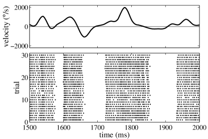
Figure 2: Data from a fly motion sensitive neuron in a natural stimulus setting. Top: a 500 m s  section of a 10 s  angular velocity trace that was repeated 196 times. Bottom: raster plot showing the response to 30 consecutive trials; each dot marks the occurrence of a spike.

For a test on real neurophysiological data, we use recordings from a wide field motion sensitive neuron (H1) in the visual system of the blowfly Calliphora vicina. While action potentials from H1 were recorded, the fly rotated on a stepper motor outside among the bushes, with time dependent angular velocity representative of natural flight. Figure 2 presents a sample of raw data from such an experiment (see Ref. Lewen et al. (2001) for details).

Following Ref. Strong et al. (1998), the information content of a spike train is the difference between its total entropy and the entropy of neural responses to repeated presentations of the same stimulus . The latter is substantially more difficult to estimate. It is called the noise entropy $S_{n}$, since it measures response variations that are uncorrelated with the sensory input. The noise in neurons depends on the stimulus itself—there are, for example, stimuli which generate with certainty zero spikes in a given window of time—and so we write $S_{n|t}$ to mark the dependence on the time $t$ at which we take a slice through the raster of responses. In this experiment the full stimulus was repeated 196 times, which actually is a relatively large number by the standards of neurophysiology. The fly makes behavioral decisions based on $\sim 10-30~{}\mathrm{m}\mathrm{s}$ windows of its visual input Land and Collett (1974), and under natural conditions the time resolution of the neural responses is of order 1 m s  or even less Lewen et al. (2001), so that a meaningful analysis of neural responses must deal with binary words of length $10-30$ or more. Refractoriness limits the number of these words which can occur with nonzero probability (as in our model problem), but nonetheless we easily reach the limit where the number of samples is substantially smaller than the number of possible responses.

Figure 3: Slice entropy vs. sample size. Dashed line on both plots is drawn at the value of $\left.S^{\rm NSB}\right|_{N=N_{\rm max}}$ to show that the estimator is stable within its error bars even for very low $N$. Triangle corresponds to the value of $S^{\rm ML}$ extrapolated to $N\to\infty$ from the four largest values of $N$. First and second panels show examples of word lengths for which $S_{\rm ML}$ can or cannot be reliably extrapolated. $S^{\rm NSB}$ is stable in both cases, shows no $N$ dependent drift, and agrees with $S^{\rm ML}$ where the latter is reliable.

Let us start by looking at a single moment in time, $t=1800~{}\mathrm{m}\mathrm{s}$ from the start of the repeated stimulus, as in Fig. 2. If we consider a window of duration $T=16~{}\mathrm{m}\mathrm{s}$ at time resolution $\tau=2~{}\mathrm{m}\mathrm{s}$ , we obtain the entropy estimates shown in the first panel of Fig. 3. Notice that in this case we actually have a total number of samples which is comparable to or larger than $2^{S_{n|t}}$, and so the maximum likelihood estimate of the entropy is converging with the expected $1/N$ behavior. The NSB estimate agrees with this extrapolation. The crucial result is that the NSB estimate is correct within error bars across the whole range of $N$; there is a slight variation in the mean estimate, but the main effect as we add samples is that the error bars narrow around the correct answer. In this case our estimation procedure has removed essentially all of the sample size dependent bias.

As we open our window to $T=30~{}\mathrm{m}\mathrm{s}$, the number of possible responses (even considering refractoriness) is vastly larger than the number of samples. As we see in the second panel of Fig. 3, any attempt to extrapolate the ML estimate of entropy now requires some wishful thinking. Nonetheless, in parallel with our results for the model problem, we find that the NSB estimate is stable within error bars across the full range of available $N$.

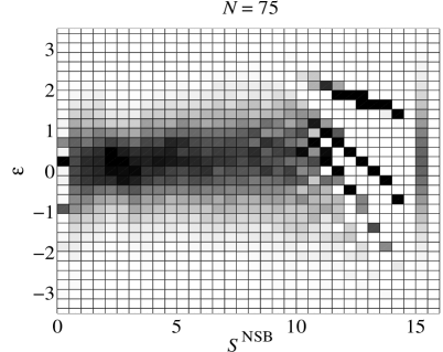
Figure 4: Distribution of the normalized entropy error conditional on $S^{\rm NSB}(N_{\rm max})$ for $N=75$ and $\tau=0.75~{}\mathrm{m}\mathrm{s}$. Darker patches correspond to higher probability. The band in the right part of the plot is the normal distribution around zero with the standard deviation of 1 (the standard deviation of plotted conditional distributions averaged over $S^{\rm NSB}$ is about 0.7, which indicates a non–Gaussian form of the posterior for small number of coincidences Nemenman (2002)). For values of $S^{\rm NSB}$ up to about 12 bits the estimator performs remarkably well. For yet larger entropies, where the number of coincidence is just a few, the discrete nature of the estimated values is evident, and this puts a bound on reliability of $S^{\rm NSB}$.

For small $T$ we can compare the results of our Bayesian estimation with an extrapolation of the ML estimate; each moment in time relative to the repeated stimulus provides an example. We have found that the results in the first panel of Fig. 3 are typical: in the regime where extrapolation of the ML estimator is reliable, our estimator agrees within error bars over a broad range of sample sizes. More precisely, if we take the extrapolated ML estimate as the correct answer, and measure the deviation of $S^{\rm NSB}$ from this answer in units of the predicted error bar, we find that the mean square value of this normalized error is of order one. This is as expected if our estimation errors are random rather than systematic.

For larger $T$ we do not have a calibration against the (extrapolated) $S^{\rm ML}$, but we can still ask if the estimator is stable, within error bars, over a wide range of $N$. To check this stability we treat the value of $S^{\rm NSB}$ at $N=N_{\rm max}=196$ as our best guess for the entropy and compute the normalized deviation of the estimates at smaller values of $N$ from this guess, $\varepsilon=\left[S^{\rm NSB}(N)-S^{\rm NSB}(N_{\rm max})\right]/\delta S^{\rm NSB}(N)$. Again, each moment in time is an example. Figure 4 shows the distribution of these normalized deviations conditional on the entropy estimate with $N=75$; this analysis is done for $\tau=0.75~{}\mathrm{m}\mathrm{s}$, with $T$ in the range between $1.5~{}\mathrm{m}\mathrm{s}$ and $22.5~{}\mathrm{m}\mathrm{s}$. Since the different time slices span a range of entropies, over some range we have $N>2^{S}$, and in this regime the entropy estimate must be accurate (as in the analysis of small $T$ above). Throughout this range, the normalized deviations fall in a narrow band with mean close to zero and a variance of order one, as expected if the only variations with the sample size were random. Remarkably this pattern continues for larger entropies, $S>\log_{2}N=6.2$ bits, demonstrating that our estimator is stable even deep into the undersampled regime. This is consistent with the results obtained in our model problem, but here we find the same answer for the real data.

Note that Fig. 4 illustrates results with $N$ less than one half the total number of samples, so we really are testing for stability over a large range in $N$. This emphasizes that our estimation procedure moves smoothly from the well sampled into the undersampled regime without accumulating any clear signs of systematic error. The procedure collapses only when the entropy is so large that the probability of observing the same response more than once (a coincidence) becomes negligible.

V Discussion

The estimator we have explored here is constructed from a prior that has a nearly uniform distribution of entropies. It is plausible that such a uniform prior would largely remove the sample size dependent bias in entropy estimation, but it is crucial to test this experimentally. In particular, there are infinitely many priors which are approximately (and even exactly) uniform in entropy, and it is not clear which of them will allow successful estimation in real world problems. We have found that the NSB prior almost completely removed the bias in the model problem (Fig. 1). Further, for real data in a regime where undersampling can be beaten down by data the bias is removed to yield agreement with the extrapolated ML estimator even at very small sample sizes (Fig. 3, first panel). Finally and most crucially, the NSB estimation procedure continues to perform smoothly and stably past the nominal sampling limit of $N\sim 2^{S}$, all the way to the Ma cutoff $N^{2}\sim 2^{S}$ (Fig. 4). This opens the opportunity for rigorous analysis of entropy and information in spike trains under a much wider set of experimental conditions.