Precision calculations of atoms with few valence electrons

Abstract

We discuss the possibility of using pair-equations for the construction of the effective Hamiltonian $H_{\rm eff}$ for valence electrons of an atom. The low-energy part of atomic spectrum is found by solving the eigenvalue problem for $H_{\rm eff}$. In this way it is possible to account efficiently for the valence-valence and core-valence correlations. We tested this method on a toy model of a four-electron atom with the core $1s^{2}$. The spectrum obtained with $H_{\rm eff}$ for two valence electrons is in a perfect agreement with the full configuration interaction for all four electrons.

Introduction

The reliable and accurate ab initio methods for atomic calculations are necessary not only for atomic physics and quantum chemistry, but also for application of atomic physics to the investigation of the fundamental interactions. For example precision calculations of Cs were necessary to test electroweak theory on the level of radiative corrections at low energy (see [1] and references therein). Recent search for the possible variation of the fine structure constant $\alpha$ [2] in space-time also required large-scale atomic calculations [3].

At present there are several widely used methods for calculations of many-electron atoms. For atoms with one valence electron above the core the many-body perturbation theory (MBPT) appears to be very effective [4]. For the atoms with more than one valence electrons the accuracy of the conventional MBPT techniques is not satisfactory mainly because of the poor convergence of the MBPT for the valence-valence correlations. Because of that non-perturbative methods are usually preferable [5, 6, 7, 8, 9]. However, the core-valence correlations can still be effectively treated with MBPT. Because of that it was suggested to combine MBPT for the core-valence correlations with the configuration interaction (CI) for valence-valence correlations within the CI+MBPT method [10].

In this method CI calculation for valence electrons is done with the effective Hamiltonian $H_{\rm eff}$. This Hamiltonian accounts for core polarization and screening of the two-electron interaction between valence electrons. It may be formed within the Brillouin-Wigner variant of MBPT. In practice most of the calculations were done within the second order MBPT [11, 12, 13, 14, 15]. The operator $H_{\rm eff}$ is defined for valence electrons only. Therefore, CI+MBPT method is equivalent to the multi-reference MBPT with the model space coinciding with the whole valence space. The use of the Brillouin-Wigner variant of MBPT allows to avoid problems with intruder states, but leads to the energy-dependent effective Hamiltonian [16, 17].

CI+MBPT method has several important limitations:

1. The number of valence electrons should not be large. The accuracy of the CI method rapidly decreases when this number exceeds 3 or 4.

2. Only the lower part of the valence spectrum can be presented accurately. For the energies above the excitation energy of the core the effective Hamiltonian has poles and results of the CI+MBPT method may become unreliable [18].

3. The accuracy of the calculations is limited because the effective Hamiltonian does not account for the higher order core-valence correlations. With the second order effective Hamiltonian the typical accuracy for the transition frequencies is of the order of a percent.

The first two limitations are intrinsic to the method. In order to address the third one it is necessary to go beyond the second order MBPT. One obvious way to do this is the order-by-order approach. However, it is known that for atoms with one valence electron the third order calculations are often even less accurate than the second order ones. Besides, for atoms with more than one valence electron the third order is already too complicated for practical use.

The arguments given above lead us to one of the variants of the all-order methods. The coupled-cluster method is one of the most widely used [5]. It gives the nonlinear system of equations for cluster amplitudes. In order to truncate this system it is often restricted to SD excitations. The linearized version of the coupled-cluster equations in the SD-approximation are also known as pair equations, or SD-method [19]. It was used for the calculations of the atoms with one valence electron and proved to be significantly more accurate than the second order MBPT [20]. So, we suggest to use CI+SD method instead of CI+MBPT for the calculations of the atoms with few valence electrons.

In order to use the SD-method for the effective Hamiltonian, we developed the Brillouin-Wigner variant of these equations and added equations for the two-electron amplitudes, which were absent in the one-electron atoms. That allowed us to form the effective Hamiltonian for valence electrons in SD-approximation.

As a test system for the CI+SD method we study a toy model of a 4-electron atom with two valence electrons above the core $1s^{2}$. We use a very short basis set, for which the 4-electron full CI is possible. That allows to test the method without addressing such questions as saturation of the basis set and the role of the Breit interaction, which we do not include here. This model was recently considered in [21] and appeared useful for the study of the higher orders in the residual core-valence interaction.

1 Effective Hamiltonian

It is well known that if we split the total many-electron Hilbert space in two subspaces $P$ and $Q$, $P+Q=1$, the full Schrödinger equation can be equivalently rewritten in a following form:

$$\Psi=P\Psi+Q\Psi\equiv\Phi+\chi,$$ (1)

$$\left(PHP+\Sigma(E)\right)\Phi=E\Phi,$$ (2)

where

$$\Sigma(E)=(PHQ)\ {R}_{Q}(E)\ (QHP),$$ (3)

$$R_{Q}(E)=(E-QHQ)^{-1}$$ (4)

Eq. (2) shows, that the effective Hamiltonian in the subspace $P$ has the form:

$$H_{\rm eff}(E)\equiv PHP+\Sigma(E).$$ (5)

Note that this $P,Q$ expansion is formally equivalent, for example, to the exclusion of the small component from the Dirac equation. For practical purposes the particular choice of the subspace $P$ is very important. For atoms with few valence electrons it is natural to associate this subspace with the valence one. In other words $P$ subspace corresponds to the frozen-core approximation $P=P_{\rm FC}$. This means that core-core and core-valence correlations are accounted for on the stage of formation of the operator $H_{\rm eff}$, while all valence correlations are treated explicitly when solving Eq. (2).

Of course, for many-electron atoms the exact form of the operator $R_{Q}(E)$ is not known and some approximations should be used. In principle, MBPT gives consistent procedure for finding an order-by-order expansion of this operator in powers of the residual two-electron interaction. In the lowest (second) order $R_{Q}(E)$ is substituted by $R_{Q}^{0}(E)=(E-QH_{0}Q)^{-1}$, where $H_{0}$ is a one-electron operator. This leads to the second order effective Hamiltonian for valence electrons, which was used in calculations [11, 12, 13, 14]. The complete form of the third order expansion for $H_{\rm eff}$ is still unknown and is probably to complicated for practical use.

The most simple and compact variant of the MBPT expansion corresponds to the choice, when $H_{0}$ is equal to the Dirac-Fock operator of the core $H^{\rm DF}_{\rm core}$. At least for atoms with one or two valence electrons this may be also an optimal choice [21]. For more valence electrons one may want to include, at least partly, the field of the valence electrons in $H_{0}$. This leads to many new terms in the MPBT expansion [10], but gives better initial approximation. In our calculations we use the Dirac-Fock code [22], which allows for the flexible choice of the self-consistent field.

In the end of this section we want to mention that sometimes the whole wave function (1) is needed. Then we can recover it from the solution of (2) with the help of relation:

$$\Psi=\Phi+\chi=\left(1+R_{Q}(E)\ (QHP)\right)\Phi.$$ (6)

We again can use MBPT expansion for $R_{Q}(E)$ here. If we need $\chi$ to calculate some atomic amplitudes, we can use Eq. (6) to define corresponding effective operator in the subspace $P$. For the effective operators one can use the random phase approximation with additional two-electron terms instead of the order-by-order MBPT [23]. This technique was used in calculations of $E1$-transitions [13], polarizabilities [24], and hyperfine constants [18].

2 SD-method for the effective Hamiltonian

As we mentioned above, the accuracy of the CI+MBPT method is limited because of the neglect of the higher order corrections to $H_{\rm eff}$. The SD-method allows to sum to all orders the MBPT terms, which correspond to the one and two holes in the core in all intermediate cross-sections of the Goldstone diagrams. Technically this leads to the substitution of the one- and two-electron matrix elements in $H_{\rm eff}$ with corresponding SD-amplitudes.

The explicit form of the SD-equation depends on the choice of the one-electron operator $H_{0}$, which is used for the initial approximation. The simplest form corresponds to $H_{0}=H^{\rm DF}_{\rm core}$, which we assume below. We expect that in analogy with the CI+MBPT, this variant of the CI+SD method should be good at least for one- and two-electron atoms.

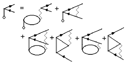
Figure 1: Graphic form of the SD-equation for the one-electron core amplitude. Wavy line corresponds to Coulomb interaction, double line denotes two-electron SD-amplitude, and double line with the circle denotes one-electron SD-amplitude.

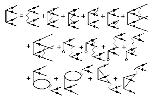
Figure 2: Graphic form of the SD-equation for the two-electron core amplitude.

The system of equations for SD-amplitudes splits in three parts. The first subsystem includes only amplitudes for core excitations. Therefore, these amplitudes do not depend on core-valence and valence amplitudes and should be solved first [19]. The graphic representation of this subsystem is shown in Fig. 1 and 2. Note that all equations are presented in a form, suitable for iterative solution. At first iteration we put all SD-amplitudes on the right-hand-sides to zero. That leaves the single non-zero term in the equation for the two-electron SD-amplitude Fig. 2. As a result we get non-zero two-electron amplitude, but the one-electron SD-amplitude is still zero. On the next iteration both right-hand-sides in Fig. 1 and 2 are non-zero.

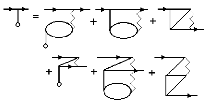
Figure 3: SD-equation for the one-electron valence amplitude.

On the next step the one electron valence amplitudes and two-electron core-valence amplitudes should be found from the system of equations shown in Fig. 3 and 4. It is seen that they depend on each other and on the core amplitudes, which were found on the previous step. This system again can be solved iteratively. Iteration processes on the first and the second steps converge rather rapidly because the energy denominators for all diagrams are large, because they include the excitation energy of the core. The latter grows with the number of valence electrons, so we can expect faster convergence for the atoms with more valence electrons.

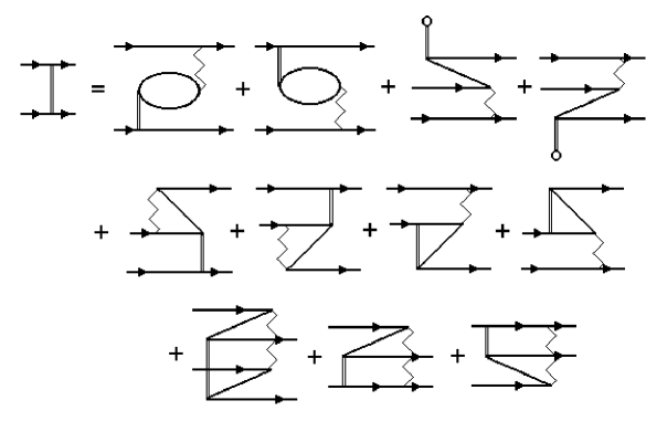
Figure 5: Diagramatic expression for the two-electron valence amplitude.

The one-electron valence SD-amplitudes, which are found from the equations on Fig. 3 can be already used for the construction of $H_{\rm eff}$. However, on this step we still do not have two-electron valence amplitudes. These can be found by calculating diagrams from Fig. 5. Corresponding diagrams depend only on the amplitudes, which are already found on previous steps, so we can calculate two-electron valence SD-amplitudes in one run. Therefore, the third step is rather simple and this is the only new step, which was not used in calculations of one-electron atoms [19]. It means that the SD-method is easily generalized for the many-electron case.

There are several questions, which we did not address above. First is the energy dependence of the SD-amplitudes. That can be accounted for in a same way, as it was done in CI+MBPT method. Second, we prefer to have Hermitian effective Hamiltonian, while the valence SD-amplitudes as given by Fig. 3 and 5 are non-symmetric. Thus, we need to symmetrize them somehow. These questions will be discussed elsewhere in detail. Here we prefer to give an example of the application of the CI+SD method to a model system, which can be solved ‘exactly’ and the accuracy of the CI+SD approximation can be therefore well controlled and compared to that of the CI+MBPT method.

3 Toy model

Here we consider the atom with $Z=6$ and 4 electrons in a very short basis set of 14 orbitals $1-4s_{1/2}$, $2-4p_{j}$, and $3,4d_{j}$. Because of such a short basis set, we can not compare our results with the physical spectrum of C III. Instead, we can do the full CI for all 4 electrons and use it as an ‘exact’ solution. Alternatively, we can consider the same atom as a two-electron system with the core $[1s^{2}]$. In this case we can use both CI+MBPT and SI+SD methods and compare their results with the known ‘exact’ solution.

As an even simpler test systems we can also consider the same system with 2 and 3 electrons. The core equations Fig. 1 and 2 are the same for all three cases. After they are solved, we can immediately find the correlation correction to the core energy by calculating two diagrams from Fig. 6. The same correction can be found with the help of the full CI for two electrons. Note that SD-method for the two electron system is exact, so both result should coincide. In this way we can effectively check the system of equations for core amplitudes.

The iterative procedure for the core SD-equations converges in three steps and the core correlation energy $\delta E_{\rm core}$ in atomic units is given by:

Iteration	$\delta E_{\rm core}$	Difference
1	$-0.006051$	$-0.006051$
2	$-0.006278$	$-0.000228$
3	$-0.006282$	$-0.000004$
Full CI	$-0.006280$	$+0.000002$

The difference $2\cdot 10^{-6}$ a.u. between the full CI and SD results is two orders of magnitude smaller than the error of the second order MBPT, which corresponds to the first iteration and is probably due to the numerical accuracy (we store radial integrals in the CI code [25] as real*4 numbers).

When core SD-amplitudes are found, we find one-electron valence amplitudes from the system of equations from Fig. 3 and 4. This allows us to form $H_{\rm eff}$ for one electron above the core and find the spectrum of the three-electron system. These results are compared to the three-electron full CI in Table 1.

Finally, we calculate two-electron valence SD-amplitudes and form two-electron effective Hamiltonian. Two-electron full CI with $H_{\rm eff}$ is compared with four-electron full CI in Table 2.

4 Discussion

SD-method for the system with valence electrons is not exact even for the two-electron core [19]. Therefore we can not expect exact agreement between SD and full CI results. We still expect higher accuracy for the CI+SD method than for CI with the second order $H_{\rm eff}$. Tables 1 and 2 show that this is the case. For the one-electron case both the maximum and the average error decreases by the factor of 3 to 4. For the two-electron case the error decreases even stronger.

Moreover, if the third order corrections are added to the one-electron SD-amplitudes, as was suggested in [26], the accuracy rises by almost another order of magnitude. If we include one-electron third order corrections to the two-electron effective Hamiltonian, the error in comparison to the SD-approximation even grows. The total number of the third order two-electron diagrams is very large and at present we are able to include them only partly. It is seen from the Table 2 that this improves the accuracy a bit in comparison to the SD-approximation. However, we see that there are no dominant third order diagrams, which are not included in the SD-approximation. In fact there are many contributions of the same order of magnitude and of different signs, so that they strongly cancel each other. It is possible that complete third order correction would give even better accuracy, but any partial account of the third order may be dangerous.

We conclude that in the many-electron case there is no point in including only one-electron third order corrections to the effective Hamiltonian or any other subset of the complete set of the third order terms. That probably means that for a more complicated atom it may be too difficult to improve SD-results by including the third order corrections. Note that for more than two valence electrons there will be also three-electron terms in the effective Hamiltonian.

We see that for the simple model system considered here the SD-approximation for the effective Hamiltonian appears to be few times more accurate than the second order MBPT. It is still not obvious that this will hold for the more complicated systems. As we saw above, the two-electron core is a special case for the SD method as the latter allows to obtain the core energy exactly here. The advantage of the model considered here is that we can compare results with the full-electron calculation, which is impossible in the general case. The computational expenses for a full scale atomic calculations within CI+SD method are significantly higher that in CI+MBPT(II), but are still lower than in CI+MBPT(III).

The author is grateful to E. Eliav, T. Isaev, W. Johnson, N. Mosyagin, S. Porsev, and A. Titov for valuable discussions. This work was supported by RFBR, grant No 02-02-16387.

Table 1: Comparison of different one-electron approximations with three-electron full CI. Three-electron transition frequencies and the errors for one-electron calculations are given in cm^-1. One-electron calculations include Dirac-Fock (DF), Dirac-Fock with the second order self-energy correction (MBPT), SD-approximation, and SD with third order corrections (SD+III). Averaged absolute value of the errors and maximum errors are given at the bottom.

Level	Full CI	One-electron approximations
		DF	MBPT	SD	SD+III
$2s_{1/2}$	0.0	0.0	0.0	0.0	0.0
$2p_{1/2}$	64870.1	329.9	46.1	16.0	2.2
$2p_{3/2}$	64999.6	328.6	45.2	15.1	1.5
$3s_{1/2}$	302411.3	-256.1	-49.5	-11.1	-1.2
$3p_{1/2}$	319727.1	-189.4	-40.8	-8.1	-1.1
$3p_{3/2}$	319765.1	-189.7	-40.9	-8.4	-1.4
$3d_{3/2}$	324342.0	-284.9	-61.7	-13.9	-2.2
$3d_{5/2}$	324351.2	-284.9	-61.7	-13.8	-2.2
av. err.		266	50	12	1.7
max. err.		330	50	16	2.2

Table 2: Comparison of two-electron approximations with four-electron full CI. Two-electron full CI is made for initial Hamiltonian and for effective Hamiltonians calculated within second order MBPT, SD, and SD with third order corrections (SD+III). In the latter case either one-electron or one-electron and partly two-electron terms were included.

Level	Full CI	Two-electron approximations
		CI	MBPT	SD	SD+III
${}^{1}S_{0}(2s^{2})$	0.0	0.0	0.0	0.0	0.0	0.0
${}^{3}P_{0}(2s2p)$	52535.9	222.0	31.6	5.0	-4.9	1.9
${}^{3}P_{1}(2s2p)$	52569.7	221.9	31.8	5.2	-4.7	2.1
${}^{3}P_{2}(2s2p)$	52637.5	221.7	31.8	5.7	-4.2	2.6
${}^{1}P_{1}(2s2p)$	104969.2	865.4	80.3	-19.9	-30.1	9.7
${}^{3}P_{0}(2p^{2})$	138303.7	1016.9	111.0	-1.8	-22.0	0.4
${}^{3}P_{1}(2p^{2})$	138337.0	1016.3	110.7	-2.2	-22.4	-0.2
${}^{3}P_{2}(2p^{2})$	138402.9	1015.3	110.4	-2.4	-22.6	-0.2
${}^{1}D_{2}(2p^{2})$	147954.8	698.6	70.1	-3.5	-21.5	9.7
${}^{1}S_{0}(2p^{2})$	186561.7	845.5	63.7	-14.7	-45.4	13.7
${}^{3}S_{1}(2s3s)$	239752.9	79.5	11.7	13.7	22.0	8.4
${}^{1}S_{0}(2s3s)$	251971.5	59.8	0.9	2.0	9.7	1.6
av. err.	0	569	60	7	19	5
max. err.	0	1017	111	20	45	14

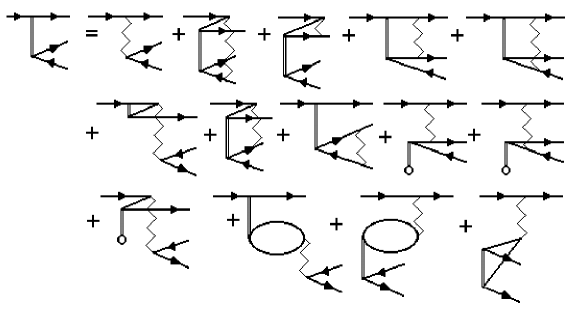
Figure 4: SD-equation for the two-electron core-valence amplitude.

Figure 6: Core correlation energy in the SD-approximation.

References

- [1] K. Hagiwara et al., Phys. Rev. D 66, 010001 (2002).
- [2] J. K. Webb et al., Phys. Rev. Lett. 87, 091301 (2001).
- [3] V. A. Dzuba, V. V. Flambaum, M. G. Kozlov, and M. Marchenko, Phys. Rev. A 66, 022501 (2002).
- [4] M. S. Safronova, A. Derevianko, and W. R. Johnson, Phys. Rev. A 58, 1016 (1998).
- [5] J. Paldus, Methods in Computational Molecular Physisc (NATO Advanced Study Institute, New-York, 1992), vol. 293 of Ser. B: Physics, p. 99, Ed. S Wilson and G H F Diercksen.
- [6] F. A. Parpia, C. Froese Fischer, and I. P. Grant, Comput. Phys. Commun. 94, 249 (1996).
- [7] E. Eliav et al., Phys. Rev. A 53, 3926 (1996).
- [8] E. Eliav and U. Kaldor, Phys. Rev. A 53, 3050 (1996).
- [9] N. S. Mosyagin, E. Eliav, A. V. Titov, and U. Kaldor, J. Phys. B 33(4), 667 (2000).
- [10] V. A. Dzuba, V. V. Flambaum, and M. G. Kozlov, Phys. Rev. A 54, 3948 (1996).
- [11] M. G. Kozlov and S. G. Porsev, Sov. Phys.–JETP 84, 461 (1997).
- [12] V. A. Dzuba and W. R. Johnson, Phys. Rev. A 57, 2459 (1998).
- [13] S. G. Porsev, M. G. Kozlov, and Y. G. Rahlina, JETP Lett. 72, 595 (2000).
- [14] M. G. Kozlov, S. G. Porsev, and W. R. Johnson, Phys. Rev. A 64, 052107 (2001).
- [15] I. M. Savukov and W. R. Johnson, Phys. Rev. A 65, 042503 (2002).
- [16] I. Hubac and S. Wilson, J. Phys. B 33, 365 (2000).
- [17] M. G. Kozlov and S. G. Porsev, Opt. Spectrosc. 87, 352 (1999).
- [18] S. G. Porsev, Y. G. Rakhlina, and M. G. Kozlov, J. Phys. B 32, 1113 (1999).
- [19] S. A. Blundell, W. R. Johnson, Z. W. Liu, and J. Sapirstein, Phys. Rev. A 40, 2233 (1989).
- [20] M. S. Safronova and W. R. Johnson, Phys. Rev. A 62, 022112/1 (2000).
- [21] M. G. Kozlov, Opt. Spectrosc. 95, to be published (2003).
- [22] V. F. Bratsev, G. B. Deyneka, and I. I. Tupitsyn, Bull. Acad. Sci. USSR, Phys. Ser. 41, 173 (1977).
- [23] V. A. Dzuba, M. G. Kozlov, S. G. Porsev, and V. V. Flambaum, Sov. Phys.–JETP 87, 885 (1998).
- [24] M. G. Kozlov and S. G. Porsev, Eur. Phys. J. D 5, 59 (1999).
- [25] S. A. Kotochigova and I. I. Tupitsyn, J. Phys. B 20, 4759 (1987).
- [26] M. S. Safronova, W. Johnson, and A. Derevianko, Phys. Rev. A 60, 4476 (1999).