Variational RPA for the Mie resonance in jellium

Abstract

The surface plasmon in simple metal clusters is red-shifted from the Mie frequency, the energy shift being significantly larger than the usual spill-out correction. Here we develop a variational approach to the RPA collective excitations. Using a simple trial form, we obtain analytic expressions for the energy shift beyond the spill-out contribution. We find that the additional red shift is proportional to the spill-out correction and can have the same order of magnitude.

I Introduction

Simple metal clusters exhibit a strong peak in their optical response that corresponds to a collective oscillation of the valence electrons with respect to a neutralizing positively charged background. Classically, the frequency of the oscillation is given by the Mie resonance formula[1, 2],

$$\omega_{\rm Mie}^{2}={4\pi ne^{2}\over 3m}$$ (1)

where $n$ is the density of a homogeneous electron gas. Quantum finite size effects lead to a red shift of this frequency as well as to a redistribution of the oscillator strength ($f$) into closely lying dipole states. Moments of the oscillator strength distribution $M_{k}=\sum_{i}\omega_{i}^{k-1}f_{i}$ provide useful information. The first moment $M_{1}$, which measures the integral of the $f$-distribution, equals the number of electrons (Thomas-Reiche-Kuhn sum rule). The mean square frequency $\langle\omega^{2}\rangle=M_{3}/M_{1}$ is given by the overlap integral of the positive ionic charge distribution and the exact ground state electronic density[2]. Within an ionic background approximated by a jellium sphere, the mean square frequency is thus exactly related to the square Mie frequency by

$$\langle\omega^{2}\rangle=\omega_{\rm Mie}^{2}\left(1-\frac{\Delta N}{N}\right)$$ (2)

where $\Delta N/{N}$ is the fraction of electrons in the ground state that is outside the jellium sphere radius. We called the corresponding energy shift $\Delta\omega_{so}$ (“spill-out”):

$$\Delta\omega_{so}=\omega_{\rm Mie}(1-\sqrt{1-\Delta N/N})$$ (3)

The actual red shifts are considerably larger than this. For sake of illustrating the discussion let us consider the sodium cluster Na${}^{+}_{21}$ for which detailed photoabsorption data is available[3, 4, 5, 6, 7]. The Mie frequency is at 3.5 eV, taking the density corresponding to $r_{s}=3.93$ a.u., while the measured resonance is a peak 2.65 eV having width of about 0.3 eV (FWHM). Thus there is a red shift of 24%, which may be compared with a 9% red shift predicted by eq. (3) using jellium wave functions. To a large extent clusters with a “magic” number of valence electrons behave optically as close shell spherical jellium spheres. The experimental photoabsorption spectra for these clusters are well described within the linear response theory using either the time-dependent local-density approximation (TDLDA)[8, 9, 10] or the random phase approximation with exact exchange (RPAE)[11, 12]. Red shifts of 14% and 18% are predicted by time-dependent density functional theory [13] and by the random phase approximation [11, 12], respectively. The oscillator strength distributions in the RPA calculations are typically dominated by a few close states that exhaust almost all of the sum rule. It is this concentration of strength, which we can identify as a dipole surface plasmon, that will be of interest in this paper. It is worth of note that singling out a collective state is not always possible even in small clusters. Whenever the collective state lies within a region of high level density, there is a strong fragmentation into p-h states (Landau damping) and several excited states may share evenly the strength. We will deal with this problem of the definition of the collective state later by proposing a model in which there is no particle-hole fragmentation.

Anharmonic effects in metallic clusters were studied recently by Gerchikov, et al., [14] making use of a coordinate transformation to separate center of mass (c.m.) and intrinsic motion. The authors show that in absence of coupling between c.m. motion and intrinsic excitations the surface plasmon associated with a jellium sphere has a single peak which is red-shifted with respect to the Mie frequency by the spill-out electrons, Eq. (3). Turning on the coupling yields a further red shift which indeed is larger in magnitude than the spill-out contribution. Concomitantly, there is a partial transfer of strength into states of higher energy preserving the sum rule, Eq. (2). The approach requires the spectrum of excitations in the intrinsic coordinates, which were obtained by projection on the computed wave functions of the numerical RPAE.

Another interesting approach to the coupling between the collective and noncollective degrees of freedom was developed by Kurasawa, et al., [15], following the Tomonaga expansion of the Hamiltonian. The collective coordinate is taken as the cm coordinate, as in ref. [14], and the coefficients of the harmonic terms in the Hamiltonian yield Eq. (2) for the frequency. The authors derive expressions for the coupling terms in the Hamiltonian and use them to estimate the variance of the Hamiltonian in the collective state. They find that the variance decreases with size of the cluster as $1/R$, where $R$ is the radius of the ion distribution. Both the width of the Mie and its shift are obviously related to the variance of H, but further assumptions are needed to make a quantitative connection.

In the present paper we wish to find an analytic estimate of the red shift, keep as far as possible the ordinary formulation of RPA, and not singling out a collective state in the Hamiltonian. Our approach will be a variational RPA theory, which we present in the next section. The rest of the paper is organized as follows. In Section III we apply the formalism to a system of interacting electrons. The model Hamiltonian describes interacting electrons confined in a pure harmonic potential, whereas the perturbation corrects for the jellium confinement. The model RPA solution is derived analytically and first and second order corrections of the frequency shift are given.

II Variational RPA

In this section, we establish our notation for the RPA theory of excitations and develop a variational expression for perturbations to the collective excitation frequency. The perturbation behaves somewhat differently in RPA than in conventional matrix Hamiltonians because the RPA operator is not Hermitean.

As usual, the starting point is a mean field theory whose ground state is represented by an orbital set ${\phi_{i}}$ satisfying the orbital equations

$$h[\rho_{0}]\phi_{i}=\epsilon_{i}\phi_{i}$$ (4)

where $\rho_{0}=\sum_{i}|\phi_{i}(r)|^{2}$. The RPA equations are obtained by considering small deviations from the ground state,

$$\phi_{i}\rightarrow\phi_{i}+\lambda(x_{i}e^{-i\omega t}+y_{i}e^{i\omega t}).$$ (5)

Here $x_{i},y_{i}$ are vectors in whatever space ($r$-space,orbital occupation number,…) is used to represent $\phi_{i}$. The RPA equations can be expressed as

$$(h[\rho_{0}]-\epsilon_{i})x_{i}+\delta\rho*{\delta h\over\delta\rho}*\phi_{i}=\omega x_{i}$$ (6)

$$-(h[\rho_{0}]-\epsilon_{i})y_{i}-\delta\rho*{\delta h\over\delta\rho}*\phi_{i}=\omega y_{i}$$

where the transition density $\delta\rho$ is defined by

$$\delta\rho=\sum_{i}\phi_{i}(x_{i}+y_{i})$$

and the symbol $*$ denotes an operator or matrix multiplication. Eq. (6) represents linear eigenvalue problem for a nonhermitean operator $R$ and the vector $|z\rangle=(x_{1},y_{1},x_{2},y_{2},...)$. We will write the equations compactly as

$$R|z\rangle=\omega|z\rangle.$$

For a nonhermitean operator, the adjoint vector $\langle z|$ is defined as the eigenvector of the adjoint equation, $\langle z|R=\omega\langle z|.$ From the symmetry of $R$ it is easy to see that it is given by $\langle z|=(x_{1},-y_{1},x_{2},-y_{2},...)^{\dagger}$.

We now ask how to construct a perturbation theory starting from the zero-order wave function $|z_{0}\rangle$ that is the solution of an unperturbed $R_{0}$ with eigenfrequency $\omega_{0}$. If we had the complete spectrum of $R_{0}$, the perturbation series for $R=R_{0}+\Delta R$ could be written down in the usual way,

$$|z\rangle=|z_{0}\rangle+\sum_{\alpha}|z_{\alpha}\rangle{\langle z_{\alpha}|\Delta R|z\rangle\over\omega_{0}-\omega_{\alpha}},$$

etc. This is in fact what is done in ref. [14]. However, this requires diagonalizing $R_{0}$ which in general can only be done numerically.

Instead we shall estimate the energy perturbation using a variational expression for the frequency,

$$\omega=\min_{w}{\langle z_{0}+\lambda w|R|z_{0}+\lambda w\rangle\over\langle z_{0}+\lambda w|z_{0}+\lambda w\rangle},$$ (7)

where $|w\rangle$ is a vector to be specified later and $\lambda$ is to be varied to minimize the expression. Carrying out the variation and assuming that the perturbation is small, the value of $\lambda$ at the minimum is given by

$$\lambda\approx-{\langle z_{0}|R|w\rangle-\omega_{0}\langle z_{0}|w\rangle\over\langle w|Rw\rangle-\omega_{1}\langle w|w\rangle}$$ (8)

and the energy shift is

$$\omega\approx\omega_{0}+\langle z_{0}|\Delta R|z_{0}\rangle-{(\langle z_{0}|Rw\rangle-\omega_{1}\langle z_{0}|w\rangle)^{2}\over\langle w|Rw\rangle-\omega_{1}\langle w|w\rangle}.$$ (9)

Here, $\omega_{1}\equiv\langle z_{0}|R|z_{0}\rangle=\omega_{0}+\langle z_{0}|\Delta R|z_{0}\rangle.$

The next question is how to choose the perturbation $|w\rangle$. With ordinary Hamiltonians, one can construct a two-state perturbation theory using the vector obtained by applying $\Delta R$ to the unperturbed vector, $|w\rangle=\Delta R|z_{0}\rangle$. However, we will see in the next section that this fails completely for the RPA operator. Instead, we will find that an approximation that gives qualitatively acceptable results can be made by taking only the $x$-component of the vector defined by applying $\Delta R$ to $|z_{0}\rangle$.

III Collective limit of the surface plasmon

We apply the RPA variational perturbation theory derived in the previous section to the surface plasmon of small metal clusters. We write the single particle Hamiltonian as

$$h = h_{0}+\Delta V(r),$$ (10)

$$h_{0} = -\frac{\hbar^{2}}{2m}\nabla^{2}+\frac{1}{2}m\omega_{0}^{2}r^{2}+v*\rho_{0},$$ (11)

where $v*\rho_{0}$ is the mean field potential,

$$v*\rho_{0}=\int v(r,r^{\prime})\rho_{0}(r^{\prime})\,d^{3}r^{\prime}.$$ (12)

Here $v$ is the electron-electron interaction, which may contain an exchange-correlation contribution from density functional theory. In this paper, we throughout use the jellium model for the ionic background, and also assume that the ion and the electron densities are both spherical. $\omega_{0}$ and $\Delta V(r)$ are then given by $\omega_{0}=Ze^{2}/mR^{3}$ and

$$\Delta V(r)=\left[-\frac{Ze^{2}}{r}-\left(-\frac{3}{2}+\frac{r^{2}}{2R^{2}}\right)\frac{Ze^{2}}{R}\right]\,\theta(r-R),$$ (13)

respectively, $R$ being the sharp-cutoff radius for the ion distribution.

The RPA equations can be solved exactly for the Mie resonance if $h$ is replaced by $h_{0}$. The solution is

$$|z_{0}\rangle\equiv\left(\matrix{x\cr y\cr}\right)=-\sqrt{\frac{m\omega_{0}}{2N}}\left(\matrix{z\phi\cr-z\phi\cr}\right)+\sqrt{\frac{1}{2Nm\omega_{0}}}\left(\matrix{\partial_{z}\phi\cr\partial_{z}\phi\cr}\right),$$ (14)

associated with the eigenfrequency $\omega_{0}$. Notice that the eigenfrequency $\omega_{0}$ is the same as the harmonic oscillation frequency in Eq. (11), agreeing with the Kohn’s theorem [16, 17, 18, 19, 20].

To prove that the collective solution (14) satisfies the RPA equation, we use the following identity which results from the Hartree-Fock equation,

$$(h-\epsilon)(\hat{A}\phi)=[h,\hat{A}]\phi.$$ (15)

Here $\hat{A}$ is any one body operator. This yields

$$(h_{0}-\epsilon)(z\phi) = -\frac{1}{m}\partial_{z}\phi,$$ (16)

$$(h_{0}-\epsilon)(\partial_{z}\phi) = -(m\omega_{0}^{2}z+(v*\partial_{z}\rho_{0}))\phi.$$ (17)

In the last step, we used the fact that the interaction $v$ is translationally invariant. Notice that the transition density is proportional to $\partial_{z}\rho_{0}$ for the collective solution (14). The second term in Eq. (17) is thus exactly canceled by the residual interaction term in the RPA equations, proving that the collective ansatz (14) is indeed the eigenfunction of the RPA matrix $R_{0}$ with the eigenvalue $\omega_{0}$.

The familiar formula relating the red-shift to the electron spill-out probability can be recovered from the expectation value of the original RPA matrix,

$$\frac{(z_{0}|Rz_{0})}{(z_{0}|z_{0})}=\omega_{0}+\Delta\omega.$$ (18)

However, the wave function $z_{0}$ must be taken with the collective ansatz applied to the Hamiltonian $h$. This is different from the $z_{0}$ defined in Eq. (14), which was based on the Hamiltonian $h_{0}$. In the following, we have no further use for the original $z_{0}$ and we will use the same name here. Applying the RPA operator $R$ to $z_{0}$, we find

$$R|z_{0}\rangle=\omega_{0}|z_{0}\rangle+|u\rangle,$$ (19)

where $u$ is given by

$$|u\rangle=-\sqrt{\frac{1}{2Nm\omega_{0}}}\,\frac{1}{r}\frac{d\Delta V}{dr}\left(\matrix{z\phi\cr-z\phi\cr}\right).$$ (20)

The expectation value eq. (18) then reduces to

$$\Delta\omega=(z_{0}|u)=-\omega_{0}\,\frac{\Delta N}{2N},$$ (21)

with

$$\Delta N=\int^{\infty}_{R}4\pi r^{2}dr\,\rho_{0}(r).$$ (22)

Eq. (21) is just the well-known spill-out formula, Eq.(3), to the first order in $\Delta N/N$.

IV Evaluation of the integrals

We now consider the frequency shift in the second order perturbation. Obvious possibilities for the perturbation are $w_{0}\equiv(y,x)$ and $u$, but we find that neither produces a significant energy shift. The problem with $u$ is that the $x$ component is tied to the $y$ component in Eq. (20). In fact, the energetics are such the $y$ perturbation is much less than the $x$ perturbation. In order to avoid this undesirable feature, as we mentioned in Sec. II, we simply take the $x$ component of $u$ for the perturbation. That is, we use

$$|\tilde{u}\rangle\equiv\frac{1}{r}\frac{d\Delta V}{dr}\left(\matrix{z\phi\cr 0\cr}\right)=\frac{\partial\Delta V}{\partial z}\left(\matrix{\phi\cr 0\cr}\right),$$ (23)

for the $|w\rangle$ in the variational formula (7). With this perturbed wave function, after performing the angular integration, we find the three integrals in the formula to be

$$\langle z_{0}|\tilde{u}\rangle = -\sqrt{\frac{m\omega_{0}}{2N}}\frac{4\pi}{3}\int^{\infty}_{R}r^{3}dr\,\frac{d\Delta V}{dr}\,\rho_{0}(r)$$ (25)

$$+\sqrt{\frac{1}{2Nm\omega_{0}}}\frac{2\pi}{3}\int^{\infty}_{R}r^{2}dr\,\frac{d\Delta V}{dr}\frac{d\rho_{0}}{dr},$$

$$\langle\tilde{u}|\tilde{u}\rangle = \frac{4\pi}{3}\int^{\infty}_{R}r^{2}dr\,\left(\frac{d\Delta V}{dr}\right)^{2}\rho_{0}(r),$$ (26)

$$\langle z_{0}|R\tilde{u}\rangle = \omega_{0}\langle z_{0}|\tilde{u}\rangle+\langle u|\tilde{u}\rangle=\omega_{0}\langle z_{0}|\tilde{u}\rangle-\sqrt{\frac{1}{2Nm\omega_{0}}}\,\langle\tilde{u}|\tilde{u}\rangle.$$ (27)

In deriving Eq.(27), we have used Eq.(19). We also need to compute $\langle\tilde{u}|R|\tilde{u}\rangle$ in order to estimate the energy shift. Neglecting the residual interaction in the RPA operator $R$, this is expressed as

$$\langle\tilde{u}|R|\tilde{u}\rangle\sim\langle\frac{\partial\Delta V}{\partial z}\phi|h-\epsilon|\frac{\partial\Delta V}{\partial z}\phi\rangle.$$ (28)

We use Eq.(15) to evaluate the action of the Hamiltonian $h$ onto the $\tilde{u}$. This yields

$$(h-\epsilon)\,|\frac{\partial\Delta V}{dz}\phi\rangle=-\frac{1}{2m}\left[\left(\nabla^{2}\frac{\partial\Delta V}{\partial z}\right)+2\left(\nabla\frac{\partial\Delta V}{\partial z}\right)\cdot\nabla\right]\,|\phi\rangle.$$ (29)

Notice that the first term vanishes for the jellium model (13). We thus finally have

$$\langle\tilde{u}|R|\tilde{u}\rangle = -\frac{1}{2m}\int d^{3}r\,\frac{\partial\Delta V}{\partial z}\left(\nabla\frac{\partial\Delta V}{\partial z}\right)\cdot\nabla\rho_{0},$$ (30)

$$= -\frac{1}{2m}\frac{4\pi}{3}\int^{\infty}_{R}r^{2}dr\,\frac{d\Delta V}{dr}\frac{d^{2}\Delta V}{dr^{2}}\frac{d\rho_{0}}{dr}.$$ (31)

In order to get a simple analytic formula for the energy shift, we estimate Eqs. (25), (26), (27), and (31) assuming that the density $\rho_{0}$ in the surface region is given by

$$\rho_{0}(r)\sim Ae^{-2\kappa(r-R)}~{}~{}~{}~{}~{}~{}~{}~{}(r\geq R),$$ (32)

with $\kappa^{2}/2m=\epsilon$, where $\epsilon$ is the ionization energy. In order to simplify the algebra, we also expand $\Delta V$ and take the first term,

$$\frac{d\Delta V}{dr}\sim-3m\omega_{0}^{2}(r-R).$$ (33)

These approximations lead to the following analytic expressions,

$$\langle z_{0}|\tilde{u}\rangle = 4\pi Am\omega_{0}^{2}\,\sqrt{\frac{m\omega_{0}}{2N}}\left\{\frac{R^{3}}{4\kappa^{2}}-\frac{3R^{2}}{4\kappa^{3}}+\frac{9R}{8\kappa^{4}}+\frac{3}{4\kappa^{5}}\right.$$ (35)

$$\left.+2\cdot\frac{\epsilon}{\omega_{0}}\left(\frac{R^{2}}{4\kappa^{3}}+\frac{R}{2\kappa^{4}}+\frac{3}{8\kappa^{5}}\right)\right\},$$

$$\langle\tilde{u}|\tilde{u}\rangle = 12\pi Am^{2}\omega_{0}^{4}\left(\frac{R^{2}}{4\kappa^{3}}+\frac{3R}{4\kappa^{4}}+\frac{3}{4\kappa^{5}}\right),$$ (36)

$$\langle\tilde{u}|R|\tilde{u}\rangle = 12\pi Am\omega_{0}^{4}\left(\frac{R^{2}}{4\kappa}+\frac{R}{2\kappa^{2}}+\frac{3}{8\kappa^{3}}\right).$$ (37)

Note that with the density (32) the spill-out electron number $\Delta N$ is given by

$$\Delta N=4\pi A\left(\frac{R^{2}}{2\kappa}+\frac{R}{2\kappa^{2}}+\frac{1}{4\kappa^{3}}\right).$$ (38)

Retaining only the leading order of $1/\kappa R$, we thus have

$$\langle z_{0}|\tilde{u}\rangle = m\omega_{0}^{2}\,\sqrt{\frac{m\omega_{0}}{2N}}\frac{R}{2\kappa}\,\Delta N,$$ (39)

$$\langle\tilde{u}|\tilde{u}\rangle = 3m^{2}\omega_{0}^{4}\,\frac{\Delta N}{2\kappa^{2}},$$ (40)

$$\langle\tilde{u}|u\rangle = -3m\omega_{0}^{3}\,\sqrt{\frac{m\omega_{0}}{2N}}\frac{\Delta N}{2\kappa^{2}},$$ (41)

$$\langle\tilde{u}|R|\tilde{u}\rangle = \frac{3}{2}m\omega_{0}^{4}\Delta N.$$ (42)

Substituting these expressions into Eq. (9), we finally obtain

$$\omega=\omega_{1}-\frac{3}{16-8\cdot\omega_{0}/\epsilon}\left(\frac{\omega_{0}}{\epsilon}\right)^{2}\cdot\omega_{0}\frac{\Delta N}{N}.$$ (43)

This is our main result. Note that the perturbation theory breaks down at $\epsilon=\omega_{0}/2$. In realistic situations discussed in the next section, $\epsilon$ is always close to $\omega_{0}$, and the perturbation theory should work in principle.

V Numerical comparison with the RPA solutions

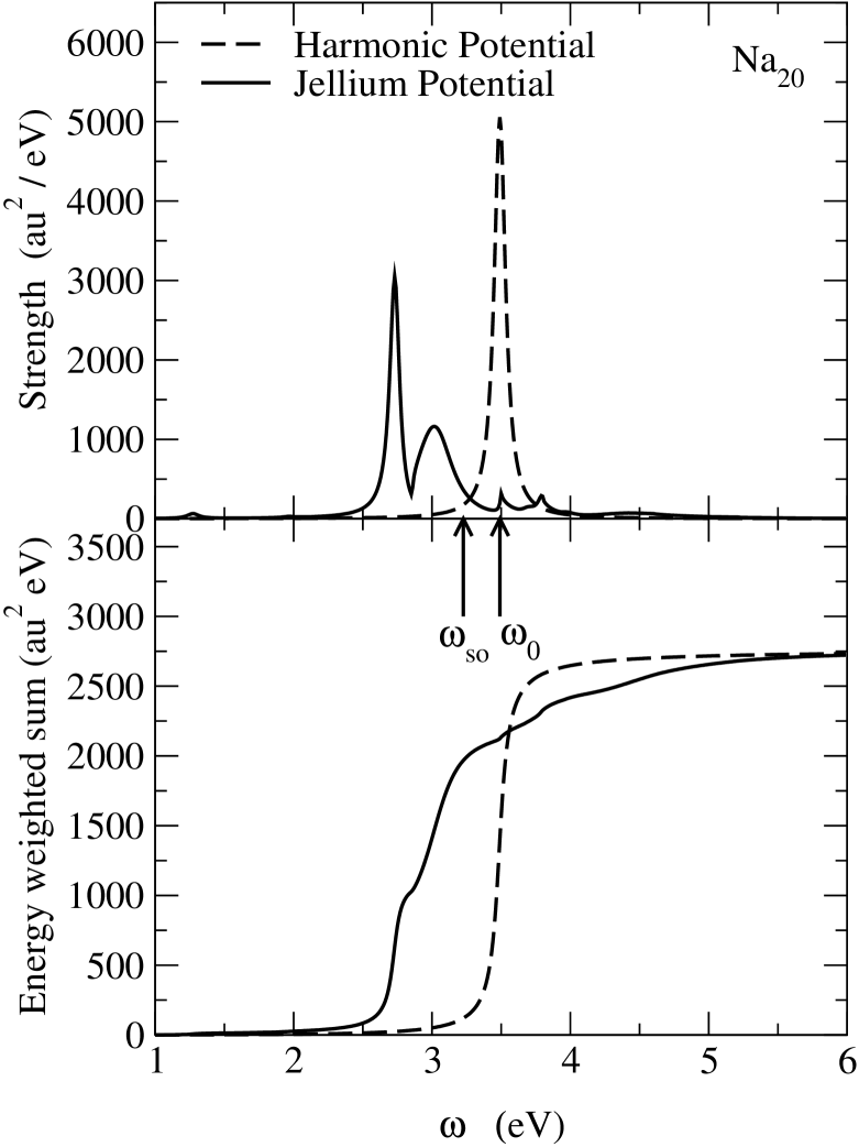
To assess the reliability of the variational shifts, we have numerically solved the RPA equations for the jellium model, using the computer program JellyRpa [13]. A typical spectrum is shown in Fig. 1. This represents Na₂₀ as a system of 20 electrons in a background spherical charge distribution with a density corresponding to $r_{s}=3.93$ a.u. and total charge $Q=20$. The strength function includes an artificial width of $\Gamma=0.1$ eV for display purposes. The Mie frequency, Eq. (1), is indicated by $\omega_{0}$, while the prediction of the spill-out formula, Eq.(3), is shown as $\omega_{so}$ in the figure. One sees that the strength function is fragmented into two large components that are considerably red-shifted from the Mie frequency, and smaller contributions at higher frequencies. The corresponding spectrum with the jellium background potential replaced by a pure harmonic potential is shown by the dashed line. The numerical RPA frequency agrees very well with the Mie value in this case, showing that the numerical algorithms used in JellyRpa are sufficiently accurate for our purposes. The red shift can be more easily displayed by a plot of the integrated strength function, shown in the lower panel of the figure. If we define the shift as the point where the integrated strength reaches half of the maximum value, it corresponds to $\delta\omega=0.166\,\omega_{\rm Mie}$. On the other hand, the collective formula for the red shift, Eq. (3), only gives $\delta\omega=0.058\,\omega_{\rm Mie}$, when the integral for $\Delta N$ is evaluated with the ground state density.

The strength becomes increasingly fragmented in heavier clusters, making a precise definition of the red shift problematic. We therefore have simplified the jellium model in our numerical computations to see the effects of the shift without the fragmentation of the strength that occurs physically. To this end we put all the electrons in the lowest $s$-orbital, treating them as bosons. Otherwise, the model is the same as the usual jellium model, with the electron orbitals determined self-consistently in a background charge density of a uniform sphere. This model is easily implemented with JellyRpa by assigning the occupation probabilities of the orbitals appropriately. Taking the density parameter as $r_{s}=3.93$ a.u., appropriate for sodium clusters, one finds that the ionization potential is rather close to the value of the usual (fermionic) jellium model. For example, in the cluster with $N=20$ atoms, the ionization potential $\epsilon$ has a value 2.84 eV for usual jellium model and the value 4.11 eV for our simplified $s$-wave treatment.

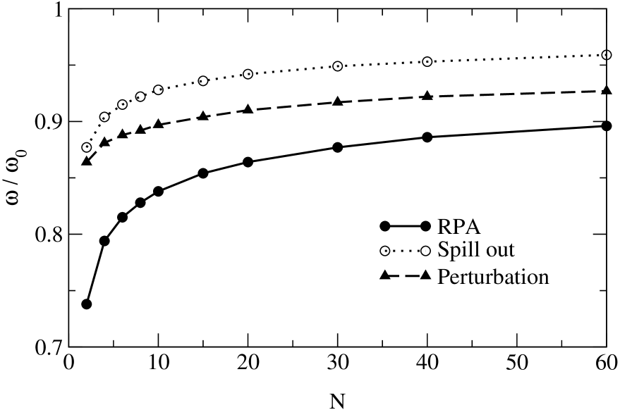
The results of the numerical calculation with the full effect of the surface are shown in Fig. 2 as the solid line. The collective spill-out correction from Eq. (3) is also shown as the dotted line. One sees that the additional shift due to the wave function perturbation is comparable to the spill-out correction, and has a similar $N$-dependence. The shift given by the variational formula Eq. (9) is shown by the dashed line. The functional dependence predicted by the formula is confirmed by the numerical calculations, but the coefficient of $N$ is too small by a factor of two or so.

VI Concluding remarks

We have developed a variational approach to treat perturbations to the collective RPA wave functions, and have applied it to the surface plasmon in small metal clusters. Our zeroth order solution is the same as that used by Gerchikov et al. [14] and Kurasawa et al. [15]. It corresponds to the center of mass motion, and is the exact RPA solution when the ionic background potential is a harmonic oscillator. The deviation of the background potential from the harmonic shape is responsible for the perturbation. The first order perturbation yields the well-known spill-out formula for the plasmon frequency, as was also shown in Refs. [14, 15]. The higher order corrections lead to the additional energy shift of the frequency [14], the anharmonicity of the spectrum [14], and the fragmentation of the strength [15]. Those effects were studied in Refs. [14, 15] by considering explicitly the couplings between the center of mass and the intrinsic motions. In this paper, we assumed some analytic form for the perturbation and determined its coefficient variationally. We found that this approach qualitatively accounts for the red shift of the collective frequency, but its magnitude came out too small by about a factor of two.

In order to have a more quantitative result, one would have to improve the variational wave function. An obvious way is to introduce more than one term. Our method may be viewed as the first iteration of any iterative method for RPA [21, 22, 23]. One may need more than one iteration to get a convergence and thus a sufficiently large energy shift. Another possible way is to construct the perturbed wave function based on the local RPA. The authors of Ref. [24] expanded the collective operator with local functions and solved a secular equation to determine the frequency. They showed that the expansion of the collective operator with three functions, $r\cos\theta,r^{3}\cos\theta$, and $r^{5}\cos\theta$, gives a satisfactory result for the collective frequency.

The method developed in this paper is general, and is not restricted to the surface plasmon in micro clusters. One interesting application may be to the giant dipole resonance in atomic nuclei. In heavy nuclei, the mass dependence of the isovector dipole frequency deviates from the prediction of the Goldhaber-Teller model, that is based on a simple c.m. motion[25, 26]. The shift of collective frequency can be attributed to the effect of deviation of the mean-field potential from the harmonic oscillator, and a similar treatment as the present one is possible.

REFERENCES

- [1] U. Kreibig and M. Vollmer, Optical Properties in Metal Clusters (Springer-Verlag, Berlin, 1995).
- [2] G.F. Bertsch and R. A. Broglia, Oscillations in Finite Quantum Systems (Cambridge University Press, Cambridge, 1994).
- [3] W.D. Knight, Z. Phys. D 12, 315 (1989)
- [4] K. Selby et al, Phys. Rev. B 43, 4565 (1991)
- [5] C. Bréchignac et al, Chem. Phys. Lett. 164, 433 (1989)
- [6] M. Schmidt and H. Haberland, Eur. Phys. J.D 6, 109 (1999)
- [7] T. Reiners, C. Ellert, M. Schmidt, and H. Haberland, Phys. Rev. Lett. 74, 1558 (1995).
- [8] W. Ekardt, Phys. Rev. B 32, 1961 (1985)
- [9] C. Yannouleas and R.A. Broglia, Phys. Rev. A 44, 5793 (1991)
- [10] K. Yabana and G.F. Bertsch, Phys. Rev. B 54, 4484 (1996)
- [11] C. Guet and W.R. Johnson, Phys. Rev. B 45, 11 283 (1992).
- [12] M. Madjet, C. Guet and W.R. Johnson, Phys. Rev. A 51, 1327 (1995).
- [13] G.F. Bertsch,“An RPA program for jellium spheres”, Computer Physics Communications, 60 (1990) 247.
- [14] L.G. Gerchikov, C. Guet, and A.N. Ipatov, Phys. Rev. A 66, 053202 (2002).
- [15] H. Kurasawa, K. Yabana and T. Suzuki, Phys. Rev. B 56, R10063 (1997).
- [16] W. Kohn, Phys. Rev. 123, 1242 (1961).
- [17] J.F. Dobson, Phys. Rev. Lett. 73, 2244 (1994).
- [18] G. Vignale, Phys. Rev. Lett. 74, 3233 (1995).
- [19] G. Vignale, Phys. Lett. A209, 206 (1995).
- [20] A. Minguzzi, Phys. Rev. A64 033604 (2001).
- [21] C.W. Johnson, G.F. Bertsch, and W.D. Hazelton, Comp. Phys. Comm. 120, 155 (1999).
- [22] A. Muta, J.-I. Iwata, Y. Hashimoto, and K. Yabana, Prog. Theo. Phys. 108, 1065 (2002).
- [23] H. Imagawa and Y. Hashimoto, Phys. Rev. C67, 037302 (2003).
- [24] P.G. Reinhard, M. Brack and O. Genzken, Phys. Rev. A41, 5568 (1990).
- [25] G. Bertsch and K. Stricker, Phys. Rev. C13, 1312 (1976).
- [26] W.D. Myers, W.J. Swiatecki, T. Kodama, L.J. El-Jaick, and E.R. Hilf, Phys. Rev. C15, 2032 (1977).