Compressibility Consideration in the Boundary of a Strongly Collapsing Bubble

Abstract

Equations of radial motion of a gas bubble in a compressible viscous liquid have been modified to account for compressibility at the bubble boundary. A new bubble boundary equation has been derived, including a new term resulted from liquid compressibility. The influence of this term has been numerically investigated using isothermal-adiabatic model for the gas inside the bubble. The results clearly indicate that, at the end of the collapse, the new term has a very significant role and its consideration dramatically changes the bubble characteristics. Moreover, the more intense the collapse is, the more significant the effect of the new term is. Also, it has been reasoned out that, the influence of the new term will be established even when the effects of mass (water vapor) exchange, chemical reactions, and gas dynamics inside the bubble are taken into account.

I Introduction

The problem of non-linear radial oscillations of a gas bubble in a liquid, when it experiences a high amplitude spherical sound field, is an old challenging problem. Several complications are present in this problem arising from the effects of heat conduction, mass diffusion, compressibility, chemical reactions, surface tension, and viscosity. Many authors have studied different aspects of this matter, but a rather complete description has not been presented yet.

The radial dynamics of a bubble in an incompressible liquid is described by the well-known incompressible Rayleigh-Plesset equation Rayleigh:1917 ; Noltingk:1951 . The extension of this equation to the bubble motion in a compressible liquid has been studied by many authors; for example Herring Herring:1941 , Trilling Trilling:1952 , Gilmore Gilmore:1952 , Keller and Kolodner Keller:1956 , Flynn Flynn:1975 , Lastman and Wentzell Lastman:1979 , Löfstedt et al. fstedt:1993 , and Nigmatulin et al. Nigmatulin:2000 . In these works, several different forms of the compressible bubble dynamics equations have been presented, using different approximation for consideration of the compressibility effects. On the other hand, the influences of heat conduction and mass diffusion in the bubble motion have been reported by Hickling Hickling:1963 , Fujikawa and Akumatsu Fujikawa:1980 , and Yasui Yasui:1997 .

In a generalized approach, Prosperetti and Lezzi Prosperetti:1987 used a singular-perturbation method of the bubble-wall Mach number and derived a one-parameter family of equations describing the bubble motion in the first order approximation of compressibility. This family of equations are written as:

$$\left({1-(\eta+1)\frac{\dot{R}}{C}}\right)\!R\ddot{R}+\frac{3}{2}\left({1-\frac{1}{3}(3\eta+1)\frac{\dot{R}}{C}}\right)\!\dot{R}^{2}=$$

$${\frac{R}{\rho C}\frac{d}{dt}\left({P_{l}-P_{a}}\right)\!+\!\left({1+(1-\eta)\frac{\dot{R}}{C}}\ \right)\!\!\!\left(\frac{P_{l}-P_{a}-P_{0}}{\rho}\right)},$$

where, $R$, $C$, $P_{0}$, $P_{a}$, and $\rho$ are bubble radius, liquid sound speed, ambient pressure, driving pressure, and density of the liquid, respectively. Also, $\eta$ is an arbitrary parameter. Equation (I) must be supplemented by a boundary condition equation at the bubble interface to relate the liquid pressure, $P_{l}$, to the gas pressure inside the bubble. Like all previous authors, Prosperetti and Lezzi Prosperetti:1987 used the following incompressible equation for this purpose:

$$P_{l}=P_{g}-4\mu\frac{\dot{R}}{R}-\frac{2\sigma}{R},$$ (2)

where, $P_{g}$, $\mu$, and $\sigma$ are gas pressure at the bubble interface, liquid first viscosity coefficient, and surface tension, respectively. As Prosperetti and Lezzi showed Prosperetti:1987 , different existing forms of the bubble dynamics equations belong to this single parameter family of equations, corresponding to different values of $\eta$. Especially, $\eta=1$ and $\eta=0$ correspond to Keller and Miksis equation Keller:1980 and Herring-Trilling equation Herring:1941 ; Trilling:1952 , respectively.

Two specific approximations have been considered in the derivation of Eq’ns. (I) and (2). First, Eq’n. (I) has been derived from the Euler equation, in which the liquid viscosity effects have been neglected. However, these effects are not important in the usual applications of the bubble dynamics equations. It can be shown Moshaii:2002 that these effects are significant when $\mu\gtrsim\rho CR_{0}$, where $R_{0}$ is the bubble ambient radius. Therefore, for micron size and larger bubbles the elimination of these effects is thoroughly justified.

The second approximation, which is more important, is the incompressibility assumption of the liquid and the gas at the bubble interface, which has been used in the derivation of Eq’n. (2). Note that, all of the effects of the liquid compressibility in the work of Prosperetti and Lezzi, as well as in all previous works, have been resulted from the liquid motion around the bubble, but not from the bubble boundary condition equation. In fact, all previous authors, on one hand take into account the compressibility of the liquid motion around the bubble, but on the other hand neglect its consideration at the bubble interface. Although Eq’n. (2) has widely been used in all old and recent works Rayleigh:1917 ; Noltingk:1951 ; Herring:1941 ; Trilling:1952 ; Gilmore:1952 ; Keller:1956 ; Flynn:1975 ; Lastman:1979 ; fstedt:1993 ; Nigmatulin:2000 ; Hickling:1963 ; Fujikawa:1980 ; Yasui:1997 ; Prosperetti:1987 ; Keller:1980 , but its applicability for the bubble motion needs to be clarified (especially at the end of the collapse, where the bubble motion is significantly compressible).

In this paper, we have modified Eq’n. (2) considering the effects of compressibility at the bubble interface for both the liquid and the gas. The modified equation has new terms resulted from the effects of two coefficients of viscosity of the liquid and the gas. This work shows that the liquid compressibility effects in the bubble dynamics originate from two sources. First, they originate from the liquid motion around the bubble, which has already been presented in the generalized Eq’n. (I). Second, they are initiated through the liquid compressibility consideration at the bubble interface as presented in this work. We have performed numerical analysis to investigate the influence of the modification of Eq’n. (2).

II Compressible Bubble Boundary Equation

To derive the compressible bubble boundary equation, we assume that, the motions of the bubble interface and the surrounding liquid are always spherically symmetric. The continuity equation and the radial component of the stress tensor can be written as:

$$\frac{1}{\rho}\left[{\frac{\partial\rho}{\partial t}+u\frac{\partial\rho}{\partial r}}\right]=-\frac{\partial u}{\partial r}-\frac{2u}{r}=-\Delta,$$ (3)

$$T_{rr}=-p+\lambda\Delta+2\mu\left(\frac{\partial u}{\partial r}\right).$$ (4)

where, $\rho$, $u$, $p$, and $\Delta$ are density, velocity, pressure, and divergence of the velocity, respectively. Also, $\lambda$ is the second coefficient of viscosity. Inserting $\partial u/\partial r$ from Eq’n. (3), into Eq’n. (4) yields:

$$T_{rr} = -p+(\lambda+2\mu)\left(\frac{\partial u}{\partial r}+\frac{2u}{r}\right)-4\frac{\mu u}{r}$$ (5)

$$= -p+(\lambda+2\mu)\triangle-4\frac{\mu u}{r}.$$

The velocity divergence, $\triangle$, can be written as:

$$\triangle=-\frac{1}{\rho}\frac{d\rho}{dt}=-\frac{1}{\rho c^{2}}\frac{dp}{dt},$$ (6)

where, the sound speed, $c$, is defined as $c^{2}=dp/d\rho$. The boundary continuity requirement at the bubble interface is:

$$T_{rr}(liquid)\mid_{R}=T_{rr}\left(gas\right)\mid_{R}+2\frac{\sigma}{R}.$$ (7)

Applying Eq’n. (5) for the gas and the liquid parts of Eq’n. (7) leads to:

$$P_{l}+4\frac{\mu\dot{R}}{R} - \left(\lambda+2\mu\right)\triangle_{l}=P_{g}+4\frac{\mu_{g}\dot{R}}{R}$$ (8)

$$- \left(\lambda_{g}+2\mu_{g}\right)\triangle_{g}-2\frac{\sigma}{R},$$

where, $\mu_{g}$ and $\lambda_{g}$ are the first and the second coefficients of viscosity of the gas at the bubble interface, respectively. Also, $\Delta_{l}$ and $\Delta_{g}$ are the divergence of velocity of the liquid and the gas, respectively. Substituting the divergence of velocity for the liquid and the gas from Eq’n (6) into Eq’n. (8) yields:

$$P_{l}+4\frac{\mu\dot{R}}{R} + \left(\frac{\lambda+2\mu}{\rho C^{2}}\frac{dP_{l}}{dt}\right)=P_{g}+4\frac{\mu_{g}\dot{R}}{R}$$ (9)

$$+ \left(\frac{\lambda_{g}+2\mu_{g}}{\rho_{g}}\frac{d\rho_{g}}{dt}\right)-2\frac{\sigma}{R},$$

where $\rho_{g}$ is the gas density at the bubble interface. Equation (9) represents the bubble boundary equation containing all effects of the compressibility and the viscosity of both the liquid and the gas. Comparison of Eq’ns. (2) and (9) indicates the existence of three new terms in Eq’n. (9) due to the liquid and the gas compressibility and viscosity effects. Here, we concentrate on the effects of the new term arising from the liquid compressibility. Therefore, the gas viscosity effects are neglected due to their smallness relative to the liquid viscosity as in previous works Rayleigh:1917 ; Noltingk:1951 ; Herring:1941 ; Trilling:1952 ; Gilmore:1952 ; Keller:1956 ; Flynn:1975 ; Lastman:1979 ; fstedt:1993 ; Nigmatulin:2000 ; Hickling:1963 ; Fujikawa:1980 ; Yasui:1997 ; Prosperetti:1987 ; Keller:1980 . Under this circumstance, Eq’n. (9) becomes:

$$P_{l}+\left(\frac{\lambda+2\mu}{\rho C^{2}}\frac{dP_{l}}{dt}\right)=P_{g}-4\frac{\mu\dot{R}}{R}-2\frac{\sigma}{R}.$$ (10)

To generalize the argument, we express Eq’ns. (I) and (10) in dimensionless forms. The dimensionless variables are:

$$R^{\ast}=\frac{R}{R_{0}}, \dot{R^{\ast}}=\frac{\dot{R}}{C},\;\;\;\;t^{\ast}=\frac{tC}{R_{0}},\;\;\;\;P_{l}^{\ast}=\frac{P_{l}}{\rho C^{2}},\;\;\;\;$$ (11)

$$P_{g}^{\ast}=\frac{P_{g}}{\rho C^{2}},\;\;\;\;P_{a}^{\ast}=\frac{P_{a}}{\rho C^{2}},\;\;\;\;$$

where, $R_{0}$ is the ambient radius of the bubble. Substituting the dimensionless variables into Eq’ns. (I) and (10) results the dimensionless equations:

$$\left(1-(\eta+1)\dot{R}^{\ast}\right)\!\!\! \!\!\!\!\!\!R^{\ast}\ddot{R^{\ast}}+\frac{3}{2}\left(1-\frac{1}{3}(3\eta+1)\dot{R}^{\ast}\right)\dot{R}^{\ast 2}$$ (12)

$$= \!\left(\!{1+(1-\eta)\dot{R}^{\ast}}\!\right)\!\!\left(P_{l}^{\ast}-P_{a}^{\ast}-P_{0}^{\ast}\right)$$

$$+ R^{\ast}\frac{d}{dt^{\ast}}\!\left(P_{l}^{\ast}-P_{a}^{\ast}\right),$$

$$P_{l}^{\ast}=P_{g}^{\ast}-4\frac{\mu^{\ast}\dot{R}^{\ast}}{R^{\ast}}-2\frac{\sigma^{\ast}}{R^{\ast}}-\left(\lambda^{\ast}+2\mu^{\ast}\right)\frac{dP_{l}^{\ast}}{dt^{\ast}}.$$ (13)

The quantities $\sigma^{\ast}$, $\lambda^{\ast}$, and $\mu^{\ast}$ are the dimensionless form of surface tension, first, and second viscosity coefficients of the liquid and are defined as: $\sigma^{\ast}=\sigma/\rho R_{0}C^{2}$, $\lambda^{\ast}=\lambda/\rho R_{0}C$, and $\mu^{\ast}=\mu/\rho R_{0}C$, respectively. These dimensionless quantities are basically the inverse of Weber Number and Reynolds Number.

It should be mentioned that, although the effects of compressibility in Eq’n. (12) are in the first order approximation, but these effects have been introduced completely in Eq’n. (13). To quantify the effects of our modification, we have performed our calculations within the framework of Eq’n. (12), using $\eta=1$. Of course, similar results are obtained using the other values of $\eta$ in Eq’n. (12), because of the similarity of the order of approximation in all equations corresponding to different values of $\eta$.

III Numerical Analysis

To quantify the effects of the new term in Eq’n. (13), numerical analysis was carried out for the conditions of Single Bubble Sonoluminescence (SBSL) Brenner:2002 ; Barber:1997 . The driving pressure in its dimensionless form was $P_{a}^{\ast}(t)=-P_{a}^{\ast}\sin\left(\omega^{\ast}t^{\ast}\right)$, where $\omega^{\ast}$ is dimensionless angular frequency and is defined as $\omega R_{0}/C$. To have a well-posed problem, the value of the gas pressure at the bubble interface, $P_{g}^{\ast}$, must be specified. It can be determined, in the most complete approach, from the numerical solution of the conservation equations for the bubble interior along with Eq’ns. (12) and (13) simultaneously. Also, the bubble content changes during the bubble evolution because of the chemical reactions at the end of the collapse. In addition, the mass exchange and the heat transfer between the bubble and the surrounding liquid affect the bubble interior.

During the past ten years, several different approaches have been presented to describe the real state of the gas and its evolution considering the above-mentioned complexities. These approaches, which at first assumed inviscid and without consideration of chemical reactions, heat transfer, and mass exchange C.C.WU ; Moss:1994 , became gradually more complex by including dissipating effects of radiative transfer Kondict:1995 , heat transfer, and viscous gas dynamics Voung:1996 ; Yuan:1998 . Recent gas dynamic model of Storey and Szeri Storey:2000 accounts for all effects of chemical reactions and water vapor evaporation and condensation.

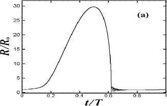
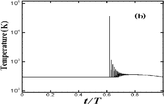
Figure 1: Time variations of the bubble characteristics; (a) radius, (b) gas temperature for the compressible boundary condition in one period of the applied pressure field.

During the bubble motion, strong spatial inhomogeneities inside the bubble are not remarkably revealed unless at the end of the collapse. Therefore, the uniformity assumption for the bubble interior seems to be useful and provides many features of the bubble motion Barber:1997 ; Brenner:2002 . By this assumption, the gas pressure inside the bubble is obtained assuming polytropic evolution for the gas bubble as:

$$P_{g}^{\ast}=\left(P_{0}^{\ast}+2\sigma^{\ast}\right)\left(\frac{1-a^{\ast 3}}{R^{\ast 3}-a^{\ast 3}}\right)^{\gamma},$$ (14)

where, Van der Waals equation of state has been used. Here, $a^{\ast}$ is the dimensionless Van der Waals hard core radius; $a^{\ast}=a/R_{0}$. The bubble evolution is assumed to be isothermal ($\gamma=1.0$) for the radii larger than $R_{0}$, when the bubble moves relatively slow. While, adiabatic assumption ($\gamma=\Gamma$, where $\Gamma$ is the ratio of the specific heats of the bubble interior) is applied for the smaller radii, when the bubble experiences rapid changes Barber:1997 .

Hilgenfeldt et al. Hilgenfeldt:1999 extended this model considering $\gamma$ to be a function of the Peclet number of the bubble. Of course, the Peclet number changes with the variations of the bubble radius and the bubble velocity. They showed that, many features of SBSL can be explained by their model. However, in practice there is very small difference (less than 5%) between the Hilgenfeldt et al.’s model and the isothermal-adiabatic model Putterman:2001 . Although, these two models can not illustrate production of discontinuities and shock waves at the end of the collapse, but they are really useful for our purpose to investigate the importance of the new term during the collapse. It should be mentioned that, these models have been used in several recent works in sonoluminescence studies ISO-ADI-model .

We have used isothermal-adiabatic model in this paper. Also, we have argued about the extension of the results for more complicated models. Under these circumstances, the time variations of the bubble properties under the framework of Eq’n (12) (for $\eta=1$) have been numerically calculated for two cases: (a) compressible boundary condition (Eq’n. 13) and (b) incompressible boundary condition (Eq’n. 2). We used Runge-Kutta method for our numerical analysis. The constants and the parameters used in the calculations were set for an air bubble in water at room temperature, $T_{0}=293.0~{}K$, and atmosphere pressure, $P_{0}=1.0~{}atm$, CRC:1991 ; $\rho=998.0~{}kg/m^{3}$, $C=1483.0~{}m/s$, $\mu=1.01\times 10^{-3}~{}kg/ms$, $a^{\ast}=1.0/8.745$, $\sigma=0.0728~{}kgs^{-2}$, and $\Gamma=1.4$. The second coefficient of viscosity of water was set to be $\lambda=2.23~{}\mu$. It was derived from the value of the bulk viscosity of water at room temperature that, $\mu_{b}=\lambda+(2\mu/3)=2.9\mu$ Pierce:1991 . Also, the angular frequency of the deriving pressure was $\omega=2\pi\times 26.5~{}kHz$.

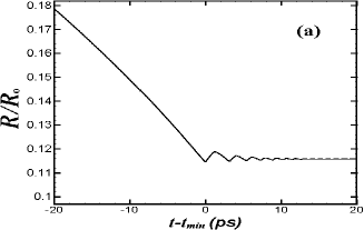
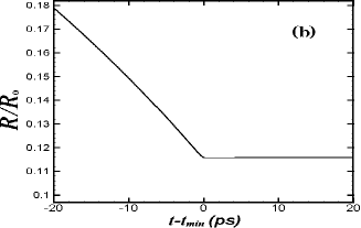
Figure 2: Time variations of the bubble radius according to (a) compressible and (b) incompressible cases. The time interval of this figures is 40 ps around the minimum radius time $(t_{min})$.

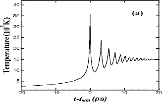
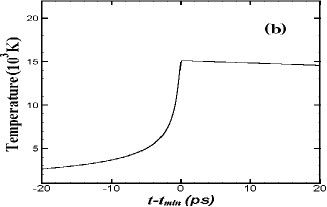
Figure 3: Time variations of the gas temperature when the bubble reaches its minimum radius according to (a) compressible and (b) incompressible cases.

IV Results

The results of our calculations have been illustrated in Figs. (1-5) for $P_{a}=1.6~{}atm$ and $R_{0}=2.0~{}\mu m$. Similar values for these parameters were reported in the results of recent experimental works of Ketterling and Apfel Ketterling:2000 , Simon et al. Simon:2001 , and Vazquez et al. Vazquez:2002 . Figure (1) shows the variations of the bubble radius and the gas temperature in one period of the applied pressure field using the compressible boundary condition. The bubble motion has incompressible characteristics during a period, except for an infinitesimal time interval at the end of the collapse. Basically, the new term in Eq’n. (13) originates from the compressibility of the liquid motion. Therefore, it is expected that, its effects not to be revealed, until the bubble motion becomes significantly compressible. The results of our calculations clearly confirm this point. Except for the end of the collapse, the differences between the bubble characteristics resulting from the compressible and incompressible boundary conditions are less than $1.0\%$. This result thoroughly justifies the elimination of the new viscous term in Eq’n. (13) for all times, but not for the end of the collapse. Indeed, in Fig. (1), the results for the bubble properties of the two boundary conditions completely coincide. However, the maximum bubble temperature in Fig. 1(b) has a considerable increase relative to that of the incompressible case. This discrepancy instigated us for further concentration of the bubble properties around the minimum bubble radius.

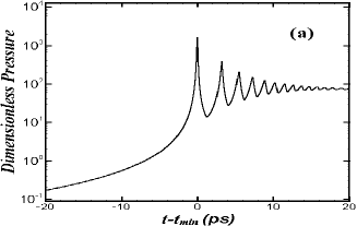
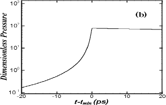
Figure 4: Time variations of the dimensionless gas pressure ($P_{g}/\rho C^{2}$) around the time of minimum radius according to (a) compressible and (b) incompressible boundary conditions.

In Figs. (2-4), we have presented the evolution of the bubble characteristics using compressible boundary condition (a), and incompressible boundary condition (b), around the minimum radius time. The time interval of these figures is 40 ps. Since, the bubble experiences its maximum compression at the end of the collapse, the effects of the new term in Eq’n. (13) are more significant during this time interval.

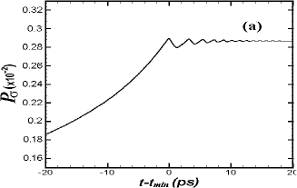
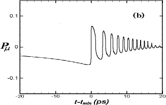
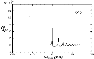
Figure 5: Time variations of three dimensionless pressure terms in equation (13) namely; (a) surface tension term: $P_{\sigma}=2\sigma^{\ast}/R^{\ast}$, (b) damping viscous term: $P_{\mu}=4\mu^{\ast}\dot{R}^{\ast}/R^{\ast}$, and (c) new viscous term: $P_{\lambda\mu}=(\lambda^{\ast}+2\mu^{\ast})(dP_{l}^{\ast}/dt^{\ast})$, when the bubble reaches its minimum radius.

Figure (2) shows the bubble radius evolution for the two boundary conditions. This figure illustrates a considerable difference between the compressible and incompressible cases. After the bubble reaches its minimum radius, a number of small bouncing oscillations appear in the graph of the compressible case, which do not occur in that of the incompressible case. The period of these oscillations is nearly 3 ps. The details of our calculations show that, the times of minimum radius for the two cases are the same. While, the minimum radius for the new Eq’n. (13) is 1% less than that of the old Eq’n. (2).

Figure (3) represents the time variations of the gas temperature near the minimum radius time. It evidently represents that, introducing the new viscous term in Eq’n. (13) strongly affects the gas temperature evolution at the end of the collapse. After the minimum radius time, the incompressible case illustrates smooth behavior for the bubble temperature. While, remarkable sharp peaks appear in the temperature evolution using the compressible boundary condition. Also, as the bubble goes away from the minimum radius, the peaks become weaker. Note that, the value of the maximum temperature increases considerably (nearly 2.4 times) for the new boundary equation.

Comparison of the gas pressure evolution for the two cases is shown in Fig. (4). Similar behaviors as in Fig. (3) are observed in this figure for the difference between the new and the old boundary equations. Note that, the gas pressure is much more sensitive to the presence of the new viscous term compared to the gas temperature. In fact, the presence of the new term increases the maximum pressure more than one order of magnitude.

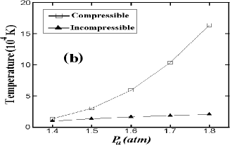
Figure 6: (a) The maximum dimensionless gas pressure versus different amplitudes of the pressure field according to the compressible (squares) and incompressible (filled triangles) cases. (b) The maximum gas temperature corresponding to the same data points of the case (a). The calculated points are for constant ambient radius $R_{0}=1.5~{}\mu m$. Other constants and parameters were set as Fig.1

In Fig. (5), the time variations of the three different pressure terms in Eq’n. (13) have been illustrated near the minimum radius. These terms are due to the effects of surface tension and viscosity, i.e. $P_{\sigma}=2\sigma^{\ast}/R^{\ast}$, $P_{\mu}=4\mu^{\ast}\dot{R}^{\ast}/R^{\ast}$, and $P_{\lambda\mu}=(\lambda^{\ast}+2\mu^{\ast})(dP_{l}^{\ast}/dt^{\ast})$. This figure clearly shows that, at the end of collapse, the collective effects of the viscous terms are by far greater than the surface tension term. Moreover, the new viscous term, $P_{\lambda\mu}$, is the dominant term in this time interval. Note that, the order of the maximum values of the three pressure terms are completely different. $P_{\lambda\mu}$ is the highest (up to $10^{3}$) and $P_{\sigma}$ is the lowest (less than $10^{-2}$). These results emphasize that, the elimination of $P_{\lambda\mu}$ is not reasonable, when the bubble evolves near the minimum radius.

Figures (6) and (7) illustrate the dependence of the peak pressure and the peak temperature of the bubble to the driving pressure and to the ambient radius, for the two boundary equations. Figure (6) is for the case in which, the ambient radius is constant ($R_{0}=1.5~{}\mu m$), while the amplitude of the driving pressure is increased from $P_{a}=1.4~{}atm$ to $1.8~{}atm$. On the other hand, Fig. (7) shows the results for the constant amplitude of the driving pressure, ($P_{a}=1.7~{}atm$), with varying $R_{0}$ from $1.0~{}\mu m$ to $5.0~{}\mu m$. Different values of $R_{0}$ can be experimentally adapted for a specific value of $P_{a}$, adjusting the concentration of the dissolved gas in the liquid Barber:1997 .

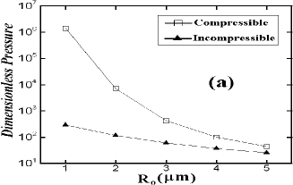
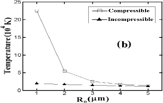
Figure 7: (a) The maximum dimensionless gas pressure versus different bubble ambient radii according to the compressible (squares) and incompressible (filled triangles) cases. (b) The maximum gas temperature corresponding to the same data points of the case (a). The calculated points are for constant driving pressure amplitude $P_{a}=1.7~{}atm$. Other constants and parameters were set as Fig.1

The dependence of the maximum pressure and the maximum temperature of the bubble to $P_{a}$ is represented in Fig. (6). There are significant differences between these bubble properties resulted from the new boundary condition with those of the old one. The differences are more considerable for the higher driving pressures. Moreover, the differences are more remarkable for the maximum pressure than the maximum temperature. Note that, for $P_{a}=1.8~{}atm$, the maximum temperature using the new equations is about 8 times greater than that of the old ones. While, the increase of the maximum pressure in this case is about 1400 times. These results indicate that, the compressibility effects should be much higher than what is considered in the incompressible case.

The effects of the variation of $R_{0}$ on the mentioned bubble properties are illustrated in Fig. (7). Similar considerable differences between the new and the old cases as in Fig. (6) are also present in this figure. The differences are more significant for the smaller ambient radii.

Time grid resolution study of the problem shows that, the values of the bubble properties at the end of collapse are sensitive to the step size. But, this sensitivity disappears as the resolution is reduced sufficiently. Figure (8), presents the step size dependence of the value of maximum gas pressure for the compressible case, where $P_{a}=1.8~{}atm$ and $R_{0}=1.5~{}\mu m$. It shows a diminishing step size dependence bellow $10^{-17}s$.

It should be mentioned that, although the results of the last figures were acquired by assumption that $\Gamma=1.4$ (the bubble content was assumed to be a diatomic gas), however the appearance of the new bubble behavior is independent of the selected value of $\Gamma$ (and gas content). Figure (9) shows the evolution of the bubble temperature for two different states; $\Gamma=1.67$ (monoatomic gas) and $\Gamma=1.33$ (polyatomic gas). The comparison of Figs. (3) and (9) shows that, the new bubble behavior will be established even when the gas content changes. Of course, as Figs. (3) and (9) indicates, the configuration and the number of the new peaks depend on the value of $\Gamma$. The number of peaks is more for the smaller $\Gamma$. While, the values of the peak temperatures are greater for higher $\Gamma$, due to the decrease of the number of the degrees of freedom.

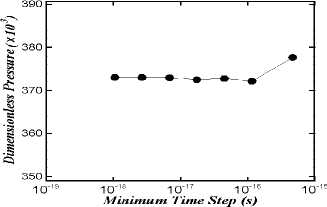
Figure 8: Time grid resolution dependence of the maximum gas pressure for the compressible case, where $P_{a}=1.8~{}atm$ and $R_{0}=1.5~{}\mu m$.

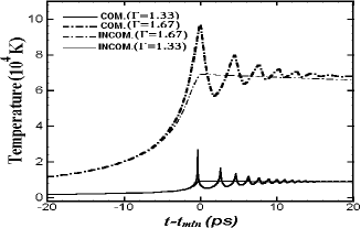
Figure 9: Dependence of the gas temperature evolution near the minimum radius to the value of $\Gamma$, according to compressible (thick) and incompressible (thin) cases. The dashed and solid curves are related to $\Gamma=1.33$ and $\Gamma=1.67$, respectively. Other constants and parameters are the same as Fig. 1. Note that $t_{min}$ for $\Gamma=1.33$ is nearly half picosecond less than that of $\Gamma=1.67$.

V Discussion

Although, the isothermal-adiabatic model used in this study does not account for the effects of gas dynamics, chemical reactions and water vapor exchange, but the consideration of these effects can not cover the importance of the new term at the end of the collapse. In this section, the influences of these corrections on the new bubble behavior are argued:

(i) Gas dynamics: Considerations of the gas dynamics effects inside the bubble have been presented by several different approaches C.C.WU ; Moss:1994 ; Kondict:1995 ; Voung:1996 ; Yuan:1998 . These approaches show that, the overall bubble temperature and pressure at the collapse in gas dynamics models are at least no less than those of the isothermal-adiabatic model. In fact, in the gas dynamics models the bubble experiences more compression. Therefore, the pressure upon the liquid will be greater in the gas dynamic models. This means that, the effects of the new viscous term should even be more remarkable in the gas dynamics models.

(ii) Chemical reactions: The temperature of the bubble at the end of the collapse is high enough (higher than 10000 K) to destroy the chemical bonds of N₂ and O₂ molecules of the air bubble. The chemical reactions between the water vapor and the existing oxygen and nitrogen atoms mainly produce very soluble substances in water (HN, NH3, and HNO3), which are completely absorbed. Therefore, a sonoluminescence air bubble mainly contains inert gases. This idea, which was initially presented by Lohse et al. Lohse:1997 is known as dissociation hypothesis (DH) and has been confirmed very well by experimental reports exp . The simulation of chemical reactions at the collapse in a gas dynamics model has been recently presented by Storey and Szeri Storey:2000 . Their work shows that, a considerable decrease appears in the bubble peak temperature due to the consideration of chemical reactions. Since most of the reactions at the collapse are endothermic, their influences can be considered as addition of some extra degrees of freedom Brenner:2002 . This means that, the bubble actually evolves near the minimum radius by an effective exponent, $\Gamma_{\!e\!f\!f\!}$, which is less than the monoatomic exponent ($\Gamma=5/3$). However, according to our results, the appearance of the new behaviors is independent of the values of $\Gamma$. Therefore, the new bubble behaviors should be established even when chemical reactions are introduced in the model.

(ii) Water vapor: Evaporation and condensation of the water vapor between the bubble and the liquid occur during the expansion and compression of the bubble. Recent simulations Yasui:1997 ; Storey:2000 ; Togel:2003 show that, a large amount of water vapor evaporates into the bubble during the expansion. Indeed, at maximum radius, about 90% of the bubble content is water vapor. During the collapse, the water vapor molecules condense to the liquid so that, near the minimum radius only a small fraction of a sonoluminescence bubble is water vapor and the remaining is mainly inert gases Yasui:1997 ; Storey:2000 ; Togel:2003 . Presence of these water vapor molecules inside the bubble decreases the maximum temperature due to the increase of the bubble’s total degrees of freedom. This effect causes more decrease of the effective exponent Brenner:2002 . Therefore, similar to our argument in the last paragraph, the effects of the water vapor can not also cover the strong effects of the compressibility consideration of this work.

VI Conclusions

The modification of the bubble dynamics equation to account for the viscosity of a compressible liquid was performed by deriving a new equation for the bubble boundary. This equation includes a new term, which has been resulted from simultaneous effects of viscosity and compressibility of the liquid. The new term is the prominent term at the end of the collapse, where the bubble is highly compressed. It exhibits its role by intensifying the strength of the collapse. The more intense the collapse is, the more significant the role of the new term is. Moreover, the new effects can not completely be covered by the dissipating effects of the water vapor and the chemical reactions.

The results of this work strongly indicate that, the neglect of the new term at the end of the collapse in the previously derived equations is not reasonable. Especially, it is more remarkable for high amplitudes single bubble sonoluminescecne. It is expected that, these new theoretical results can be confirmed in the experiments, if resolution of the bubble motion measurement at the end of an intense collapse is less than 0.1 ns. Of course, a stable high amplitude sonoluminescence bubble can be produced, if the concentration of the dissolved gas in the liquid is sufficiently small Simon:2001 .

References

- (1) L. Rayleigh, Philos. Mag., 34, 94 (1917); M. S. Plesset, J. Appl. Mech. 16, 277 (1949).
- (2) B. E. Noltingk and E. A. Neppiras, Proc. Phys. Soc. London B 63, 674 (1950); B. E. Noltingk and E. A. Neppiras, Proc. Phys. Soc. London B 64, 1032 (1951); H. Poritsky, Proc. First U. S. National Congress on Applied Mechanics, New York, 813, (1952), edited by E. Sternberg.
- (3) C. Herring, OSRD Rep. No. 236 (NDRC C4-sr-10-010) (1941).
- (4) L. Trilling, J. Appl. Phys. 23, 14 (1952).
- (5) F. R. Gilmore, Rep. No. 26-4, Hydrodyn. Lab., Calif. Inst. Tech. (1952).
- (6) J. B. Keller and I. I. Kolodner, J. Appl. Phys. 27, 1152 (1956).
- (7) H. G. Flynn, J. Acoust. Soc. Am. 57, 1379 (1975).
- (8) G. J. Lastman and R. A. Wentzell, Phys. Fluids 22, 2259 (1979); G. J. Lastman and R. A. Wentzell, J. Acoust. Soc. Am. 69, 638 (1981) .
- (9) R. Löfstedt, B. P. Barber, and S. J. Putterman, Phys. Fluid A 5, 2911 (1993).
- (10) R. I. Nigmatulin, I. SH. Akhatov, N. K. Vakhitova, and R. T. Lahey, J. Fluid Mech. 414, 47 (2000).
- (11) R. Hickling, J. Acoust. Soc. Am. 35, 967 (1963).
- (12) S. Fujikawa and T. Akamatsu, J. Fluid Mech. 97, 481 (1980).
- (13) K. Yasui, Phys. Rev. E 56, 6750 (1997).
- (14) (a) A. Prosperetti and A. Lezzi, J. Fluid Mech. 168, 457 (1986); (b) A Lezzi and A. Prosperetti, J. Fluid Mech. 185, 289 (1987).
- (15) J. B. Keller and M. Miksis, J. Acoust. Soc. Am. 68, 628 (1980).
- (16) A. Moshaii, M. Taeibi-Rahni, R. Sadighi, and H. Massah, Proceeding of the Ninth Asian Congress of Fluid Mechanics, Isfahan, 96, (2002), edited by E Shirani and A. Pishevar I.U.T. Publication Center, Isfahan, Iran.
- (17) B. P. Barber, R. A. Hiller, R. Löfstedt, S. J. Putterman, and K. R. Weninger, Phys. Rep. 281, 65 (1997).
- (18) M. P. Brenner, S. Hilgenfeldt, and D. Lohse, Rev. Mod. Phys.74, 425 (2002).
- (19) C. C. Wu and P. H. Roberts, Phys. Rev. Lett. 70, 3424 (1993).
- (20) W. C. Moss, D. B. Clarke, J. W. White, and D. A. Young, Phys. Fluids 6, 2979 (1994); W. C. Moss, D. B. Clark, and D. A. Young, Scince, 276, 1398 (1997).
- (21) L. Kondic, J. I. Gersten, and C. Yuan, Phys. Rev. E 52, 4976 (1995).
- (22) V. Q. Voung and A. J. Szeri, Phys. Fluids 8, 2354 (1996).
- (23) L. Yuan, H. Y. Cheng, M.-C. Chu, and P. T. Leung, Phys. Rev. E 57, 4265 (1998).
- (24) B. D. Storey and A. J. Szeri, Proc. Roy. Soc. London, Ser. A 456, 1685 (2000); B. D. Storey and A. J. Szeri, Proc. Roy. Soc. London, Ser. A 457, 1685 (2001).
- (25) S. Hilgenfeldt, S. Grossmann, and D. Lohse, Phy. Fluids 11, 1318 (1999); S. Hilgenfeldt, S. Grossmann, and D. Lohse, Nature (London). 398, 402 (1999).
- (26) S. J. Putterman, P. G. Evans, G. Vazquez, Nature (London). 409, 782 (2001); The authors also compare numerical results of the two models for the same conditions as Fig. 2 of Ref. 25(a). In fact, less than 5% difference between the two models exists.
- (27) I. Akatov, et al., Phys. Rev. E 55, 3747, (1997); D. Hammer and L. Formmhold, Phys. Rev. E 85, 1326 (2000); L. Yuan, C. Y. Ho, M. C. Cho, and P. T. Leung, Phys. Rev. E 64, 016317 (2001).
- (28) CRC Handbooh of Chemistry and Physics, edited by D. Lide, CRC Press, Boca Raton, FL, (1991)
- (29) A. D. Pierce, Acoutics - An Introduction to Its Physical Principles and Applications (Acoustical Society of America, New York, 1991).
- (30) J. A. Ketterling and R. E. Apfel, Phys. Rev. E 61, 3832 (2000).
- (31) G. Simon, I. Csabai, A. Horvath, and F. Szalai, Phys. Rev. E 63, 026301 (2001).
- (32) G. Vazquez, C. Camara, S. J. Putterman, and K. Weninger, Phys. Rev. Lett. 88, 197402(2002).
- (33) D. Lohse, M. P. Brenner, T. Dupont, S. Hilgenfeldt, and B. Johnston, Phys. Rev. Lett. 78, 1359 (1997); D. Lohse, S. Hilgenfeldt, J. Chem. Phys. 107, 6986 (1997).
- (34) T. J. Matula and L. A. Crum, Phys. Rev. Lett. 80, 865 (1998); J. A. Ketterling and R. E. Apfel, Phys. Rev. Lett. 81, 4991 (1998).
- (35) R. Toegel, D. Lohse, J. Chem. Phys. 118, 1863 (2003).