Sensor Alignment by Tracks

Abstract

Good geometrical calibration is essential in the use of high resolution detectors. The individual sensors in the detector have to be calibrated with an accuracy better than the intrinsic resolution, which typically is of the order of $10\,{\mu\mbox{m}}$. We present an effective method to perform fine calibration of sensor positions in a detector assembly consisting of a large number of pixel and strip sensors. Up to six geometric parameters, three for location and three for orientation, can be computed for each sensor on a basis of particle trajectories traversing the detector system. The performance of the method is demonstrated with both simulated tracks and tracks reconstructed from experimental data. We also present a brief review of other alignment methods reported in the literature.

I INTRODUCTION

For full exploitation of high resolution position sensitive detectors, it is crucial to determine the detector location and orientation to a precision better than their intrinsic resolution. It is a very demanding task to assemble a large number of detector units in a large and complex detector system to this high precision. Also, after assembly, the position determination of the modules by optical survey has its limitations because of detectors obscuring each other. Therefore the final tuning of detector and sensor positions is made by using reconstructed tracks.

In this paper we present an effective method by which individual sensors in a detector setup can be aligned to a high precision with respect to each other. The basic idea is illustrated in Figure 1. Using a large number of tracks, an optimum of each sensor position and orientation is determined such that the track fit residuals are minimized.

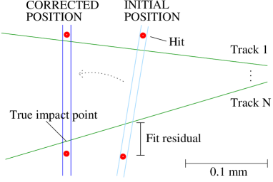
Figure 1: Schematic illustration of the method to correct the sensor position: using a large number of tracks $i,i=1,\dots,N$ and measured hits on a detector, the sensor is moved such as to minimize the residuals.

The outline of this paper is as follows: In Section II we briefly review published alignment methods. In Section III we introduce the basic notations and coordinate systems involved in our method. In Section IV we present the detailed formulation of the method. In Sections V and VI we demonstrate the performance of the method applied to a test beam setup and to a simulated pixel vertex detector, respectively. The CMS CMS-tracker Pixel detector is is used as a model in the simulation.

II BRIEF REVIEW OF ALIGNMENT METHODS

Most HEP experiments equipped with precise tracking detectors have to deal with misalignment issues, and several different approaches for alignment by tracks have been used and reported. Most methods are iterative with 5-6 parameters solved at a time.

Several papers concerning different aspects of alignment in the DELPHI experiment can be found in the literature. For instance, $Z^{0}\rightarrow\mu^{+}\mu^{-}$ and cosmic rays are used for the global alignment between sub-detectors VD, OD and TPC litDelphiGlob . The most detailed DELPHI alignment paper deals with the alignment of the Microvertex detector litDelphiPed .

In the ALEPH experiment, alignment was carried out wafer by wafer, and with 20 iterations and 20000 $Z^{0}\rightarrow q\bar{q}$ and 4000 $Z^{0}\rightarrow\mu^{+}\mu^{-}$ events an accuracy of a few $\mu m$ can be achieved litAleph .

A different, computationally challenging approach is chosen in the SLD experiment, where the algorithm requires simultaneous solution of 576 parameters leading to a 576 by 576 matrix inversion litSLD576 . In the SLD vertex detector, a recently developed matrix singular value decomposition technique is also used for internal alignment litSLDsvd .

III COORDINATE SYSTEMS AND TRANSFORMATIONS

Our method is applicable to detector setups which consist of planar sensors like silicon pixel or strip detectors. For track reconstruction one conventionally uses the local (sensor) coordinate system and the global detector system. The local system $(u,v,w)$ is defined with respect to a detector module (sensor) as follows: The origin is at the center of the sensor, the $w$-axis is normal to the sensor, the $u$-axis is along the precise coordinate and the $v$-axis along the coarse coordinate. The global coordinates are denoted as $(x,y,z)$.

The transformation from the global to the local system goes as:

$${\bf q}={\bf R}({\bf r}-{\bf r}_{0})$$ (1)

where ${\bf r}=(x,y,z)$, ${\bf q}=(u,v,w)$, ${\bf R}$ is a rotation and ${\bf r}_{0}=(x_{0},y_{0},z_{0})$ is the position of the detector center in global coordinates.

In the very beginning of the experiment the rotation ${\bf R}$ and the position ${\bf r}_{0}$ are determined by detector assembly and survey information. In the course of experiment this information will be corrected by an incremental rotation ${\Delta{\bf R}}$ and translation ${\Delta{\bf r}}$ so that the new rotation and translation become:

$${\bf R} \rightarrow {\Delta{\bf R}}{\bf R}$$ (2)

$${\bf r}_{0} \rightarrow {\bf r}_{0}+{\Delta{\bf r}}.$$ (3)

The correction matrix ${\Delta{\bf R}}$ is expressed as:

$${\Delta{\bf R}}={\bf R}_{\gamma}{\bf R}_{\beta}{\bf R}_{\alpha}$$ (4)

where ${\bf R}_{\alpha},{\bf R}_{\beta}$ and ${\bf R}_{\gamma}$ are small rotations by ${\Delta\alpha},{\Delta\beta},{\Delta\gamma}$ around the $u$-axis, the (new) $v$-axis and the (new) $w$-axis, respectively. The position correction ${\Delta{\bf r}}$ transforms to the local system as:

$${\Delta{\bf q}}={\Delta{\bf R}}{\bf R}{\Delta{\bf r}}$$ (5)

with ${\Delta{\bf q}}=(\Delta u,\Delta v,\Delta w)$. Using (1-5) we find the corrected transformation from global to local system as:

$${\bf q}^{c}={\Delta{\bf R}}{\bf R}({\bf r}-{\bf r}_{0})-{\Delta{\bf q}}.$$ (6)

where the superscript $c$ stands for ’corrected’. The task of the alignment procedure by tracks is to determine the corrective rotation ${\Delta{\bf R}}$ and translation ${\Delta{\bf r}}$ or ${\Delta{\bf q}}$ as precisely as possible for each individual detector element.

IV DESCRIPTION OF THE ALIGNMENT ALGORITHM

IV.1 Basic Formulation

Since the alignment corrections are small, the fitted trajectories can be approximated with a straight line in a vicinity of the detector plane. The size of this small region is determined by the alignment uncertainty which is expected to be at most a few hundred microns so that the straight line approximation is perfectly valid.

The equation of a straight line in global coordinates, approximating the trajectory in a vicinity of the detector, can be written as:

$${\bf r}_{s}(h)={\bf r}_{x}+h\ {\hat{\bf s}}$$ (7)

where ${\bf r}_{x}$ is the trajectory impact point on the detector in question, $\hat{\bf s}$ is a unit vector parallel to the line and $h$ is a parameter. Equation (7) is for uncorrected detector positions.

Using Eq. (6) the corrected straight line equation in the local system reads:

$${\bf q}_{s}(h)={\bf R}_{c}({\bf r}_{x}+h\ {\hat{\bf s}}-{\bf r}_{0})-{\Delta{\bf q}}$$ (8)

where ${\bf R}_{c}={\Delta{\bf R}}{\bf R}$. A point ${\bf q}_{s}={\bf q}_{s}(h_{x})$ which lies in the detector plane must fulfill the condition ${\bf q}_{s}\cdot{\hat{\bf w}}=0$, where ${\hat{\bf w}}=(0,0,1)$ is normal to the detector. From this condition we can solve the parameter $h_{x}$ which gives the corrected impact or x-ing point on the detector:

$$h_{x}=\frac{[{\Delta{\bf q}}-{\bf R}_{c}({\bf r}_{x}-{\bf r}_{0})]\cdot{\hat{\bf w}}}{{\bf R}_{c}{\hat{\bf s}}\cdot{\hat{\bf w}}}.$$ (9)

The corrected impact point coordinates ${\bf q}_{x}^{c}$ in the local system are then:

$${\bf q}_{x}^{c}={\bf R}_{c}({\bf r}_{x}-{\bf r}_{0})+\frac{[{\Delta{\bf q}}-{\bf R}_{c}({\bf r}_{x}-{\bf r}_{0})]\cdot{\hat{\bf w}}}{{\bf R}_{c}{\hat{\bf s}}\cdot{\hat{\bf w}}}{\bf R}_{c}{\hat{\bf s}}-{\Delta{\bf q}}.$$ (10)

Since the uncorrected impact point is ${\bf q}_{x}={\bf R}({\bf r}_{x}-{\bf r}_{0})$, Eq. (10) can be written as:

$${\bf q}_{x}^{c}={\Delta{\bf R}}\,{\bf q}_{x}+\frac{({\Delta{\bf q}}-{\Delta{\bf R}}\,{\bf q}_{x})\cdot{\hat{\bf w}}}{{\Delta{\bf R}}{\hat{\bf t}}\cdot{\hat{\bf w}}}{\Delta{\bf R}}\,{\hat{\bf t}}-{\Delta{\bf q}}.$$ (11)

where ${\hat{\bf t}}={\bf R}{\hat{\bf s}}$ is the uncorrected trajectory direction in the detectors local frame of reference. Eq. (11) evaluates to:

$${\bf q}_{x}^{c}={\Delta{\bf R}}\,{\bf q}_{x}+(\Delta w-[{\Delta{\bf R}}\,{\bf q}_{x}]_{3})\frac{{\Delta{\bf R}}\,{\hat{\bf t}}}{[{\Delta{\bf R}}\,{\hat{\bf t}}]_{3}}-{\Delta{\bf q}}.$$ (12)

This expression provides us with a ’handle’ by which the unknowns ${\Delta{\bf q}}$ and ${\Delta{\bf R}}$ can be estimated by minimizing a respective $\chi^{2}$ function using a large number of tracks.

IV.2 General $\chi^{2}$ Solution

We denote a measured point in local coordinates as ${\bf q}_{m}=(u_{m},v_{m},0)$. The corresponding trajectory impact point is ${\bf q}_{x}^{c}=(u_{x},v_{x},0)$. For simplicity we omit the superscripts $c$ in the coordinates $u_{x}$ and $v_{x}$. In stereo and pixel detectors we have two measurements, $u_{m}$ and $v_{m}$, and in non-stereo strip detectors only one, $u_{m}$. In the latter case the coarse coordinate $v_{m}$ is redundant. The residual is either a 2-vector:

$${\bf\varepsilon}=\left(\begin{array}[]{c}\varepsilon_{u}\\ \varepsilon_{v}\end{array}\right)=\left(\begin{array}[]{c}u_{x}-u_{m}\\ v_{x}-v_{m}\end{array}\right)$$ (13)

or a scalar $\varepsilon=\varepsilon_{u}=u_{x}-u_{m}$. In the following we treat the more general 2-vector case. The scalar case is a straightforward specification of the 2-vector formalism.

The $\chi^{2}$ function to be minimized for a given detector is:

$$\chi^{2}=\sum_{j}{\bf\varepsilon}_{j}^{T}{\bf V}_{j}^{-1}{\bf\varepsilon}_{j}$$ (14)

where the sum is taken over the tracks $j$. ${\bf V}_{j}$ is the covariance matrix of the measurements $(u_{m},v_{m})$ associated with the track $j$. The alignment correction coefficients, i.e. the three position parameters $(\Delta u,\Delta v,\Delta w)$ and the three orientation parameters $({\Delta\alpha},{\Delta\beta},{\Delta\gamma})$ are found iteratively by a general $\chi^{2}$ minimization procedure. At each step of the iteration one uses the so far best estimate of the alignment parameters in the track fit.

Let us denote these parameters as ${\bf p}=(\Delta u,\Delta v,\Delta w,{\Delta\alpha},{\Delta\beta},{\Delta\gamma})$. Then, according to the general $\chi^{2}$ solution, the iterative correction to ${\bf p}$ has the following expression:

$$\delta{\bf p}=\left[\sum_{j}{\bf J}_{j}^{T}{\bf V}_{j}^{-1}{\bf J}_{j}\right]^{-1}\left[\sum_{j}{\bf J}_{j}^{T}{\bf V}_{j}^{-1}{\bf\varepsilon}_{j}\right]$$ (15)

where ${\bf J}_{j}$ is a Jacobian matrix of ${\bf\varepsilon}_{j}({\bf p})$:

$${\bf J}_{j}=\nabla_{\bf p}\ {\bf\varepsilon}_{j}({\bf p}).$$ (16)

An adequate starting point for the iteration is a null correction vector ${\bf p}$=0.

In the general case of two measurements $(u_{m},v_{m})$, ${\bf J}_{j}$ is a $6\times 2$ matrix. In case of scalar $\varepsilon$, for single sided strip detectors, ${\bf J}_{j}$ is a vector of 5 elements, because $\Delta v$ is redundant and cannot be fitted. It will also be foreseen that only a sub-set of the 6 alignment parameters would be fitted and the others kept fixed. In this case the dimension of the Jacobian matrix reduces accordingly.

The derivatives of the Jacobian matrix can be computed to a good precision in the small correction angle approximation (see below). The elements of the matrix ${\bf J}$ for a given track are then:

$${\bf J}=\left(\begin{array}[]{cc}-1&0\\ 0&-1\\ {\tan{{\psi}}}&{\tan{{\vartheta}}}\\ v_{x}{\tan{{\psi}}}&v_{x}{\tan{{\vartheta}}}\\ u_{x}{\tan{{\psi}}}&u_{x}{\tan{{\vartheta}}}\\ v_{x}&-u_{x}\end{array}\right)$$ (17)

The quantities ${\tan{{\psi}}}$ and ${\tan{{\vartheta}}}$ are defined in the next section.

IV.3 Linearized Solution with the Tilt Formalism

We call ”tilts” the angle corrections $x$ which are small enough to justify the approximations $\cos{x}\simeq 1$ and $\sin{x}\simeq x$. In this approximation the correction matrix ${\Delta{\bf R}}$ reads:

$${\Delta{\bf R}}=\left(\begin{array}[]{ccc}1&{\Delta\gamma}&{\Delta\beta}\\ -{\Delta\gamma}&1&{\Delta\alpha}\\ -{\Delta\beta}&-{\Delta\alpha}&1\end{array}\right)$$ (18)

Using Eq. (18) we linearize Eq. (12) and get the following expressions for the corrections of the impact point coordinates as a function of the alignment correction parameters:

$$\Delta u_{x} = -\Delta u+\delta\,{\tan{{\psi}}}+{\Delta\gamma}\,v_{x}$$ (19)

$$\Delta v_{x} = -\Delta v+\delta\,{\tan{{\vartheta}}}-{\Delta\gamma}\,u_{x}$$ (20)

where $\delta=\Delta w+{\Delta\beta}\,u_{x}+{\Delta\alpha}\,v_{x}$. The quantity ${\psi}$ is the angle between the track and the $vw-$plane and ${\vartheta}$ is the angle between the track and the $uw-$plane: ${\tan{{\psi}}}=\hat{t}_{1}/\hat{t}_{3}$, ${\tan{{\vartheta}}}=\hat{t}_{2}/\hat{t}_{3}$.

With this approximation the residuals (13) depend linearly on all 6 parameters. Hence the $\chi^{2}$ minimization problem is linear and can be solved by standard techniques without iteration.

V ALIGNMENT OF A TEST BEAM SETUP

From Eqs. (19) and (20) we can estimate the contributions of various misalignments to the hit measurement errors. For example the contribution of a misalignment ${\Delta\alpha}$ around the $u$-axis to the $v$-coordinate is:

$$\Delta v\simeq v\,{\Delta\alpha}\,{\tan{{\vartheta}}}.$$ (21)

The error is small near normal incident angles, but grows rapidly as a function of ${\vartheta}$. At ${\vartheta}=45^{o}$ and near the edge of the sensor ($v=3$ cm) the error goes as $30000\,{\mu\mbox{m}}\,{\Delta\alpha}$ so that for only $1\,\mbox{mrad}$ error in ${\Delta\alpha}$ the systematic error in the $v$-coordinate is $30\,{\mu\mbox{m}}$.

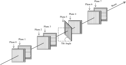
Figure 2: Helsinki Si Beam Telescope in the CERN H2 beam.

The silicon detector team of Helsinki Institute of Physics made a precision survey of detector resolution as a function of the angle of incidence of the tracks calib_paper . The study was made in the CERN H2 particle beam with a setup described in Figure 2. One of the silicon strip detectors was fixed on a rotative support which allowed the tracks to enter between $0$ and $30$ degrees of incident angle. The angular dispersion of the beam was about 10 mrad and the hits covered the full area of the test detector.

In order to obtain reliable results it was extremely important to calibrate the tilt angle to a very high precision. Our algorithm was used in the alignment calibration. In Table 1 we show the result of the alignment demonstrating the precision obtained by about 3000 beam tracks.

Table 1: Alignment parameters obtained by the algorithm

Parameter	At 0 degrees	At 30 degrees
$\Delta u({\mu\mbox{m}})$	186.0$\pm$0.1	-264.7$\pm$0.1
$\Delta w({\mu\mbox{m}})$	200$\pm$20	-131$\pm$6
$\Delta\alpha(\mbox{mrad})$	5.6$\pm$0.7	12.9$\pm$0.9
$\Delta\beta(\mbox{mrad})$	5.8$\pm$0.9	32.59$\pm$0.04
$\Delta\gamma(\mbox{mrad})$	-14.12$\pm$0.01	-15.86$\pm$0.01

With the precise alignment we have been able to determine the optimal track incident angle which minimizes the detector resolution calib_paper .

VI MONTE CARLO SIMULATION

VI.1 Simulated Detector

A Monte Carlo simulation code was written to test the alignment algorithm. High momentum tracks were simulated and driven through a set of detector planes. The simulated hits were fluctuated randomly to simulate measurement errors. Gaussian multiple scattering was added quadratically using the Highland Highland approximation. The algorithm involves misalignment of a detector setup in order to simulate a realistic detector.

The experimenters’ imperfect knowledge of the true position of the detector planes is simulated by reconstructing the trajectories in the ideal (not misaligned) detector. This means that in the transformation from local to global coordinate system one uses the ideal positions of the detector planes. The full algorithm in brief is as follows:

1. Creation of an ideal detector setup with no misalignments

2. Creation of a misaligned, realistic detector

3. Generation of the particles and hits in the misaligned detector simulating the real detector

4. Reconstruction of the particle trajectories in the nominal (ideal) detector thus using slightly wrong hit positions. This simulates the realistic situation in which the detector alignment is not yet performed.

For the simulated detector type we choose a vertex detector which is a simplification of the CMS Pixel barrel detector CMS-tracker ; pixel-det with two layers. The setup is illustrated in Figure 3. There are 144 sensors in layer 1 and 240 sensors in layer 2. The distance of the layer 1 from the beam line is about 4 cm and the layer 2 about 8 cm.

Figure 3: Illustration of the simulated vertex detector in the alignment study.

In the simulation we used the following conditions:

1. Misalignment of chosen sensors: The shifts $\Delta{u},\Delta{v},\Delta{w}$ were chosen at random, each in the range $\pm 100\,{\mu\mbox{m}}$ and the tilts ${\Delta\alpha},{\Delta\beta},{\Delta\gamma}$ were chosen at random each in the range $\pm{20}\,\mbox{mrad}$.

2. Beam and vertex constraints: The vertex positions were Gaussian fluctuated around the center of the beam diamond with $\sigma_{x}=\sigma_{y}=20\,{\mu\mbox{m}}$ and $\sigma_{z}=7\,$cm and the tracks were fitted with the constraint to start from one point, i.e. from the primary vertex.

In the following we consider two different cases of misaligned detectors:

1. All sensors in layer 2 fixed, all sensors in layer 1 misaligned.

2. Only one sensor in layer 2 fixed, all remaining 383 sensors misaligned.

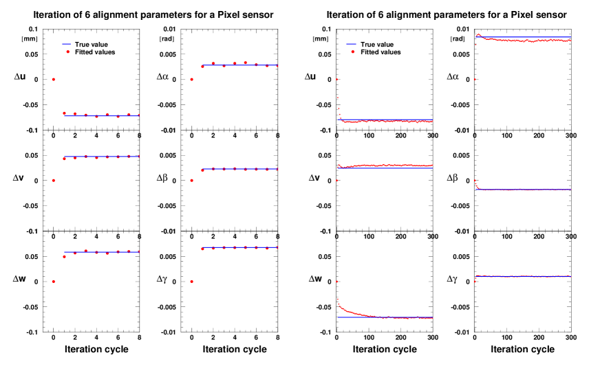
Figure 4: The six plots on the left show the rate of convergence in case I for the alignment parameters of one sensor (circular spots). The solid line shows the true parameter value. The six plots on the right are for the case II.

In case I the total number of fitted parameters is $6\times 144=864$ and we used about $2\times 10^{5}$ tracks. The case I appears to be an ’easy’ one with which the algorithm copes very well, as we see below. The second case we call ’extreme’ since the alignment is based on one reference sensor which covers only about 0.26 % of the detector setup area. The total number of fitted parameters in this case was $6\times 383=2298$. In the following sectios we show perfomance results of the algorithm in these two cases.

VI.2 Convergence of the Algorithm

The convergence rate of the alignment procedure as a function of the iteration cycle is shown in Figure 4. It appears that the convergence is fast in the ’easy’ case (the 6 plots on the left) where more than 60 % of the sensors provide the reference. The convergence takes place after a couple of iterations.

In the case where only one sensor is taken as a reference (plots on the right of the figure), the situation is different. It appears that the number of iterations needed varies between 20 and 100 from parameter to parameter. It is also seen that the converged parameter values are somewhat off from the true values, but the precision is reasonable.

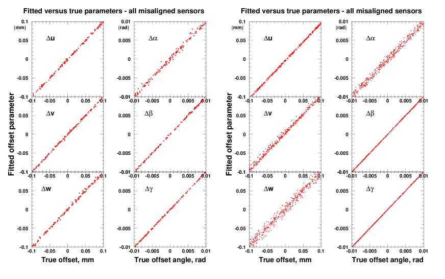
Figure 5: The scatter plot of fitted versus true alignment parameters. There are $6\times 144$ entries in the plots on the left (case I) and $6\times 383$ entries in the plots on the right (case II).

VI.3 Comparison of Fitted and True Parameters

The precision of the fitted parameters in comparison with the true values is shown in Figure 5 on the left for the case I. The correlations are very strong. The typical deviation of the fitted parameters from the true value is less than $1\,{\mu\mbox{m}}$ for the offsets and a fraction of a milliradian for the tilts. The precision appears to be better than actually needed in this case, indicating that a smaller statistics would give a satisfactory result.

In case II (the plots on the right of the figure) a good correlation is observed, but the precision is somewhat more modest. For example the error in $\Delta w$ (the shift normal to the sensor plane) is still in most cases below $10\,{\mu\mbox{m}}$.

VII CONCLUSIONS

We have developed a sensor alignment algorithm which is mathematically and computationally simple. It is based on repeated track fitting and residuals optimization by $\chi^{2}$ minimization. The computation is simple, because the solution involves matrices whose dimension is at most $6\times 6$. The method is capable of solving simultaneously all six alignment parameters per sensor for a detector setup with a large number of sensors.

We have successfully applied the method in a precision survey of silicon strip detector resolution as a function of the tracks incident angle. Furthermore, we have demonstrated the performance of the algorithm in case of a simulated two-layer pixel barrel vertex detector. The method performs very well in the case where the outer layer is taken as a reference and all inner sensors are to be aligned. The algorithm performs reasonably well also in the extreme case where only one sensor, representing some 0.26 % of the total area, is taken as a reference for the alignment.

- (1) M. Della Negra et al., ”CMS Tracker Technical Design Report”, CERN/LHCC 98-6.
- (2) B. Mours et al., ”The design, construction and performance of the ALEPH silicon vertex detector”, Nucl. Instr. and Meth. A453 (1996) 101-115.
- (3) A. Andreazza and E. Piotto, ”The Alignment of the DELPHI Tracking Detectors”, DELPHI 99-153 TRACK 94 (1999).
- (4) M. Caccia and A. Stocchi, ”The DELPHI vertex detector alignment: A pedagogical statistical exercise”, INFN AE 90-16 (1990).
- (5) K. Abe et al., ”Design and performance of the SLD vertex detector, a 307 Mpixel tracking system”, Nucl. Instr. and Meth. A400 (1997).
- (6) D. J. Jackson and Dong Su and F. J. Wickens, ”Internal alignment of the SLD vertex detector using a matrix singular value decomposition technique”, Nucl. Instr. and Meth. A491 (2002).
- (7) C. Eklund et al., ”Silicon Beam Telescope for CMS Detector Tests”, Nucl. Instr. and Meth. A430 (1999) 321-332.
- (8) K. Banzuzi et al., ”Performance and Calibration Studies of Silicon Strip Detectors in a Test Beam”, Nucl. Instr. and Meth. A453 (2000) 536.
- (9) V.L. Highland, ”Some Practical Remarks on Multiple Scattering”, Nucl. Instr. and Meth. 129 (1975) 497.
- (10) D. Kotlinski, ”The CMS Pixel Detector”, Nucl. Instr.and Meth. A465 (2000) 46.