Classical-Wigner Phase Space Approximation to Cumulative Matrix Elements in Coherent Control

Abstract

The classical limit of the Wigner-Weyl representation is used to approximate products of bound-continuum matrix elements that are fundamental to many coherent control computations. The range of utility of the method is quantified through an examination of model problems, single-channel Na₂ dissociation and multi-arrangement channel photodissociation of CH₂IBr. Very good agreement with the exact quantum results is found for a wide range of system parameters.

I Introduction

Recent experimental and theoretical developments show that coherent control, i.e. the control of atomic and molecular dynamics via quantum interference, can be successfully applied to the wide variety of systems cc . However, available quantum methods limit theoretical studies to scattering and photodissociation of small molecules. The extension of theoretical studies to larger complex chemical systems must rely on new developments in quantum or semiclassical techniques. Primary amongst these is the application of the Initial Value Representation semiclassical approach that is described elsewhere batista ; Miller1 . However, the ultimate utility of such techniques requires the development of numerical tools to speed convergence of the initial value integrals with highly oscillatory integrands.

In this paper we consider an approach to computing interference contributions in coherent control in which such oscillations do not occur. Specifically, we focus attention on using the classical limit of Wigner Phase Space MethodsWigner ; Imre , where the desired transition matrix elements products are written in the Wigner-Weyl representation and the quantum expressions are replaced by their classical counterparts. This approach has been applied in the past to a number of simpler problemsHeller1 ; Heller3 where transitions from one initial bound state were considered, e.g., from a single vibrational state Heller1 or from a Gaussian state Hupper ; Hupper1 . In these cases only absolute values squared of matrix elements were sought. By contrast, in this paper we use a result Wilkie on the classical limit of the nonstationary Liouville eigenstates to obtain the classical limit of the desired product of transition dipole matrix elements, a quantity which, in general, includes phase information. For example, we demonstrate that the method gives good results for complex valued matrix elements that arise in the multi-arrangement photodissociation of CH₂IBr to CH₂I + Br or CH₂Br + I. The method has also been previously applied in the guise of the linearized approximation to the Initial Value RepresentationMiller2 with varying degrees of success.

This paper is organized as follows. The classical limit of the Wigner phase space method is described in Section II. Applications of the method to simple systems involving one arrangement channel are described in Section III. Specifically, we consider Franck-Condon transitions for the model case of excitations from a harmonic oscillator potential to a linear potential and to transitions on realistic Na₂ potential energy surfaces. Section IV discusses applications to collinear photodissociation of CH₂IBr, where the transitions probabilities are complex because the relevant operators are no longer Hermitian. Section V provides a summary of results.

II Method

In various coherent control scenarios (e.g., bichromatic control ccold or coherent control via pulse sequencing Seideman ) control is dictated (here written for the case of non-rotating diatomics) by interference terms of the form

$$\sigma_{n,m}^{(r)}(E)=\sum_{\textbf{k}}\langle\,{E,\textbf{k},r^{-}}\,|\mu_{fi}|n\rangle\langle m|\mu_{fi}|\,{E,\textbf{k},r^{-}}\,\rangle=\sum_{\textbf{k}}\langle\,{E,\textbf{k},r^{-}}\,|\chi_{n}\rangle\langle\chi_{m}|\,{E,\textbf{k},r^{-}}\,\rangle~{}.$$ (1)

Here $|\chi_{j}\rangle=\mu_{fi}|j\rangle,\,j=n,m$ and $\mu_{fi}$ is the electronic transition dipole moment between the upper and lower electronic states. The states $|j\rangle$ of energy $E{{}_{j}}$, are bound vibrational states on the lower potential energy surface, and $|\,{E,\textbf{k},r^{-}}\,\rangle$ are continuum nuclear eigenstates of energy $E$ on an excited electronic surface, corresponding to product in channel $r$ with quantum numbers k. Terms like those in Eq. (1) arise when one calculates the probability $P(E)$ of transition from a coherently prepared bound superposition state

$$|\psi\rangle=\sum_{i}c_{i}|i\rangle,$$ (2)

to the final continuum states at energy $E$ in arrangement $r$ ccold . That is, these terms correspond to the interference terms in computing the probability $P(E)\propto\sum_{k}|\langle E,\textbf{k},r^{-}|\mu_{fi}|\psi\rangle|^{2}$. Since coherent control relies upon quantum interference to obtain control over molecular outcomes, the evaluation of terms like those in Eq. (1) are vital to computational control studies.

In the simplest case, when $n=m$ and only one product arrangement channel is open, Eq. (1) is proportional to the photodissociation probability for the transition from an initial bound state $|n\rangle$ at energy $E_{n}$ to the continuum of final states at energy $E$:

$$\sigma_{n,n}^{(r)}(E)=\sum_{\textbf{k}}|\langle\,{E,\textbf{k},r^{-}}\,|\mu_{fi}|n\rangle|^{2}.$$ (3)

To utilize Eq. (1) we rewrite it as:

$$\sigma_{n,m}^{(r)}(E)={\rm Tr}[(\sum_{\textbf{k}}|\,{E,\textbf{k},r^{-}}\,\rangle\langle\,{E,\textbf{k},r^{-}}\,|(|\chi_{m}\rangle\langle\chi_{n}|)],$$ (4)

where “Tr” denotes the trace. The term $\sum_{\textbf{k}}|\,{E,\textbf{k},r^{-}}\,\rangle\langle\,{E,\textbf{K},r^{-}}\,|$ can then be written as

$$\sum_{\textbf{k}}|\,{E,\textbf{k},r^{-}}\,\rangle\langle\,{E,\textbf{k},r^{-}}\,|=\hat{R}_{r}\delta({E-\hat{H}})$$ (5)

where $\hat{R}_{r}$ projects onto product arrangement $r$ and $\hat{H}$ is the Hamiltonian of the excited electronic state WBO82 . When summed over $r$ (or when there is only one product arrangement channel) this equation reduces to the familiar expression:

$$\sum_{\textbf{k},r}|\,{E,\textbf{k},r^{-}}\,\rangle\langle\,{E,\textbf{k},r^{-}}\,|=\delta(E-\hat{H}).$$ (6)

Using Eq. (5), Eq. (4) can then be rewritten as

$$\sigma_{n,m}^{(r)}(E)={\rm Tr}[\hat{R}_{r}\delta(E-\hat{H})](|\chi_{m}\rangle\langle\chi_{n}|)].$$ (7)

The Wigner transform O_W of any operator $\hat{\textrm{O}}$ is defined as Wigner

$$O_{\rm W}({\bf p},{\bf q})={1\over\pi\hbar}\int_{-\infty}^{+\infty}d{\bf v}\,\,\,e^{2i{\bf p}\cdot{\bf v}/\hbar}\langle{\bf q}-{\bf v}|\hat{O}|{\bf q}+{\bf v}\rangle,$$ (8)

where ${\bf p}$ is the momentum conjugate to coordinate ${\bf q}$. Taking the Wigner transform of Eq. (7) and using ${\rm Tr}(AB)={\rm Tr}(A_{\rm W}B_{\rm W})$ gives

$$\sigma_{n,m}^{(r)}(E)={\rm Tr}\left[[\hat{R}_{r}\delta(E-\hat{H})]_{\rm W}\rho^{\chi}_{n,m}\right]~{},$$ (9)

where $\rho^{\chi}_{n,m}({\bf p},{\bf q})\equiv[|\chi_{n}\rangle\langle\chi_{m}|]_{\rm W}$ is the Wigner transform of $|\chi_{n}\rangle\langle\chi_{m}|$. Neglecting the coordinate dependence of $\mu_{fi}$ in accord with the Franck-Condon approximation gives

$$\sigma_{n,m}^{(r)}(E)=\mu_{fi}^{2}{\rm Tr}\left[[\hat{R}_{r}\delta(E-\hat{H})]_{\rm W}\rho_{n,m}\right]~{},$$ (10)

where $\rho_{n,m}=\rho_{n,m}(\textbf{p},\textbf{q})=[|\,{n}\,\rangle\langle\,{m}\,|]_{W}$. Equation (10) is exact. In Section III of this paper we consider applications of approximations to Eq. (10) to cases with a single product arrangement channel. Section IV considers the case of multiple chemical products.

III Single Product Arrangement Channel

In the case where there is only a single product arrangement channel, Eq. (10) becomes

$$\sigma_{n,m}(E)=\mu_{fi}^{2}{\rm Tr}[\delta(E-\hat{H})_{\rm W}\rho_{n,m}]=\mu_{fi}^{2}\int d{\bf p}\,d{\bf q}\,\,\delta(E-\hat{H})_{\rm W}\,\rho_{n,m}({\bf p},{\bf q})~{}.$$ (11)

Here

$$\rho_{n,m}({\bf p},{\bf q})=[|n\rangle\langle m|]_{\rm W}={1\over\pi\hbar}\int d{\bf v}\,\,\exp(2i{\bf p}\cdot{\bf v}/\hbar)\langle{\bf q}-{\bf v}|n\rangle\langle m|{\bf q}+{\bf v}\rangle~{},$$ (12)

so that $\sigma_{n,m}(E)$ appears as the overlap of two phase space densities, one corresponding to the density on the lower surface [$\rho_{n,m}({\bf p},{\bf q})$] and one to the continuum density $\delta(E-\hat{H})_{\rm W}$ on the upper excited surface. Neither of these densities need be classical since they can be negative or complex.

The classical Wigner approximation to $\sigma_{n,m}(E)$ is obtained by taking the classical limit ($\hbar\rightarrow 0$) of Eq. (11), where the classical limit of $\delta(E-\hat{H})_{\rm W}$ arises by either expanding the density of states in powers of $\hbar$, or by using the statistical operator Wigner ; Heller1 $\hat{P}=\exp(-\beta\hat{H})$, $\beta=1/kT$, or via an exponentiated $\hbar$ expansion Mayer , or by expanding $\delta(E-\hat{H})_{\rm W}$ around the identity operator $\hat{I}$ times the classical Hamiltonian, $H({\bf p},{\bf q})\cdot\hat{I}$ Hupper . The lowest order term in this expansion is $\delta(E-H({\bf p},{\bf q}))$, where $H({\bf p},{\bf q})$ is the classical Hamiltonian associated with the upper potential energy surface $V({\bf q})$. For a particle of reduced mass $\mu$ in one dimension, which we focus on in this section:

$$H(p,q)=\frac{p^{2}}{2\mu}+V(q)~{},$$ (13)

so that the lowest order classical Wigner phase space method approximation to $\sigma_{n,m}(E)$ [denoted $\sigma_{n,m}^{c}(E)$] is

$$\sigma_{n,m}^{\rm c}(E)=\mu_{fi}^{2}\int\,dp\,dq\,\,\delta(E-H(p,q))\rho_{n,m}^{c}(p,q)$$ (14)

$$=\mu_{fi}^{2}\int\,dp\,dq\,\,{\delta(q-q(p,E))\over\left|\left({\partial V\over\partial q}\right)_{q=q(p,E)}\right|}\rho_{n,m}^{c}(p,q)=\mu_{fi}^{2}\int\,dp\,{\rho_{n,m}^{c}(q(p,E),p)\over\left|\left({\partial V\over\partial q}\right)_{q=q(p,E)}\right|},$$ (15)

where $E-p^{2}/2\mu-V(q(p,E))=0$, and where $\rho_{n,m}^{c}(p,q)$ is the classical limit of $\rho_{n,m}$ .

The form of $\rho_{n,m}^{c}$ depends on whether the system is integrable or non-integrable Wilkie . For integrable systems [Eq. (17), Eq. (18), Ref. Wilkie ]

$$\rho_{n,m}^{c}={1\over 2\pi}\delta(I(p,q)-\bar{I}_{n,m})\exp[i(n-m)\theta(p,q)],$$ (16)

where [$I(p,q),\theta(p,q)$] are action-angle variables, $\bar{I}_{n,m}=(I_{n}+I_{m})/2$, and $I_{n}$ is the semiclassical action associated with state $|n\rangle$ (i.e., $I_{n}=(n+\gamma)\hbar$, where $\gamma$ is the Maslov index). A similar analytic expression is not possible for chaotic systems Wilkie .

In the cases studied below we focus on transitions from low lying vibrational states of diatomics. In this case we can approximate the potential by an harmonic oscillator of frequency $\omega$ and approximate $\rho_{n,m}^{c}(p,q)$ by the harmonic case. However, in the harmonic case the classical $\rho_{n,m}^{c}(p,q)$ can be chosen as equal to $\rho_{n,m}(p,q)$ for the quantum harmonic oscillator JaffeBrumer1 . Substituting expressions for the harmonic oscillator states

$$\langle q|n\rangle=\left({\mu\omega\over\hbar}\right)^{1/4}\left(2^{n}n!\sqrt{\pi}\right)^{-1/2}H_{n}\left(\sqrt{\mu\omega\over\hbar}q\right)e^{-{\mu\omega q^{2}\over 2\hbar}}$$ (17)

into the Wigner transform of Eq. (12), we obtain

$$\rho_{n,m}^{c}(p,q)=\rho_{n,m}(p,q)={(-1)^{n}\over\pi\hbar}\left[{2^{n}m!\over n!2^{m}}\right]^{1/2}\left({1\over\hbar\mu\omega}\right)^{{n-m\over 2}}$$

$$\times\quad\left[ip-\mu\omega q\right]^{n-m}\exp\left({-{2I(p,q)\over\hbar}}\right)L_{m}^{n-m}\left[{4I(p,q)\over\hbar}\right],$$ (18)

where $n\geq m$, $L_{k}^{\alpha}$ is the generalized Laguerre polynomial, and the classical action $I(p,q)$ for the harmonic oscillator is

$$I(p,q)={H(p,q)\over\omega}={1\over 2}\left({p^{2}\over\mu\omega}+\mu\omega q^{2}\right).$$ (19)

For the case of $n=m$, Eq. (18) takes the well-known form

$$\rho_{n,m}(p,q)={(-1)^{n}\over\pi\hbar}\exp\left({-{2H(p,q)\over\hbar\omega}}\right)L_{n}\left({4H(p,q)\over\hbar\omega}\right).$$ (20)

IV Results: Single Arrangement Channel

IV.1 Model Potentials

We first test the utility of this approximation on a simple standard model: excitation from an harmonic oscillator initial state potential to a linear, repulsive excited state potential $V(q)=-\beta q+E_{0}$, with $E_{0}$ arbitrary and $\beta>0$. This model was previously examined for $n=m=0$ in Ref. Heller1 , and can be used to approximate transitions to an arbitrary potential if $\beta$ is taken as the slope of the upper potential energy surface at the peak of the initial state ($n=m=0$) wavefunction. For simplicity, we set the $\mu_{fi}$ to unity. $\delta(E-\hat{H})_{W}$ is known Heller1 for the linear excited state potential, so that the exact $\sigma_{n,m}(E)$ is given by

$$\sigma_{n,m}(E)=2\pi\int\,dp\,dq\,\delta(E-\hat{H})_{W}\rho_{n,m}(p,q)$$

$$=2\pi\int\,dp\,dq\,\left({\beta^{1/3}\over\pi\beta}\right)Ai\left[-(2\beta^{1/3})(q-q(p,E))\right]\,\rho_{n,m}(p,q).$$ (21)

where $Ai$ is the Airy function.

By contrast, the classical result [Eq. (15)] for this model is

$$\sigma_{n,m}^{\rm c}(E)=\int\,dp\,dq\,\delta\left(E-{p^{2}\over 2\mu}+\beta q-E_{0}\right)\rho_{n,m}^{c}(p,q)$$

$$={1\over\beta}\int\,dp\,dq\,\delta(q-q(p,E))\,\rho_{n,m}^{c}(p,q)={1\over\beta}\int\,dp\,\rho_{n,m}^{c}(p,q(P,E)),$$ (22)

where $q(p,E)=(E_{0}-E)/\beta+p^{2}/2\mu\beta$.

In Fig. 1 we compare the exact quantum and classical Wigner results for the highly quantum case of $\mu=m_{e}=$1 a.u., where $m_{e}$ is the mass of electron. Note that $\sigma_{n,m}$, $n\neq m$ is real for the one-dimensional case with real $V(q)$ since the integral over the imaginary part is odd in the momentum variable. In Figs. 1(a)-(b), $\sigma_{n,m}$ for $n=m=0$ and $n=m=4$ are shown as functions of energy $E-E_{0}$ for parameters given in Ref. Heller1 ; $\beta=6$ a.u., $\omega=2$ a.u. Our results for $n=0$ agree very well with those in Ref. Heller1 , and with the $n=m=1$ results for $\beta=6$ a.u., $\omega=1$ a.u. (not shown). However, as is evident from Fig. 1, the accuracy of the classical Wigner approximation deteriorates extremely rapidly with increasing $n$; results are very poor even for $n=4$. The same behavior is observed for cases where $n\neq m$, shown in Fig. 1(c)-(d) for ($n=1,\,m=0$) and ($n=5,\,m=4$). This is because for small $n$, $\rho_{n,n}$ is smooth and broad, and the transition integral averages over many of Airy function oscillations. By contrast, for large $n$, $\rho_{n,n}$ is highly oscillatory and the initial state probes fine details of the Airy functions which are absent in the classical approximation. As is evident from Fig. 1(b), the classical Wigner results for $n=m$ are negative at some points. This is impossible physically and indicative of errors in the approximation. In the $n\neq m$ case, where negative values are possible [Fig. 1(c)-(d)], the positions of maxima in the semiclassical approximations are shifted to lower energies, a feature previously explained for the $n=m$ case Heller1 ; Hupper1 .

Figure 1: Comparison between the classical Wigner (solid line) and exact quantum (dashed line) results for $\sigma_{n,m}(E-E_{0})$ $(n=m)$ for the $\mu=$ 1 a.u. and $\omega=2$ a.u.: (a) $n=m=0$; (b) $n=m=4$; (c) $n=1,m=0$; (d) $n=5,m=4$.

Results presented in Fig. 1 were obtained for $\mu=1$ a.u. which is highly non-classical system. The dependence of the classical-quantum agreement on the oscillator frequency $\omega$ and on the reduced mass $\mu$ are explored, for two cases with $m=n$, in Fig. 2. Agreement is seen to improve dramatically as $\omega$ decreases and somewhat as $\mu$ decreases. The latter result is surprising, motivating the analysis described below.

Figure 2: Comparison between the classical Wigner (solid line) and exact quantum (dashed line) results for $\sigma_{n,m}(E-E_{0})$ $(n=m=4)$ for fixed $\mu=$1 a.u.: (a) $\omega=2.0$; (b) $\omega=0.2$; and for fixed $\omega=$2 a.u.: (c) $\mu=1.0$; (d) $\mu=100.0$.

Characteristic $s_{n}$ factor. The validity of the classical Wigner approximation for cases where $n=m$ and for the excited state linear potential has been examined in Ref. Hupper . There, the utility of the Wigner phase space approximation for an initial Gaussian wavefunction was shown to depend upon two parameters, $s$ and $\lambda$:

$$s={\lambda\over\Delta},\qquad\lambda=\left({\hbar^{2}\over 2\mu\beta}\right)^{1/3},$$ (23)

where $\lambda$ sets the scale for the width of the excited state wavefunction’s oscillations near the turning point (other oscillations have shorter wavelength), and $\Delta$ is the width of the initial Gaussian ground state:

$$\langle q|\Psi_{\rm gr}\rangle={1\over\pi^{1/4}\Delta^{1/2}}e^{-(q-q_{0})^{2}/2\Delta^{2}}.$$ (24)

Specifically, Eckhardt and coworkers Hupper1 have shown that the smaller the $s$, the more accurate the classical approximation, consistent with the fact that smaller $s$ means more Airy oscillations over the width $\Delta$. However, the parameter $s$, as defined in Eq. (23), is not as useful in our case since we consider assorted ground state vibrational wave functions, and not just simple Gaussians. Specifically, $s$ was unable to predict the correct dependence of the classical-quantum agreement on $\mu$ or $\omega$. This is because for any oscillator, the width of the vibrational state $\Delta$ depends on both $\mu$ and $\omega$, whereas Eq. (23) only allows for a dependence on $\mu$ via $\lambda$.

To generalize the $s$ expression to higher vibrational states, for cases with $m=n$, we compare the known expression for the $v=0$ vibrational level

$$\psi=\left({\alpha\over\pi}\right)^{1\over 4}e^{-\alpha(q-q_{0})^{2}\over 2},\quad\alpha={\omega\mu\over\hbar},$$ (25)

to Eq. (24), and obtain $\Delta={1\over\sqrt{\alpha}}=\sqrt{\hbar\over\mu\omega}$. The $s$ parameter can therefore be written as

$$s={\lambda\over\Delta}=\left({\hbar\mu\omega^{3}\over 4\beta^{2}}\right)^{1/6}.$$ (26)

Further, to account for the oscillatory character of the $n$th wavefunction on the lower potential surface, $\Delta$ is replaced by $\Delta_{n}$, where $\Delta_{n}$ equals the width at half-maximum of a single oscillation of the ground state wavefunction. This is given by $\Delta_{n}=l/2(n+1)$, where $l=2\sqrt{2(n+1/2)\hbar/\mu\omega}$ is the overall width of the ground state wavefunction, estimated as the distance between the two classical turning points. This gives the new parameter $s_{n}$:

$$s_{n}={\lambda\over\Delta_{n}}=\sqrt{(n+1)^{2}\over 2(n+1/2)}\,\,\,s\;\;;\;{\rm or}\;\;s_{n}=\sqrt{n\over 2}\,\,s{\rm\,\,\,\,for\,\,large\,\,}n.$$ (27)

It follows from Eq. (27) that the smaller the $s$ is for $n=m=0$, the better the classical approximation for higher-lying levels. However, $s_{n}$ will always increase with increasing $n$ due to the decreasing wavelength of the bound wavefunction. Further, decreasing the vibrational frequency of the lower electronic state $\omega$ leads to wider vibrational states (and larger $\Delta$ in Eq. (23) for the Gaussian ground state) and, therefore, to the smaller $s$ and better agreement with quantum result. This explains the results shown in Fig. 2(a)-(b), where the corresponding values of $s$ for two $\omega$ values are 0.62 ($s_{4}=1.03$) and 0.20 ($s_{4}=0.3$), respectively. Alternatively, note that for smaller $\omega$, the density $\rho_{n,m}$ becomes wider in $q$ and the overlap integral in Eq. (11) averages over more Airy function oscillations. Increasing the slope of the upper potential also leads to better agreement between the classical Wigner and quantum results in accord with Eq. (26), reflecting the fact that the Airy function oscillates more with increasing $\beta$ [Eq. (21)]. Further, Eq. (26) and Eq. (27) quantify the dependence on reduced mass $\mu$ that is evident in Fig. 2(c)-(d) where corresponding values of parameter $s$ for the two increasing values of $\mu$ are 0.62 and 1.33, respectively. This is because, while $\lambda$ in Eq. (23) decreases with increasing $\mu$, the width of the initial state $\Delta$ does so as well.

Characteristic $s_{n,m}$ factor. In the case of $n\neq m$, developing the corresponding parameter $s_{n,m}$ is more difficult. However, in accord with $s_{n}$, the quantity $s_{n,m}$ is expected to be the ratio of a characteristic width on the excited state divided by a width on the ground state. To obtain $s_{n,m}$ we make the following observations: (1) The width $l_{m}=2\sqrt{2(m+1/2)\hbar/\mu\omega}$ of the product $\phi_{n}\phi_{m}$ can be defined by the width of the narrower of the two states $m$, with $m<n$, where $\phi_{n}$ is given by Eq. (17), since $\phi_{m}\rightarrow 0$ outside that interval; (2) the total number of relevant nodes of the product $\phi_{n}\phi_{m}$ is $n^{\prime}+m^{\prime}$, where $n^{\prime}$ and $m^{\prime}$ are the number of zeroes of the $n$th and $m$th states within the interval $l_{m}$. Further, the quantity $m^{\prime}=m$ since $l_{m}$ is the overall width of the $m$th harmonic oscillator state and $n^{\prime}$ can be estimated as $l_{m}/\Delta_{n}$, where $\Delta_{n}$ is the characteristic width of $\phi_{n}$:

$$\Delta_{n}={l_{n}\over n+1}={2\sqrt{2(n+1/2)\hbar/\mu\omega}\over n+1}.$$ (28)

Hence, the number $N$ of oscillations of $\phi_{n}\phi_{m}$ is given by

$$N={l_{m}\over\Delta_{n}}+m+1.$$ (29)

Thus, the characteristic width at half-maximum $\Delta_{n,m}$ of the oscillations of the product $\phi_{n}\phi_{m}$ is

$$\Delta_{n,m}={l_{m}/2\over N}={l_{m}/2\over{l_{m}\over\Delta_{n}}+m+1}={\sqrt{2(m+1/2)\hbar/\mu\omega}\over(n+1)\sqrt{2m+1\over 2n+1}+m+1}$$ (30)

The parameter $s_{n,m}$ is then

$$s_{n,m}={\lambda\over\Delta_{n,m}}={\sqrt{2m+1\over 2n+1}(n+1)+m+1\over(m+1)}s_{m}.$$ (31)

Substituting

$$s_{m}={\lambda\over\Delta_{m}}={m+1\over\sqrt{2m+1}}{s\over 2},$$ (32)

we obtain the pleasing result that

$$s_{n,m}=1/2\left(s_{n}+s_{m}\right).$$ (33)

As expected, for $n=m$, $s_{n,n}=s_{n}$.

The behavior of the results in Fig. 1 can now be quantified in terms of $s_{n}$ and $s_{n,m}$. In particular, we obtain the following values of $s_{n}$ and $s_{n,m}$ for the results presented in the figures: $s_{0}\equiv s=0.62$, $s_{4}=1.03$, $s_{1,0}=0.67$, and $s_{5,4}=1.08$. One can see that $s$ is already larger than 1 (fast diverging series; see Table 1 in Hupper ) for $n=4$. Additional computations show that $s_{4,0}$ = 0.83 and the approximation works reasonably well in this case. Similar good agreement has been obtained for three different pairs of $n$ and $m$ which are characterized by $s_{n,m}$ $\approx$ 0.83, e.g., $(n,m)$ = (4,0), (3,1), and (2,2). However, in all cases where $s_{n,m}>1$ (e.g., $\approx$1.12 for $(n,m)$ = (8,2), (7,3), and (5,5)), the agreement is poor (not shown).

IV.2 Molecules

To apply this to realistic systems, consider first a linear potential model of the dissociation of the H₂ molecule. In this case $\mu$ is increased and the ground state $\omega$ is decreased relative to the system studied above. In particular, $\mu$ = 918.7 a.u. and $\omega=\omega_{e}$ = 4395.2 cm^-1 Herzberg . $\sigma$ results for four pairs of $n$ and $m$ are shown in Fig. 3 for $\beta$ = 6: $n=m=4$, $n=m=20$, $n=5,m=4$, and $n=21,m=12$. The results clearly show much better agreement between exact Franck-Condon and classical results than does the case studied above. Indeed, the difference between the classical and exact quantum results becomes visible only at high-lying levels, $n=m=20$. Furthermore, this difference becomes practically indiscernible for the even heavier molecule Na₂, $\mu$ = 20953.9 a.u. $\omega=\omega_{{\rm Na}_{2}}=$ 158.91 cm^-1 Schmidt , where virtually perfect agreement between exact and approximate results is obtained even for $n=20$ (not shown). Using Eq. (26) we obtain the corresponding values of parameter $s$: $s_{[5]}=0.62$ (i.e., the parameters are those of Ref. Heller1 and used in Section IV.A above), $s_{\rm H_{2}}=0.19$, and $s_{\rm Na_{2}}=0.06$, in accord with the computed results. Similarly, the excellent agreement obtained for the high $n$ and $m$ values for model H₂ and Na₂ is consistent with the values of $s_{n}$ and $s_{n,m}$. For example, $s_{20}$= 0.197 for Na₂ and $s_{21,12}$ = 0.179. In the case of the H₂ model $s_{20}$ = 0.62 and we expect to see the difference between the classical and exact quantum results on a par with the one we have seen for the case in Section IV.A where $s_{0}\equiv s$ was also 0.62. This is indeed the case, as seen from a comparison of Figs. 1 and 3. Note also that $s_{21,12}$ = 0.57 in the case of the H₂ model which leads to worse agreement than in the Na₂ case ($s_{21,12}=0.18$) but much better than in the case in Section IV.A ($s_{21,12}=1.85$) (not shown here).

Figure 3: Comparison between the classical Wigner (solid line) and exact quantum (dashed line) results for $\sigma_{n,m}(E-E_{0})$ $(n=m)$ with $\mu=\mu_{\rm H_{2}}$ and $\omega=\omega_{\rm H_{2}}=$ 4395.2 cm^-1: (a) $n=m=4$; (b) $n=m=20$; (c) $n=5,m=4$; (d) $n=21,12$.

To see the origin of this behavior, consider cuts through the ground and excited phase space distributions at fixed values $p=0$ and $E=E_{0}$, as shown in Fig. 4 for three different systems: the model of Ref. Heller1 , H₂ and Na₂. While the quantum results correspond to taking the overlap between these two phase space densities, the classical limit corresponds to using the value of the initial state phase space distribution at the coordinate $q(p,E)$ (the vertical line in Fig. 4 corresponds to the value $q(p=0,E=E_{0})=0$ for $p=0,E=E_{D}$). Clearly, this approximation improves with decreasing $s$.

Figure 4: Phase space densities $\rho_{5,4}$ (dashed line) and $\delta(E-H)_{\rm W}$ (solid line) at fixed $p=0$ and $E=E_{0}$ for three different systems. Vertical line corresponds to the classical limit $\delta(q-q(p,E))$.

In an attempt to further improve these results, we considered the higher order quantum corrections (see Eq. (4.8), Ref. Heller1 ) to the classical Wigner result, which consist of additional terms in an expansion of the density of states $\delta(E-\hat{H})_{\rm W}$ in powers of $\hbar$. Our calculations using this expansion showed that although these corrections sometimes work well for the low-lying vibrational levels $n<2$, they led to much poorer agreement with the exact results for higher $n$, as the higher order terms became dominant, a result also noted in Ref. Hupper . As is evident from Fig. 5, where the quantum corrected results are shown as dot-slashed curves, the quantum corrections are practically of no use when $n,m$ are $>0$ even for a small value of $s$ ($s_{\rm Na_{2}}=0.06$). The results are equally bad for the other models and are not shown here.

Figure 5: Comparison between the classical Wigner and exact quantum (solid line) and quantum corrected Wigner (dot-dashed line) results for the $n=5,m=4$, $\mu=\mu_{\rm Na_{2}}$ and $\omega=$ 158.91 cm^-1.

Consider now the case of a realistic model of Na₂ Schmidt where both the upper and lower potentials are properly treated; the ${\rm b}\,1{}^{3}\Pi_{u}$ to $1^{3}\Pi_{g}$ transition has been chosen as an example. The results using the classical Wigner approximation (solid line) and the uniform semiclassical approach (dashed line) are compared in Fig. 6(a)-(f). Here the classical calculations were carried out using Eq. (15) with realistic Na₂ potentials, whereas the semiclassical Franck-Condon factors were obtained by numerically evaluating

$$\langle E^{-}|j\rangle=\int\,dq\,\langle E^{-}|q\rangle\langle q|j\rangle,\quad j=n,m,$$ (34)

using Gauss-Legendre quadrature. Here, $q$ is the Na-Na separation, $\langle q|j\rangle$ are the bound vibrational wave functions of the initial electronic state calculated quantum mechanically using the Renormalized Numerov method Johnson , and $\langle q|E^{-}\rangle$ are the continuum wave functions of the excited potential energy surface, calculated using the uniform semiclassical approximation Langer1 ,Miller

$$\langle q|E^{-}\rangle={\xi(q)^{1\over 4}\over K(q)^{1\over 2}}Ai(-\xi(q))e^{-i\delta}.$$ (35)

where

$$\xi(q)=\left[{3\over 2}\int_{a}^{q}dq^{\prime}K(q^{\prime})\right]^{2/3},$$ (36)

with

$$K(q)=p(q)/\hbar,\quad p(q)=\{2\mu(E-V(q))\}^{1\over 2},$$ (37)

$$\delta=\int_{a}^{\infty}[K(q)-k]\,dq-ka+{\pi\over 4},\quad k=\lim_{q\rightarrow\infty}K(q),$$ (38)

and $a$ is the classical turning point, which satisfies $V(q=a)=E$. As can be seen in Fig 6 the results clearly indicate that the classical Wigner representation works very well for the low-lying levels ($n,m\leq 5$) of the initial electronic state. The results for very high $n$ and $m$ are in poorer agreement and are not presented here. This is a direct consequence of the use of the harmonic approximation for the ground state. Specifically, for $n,m>5$, anharmonic corrections to the ground state should be included in order to account for the delocalization of the ground state wavefunctions Heller4 .

Figure 6: Comparison between the classical Wigner (solid line) and the uniform semiclassical approximation (dashed line) calculations carried out for the realistic Na₂ potentials: (a) $n=m=0$; (b) $n=m=2$; (c) $n=m=4$; (d) $n=1,m=0$; (e) $n=2,m=0$; (f) $n=5,m=4$.

V Multi-Product Arrangement Channels

Consider now the multi-arrangement channel problem, i.e., the case where photodissociation results in the formation of two different chemical products, e.g., $A+BC\leftarrow ABC\rightarrow AB+C$. In this case our main focus is on obtaining cross sections into specific channels.

Quantum mechanically the Hilbert space of a typical multi-arrangement channel scattering problem can be partitioned as follows WBO82 :

$$\hat{I}=\sum_{r}\hat{R}_{r}+\hat{B}.$$ (39)

Here, $\hat{I}$ is the unit operator, $\hat{R}_{r}$ projects onto states that correlate asymptotically with all states in channel $r$, and $\hat{B}$ projects onto bound states. This allows the total $\sigma_{n,m}(E)$ to be written as

$$\sigma_{n,m}(E) = \sum_{r}{\rm Tr}\left[\hat{R}_{r}\delta(E-\hat{H})|n\rangle\langle m|\right]+{\rm Tr}\left[\hat{B}\delta(E-\hat{H})|n\rangle\langle m|\right],$$ (40)

$$= \sum_{r}\sigma_{n,m}^{(r)}(E)+\sigma_{n,m}^{(B)}(E).$$

The channel-specific cross section of interest in this section is given by Eq. (7) in the Franck-Condon approximation, i.e.,

$$\sigma_{n,m}^{(r)}(E)=\mu_{fi}^{2}\textrm{Tr}[\hat{R}_{r}\delta(E-\hat{H})|\,{n}\,\rangle\langle\,{m}\,|]$$ (41)

Classically, these operators $R_{r}$ and $B$ correspond to various types of classical trajectories that occur in photodissociation: trajectories that start in the region of the excited polyatomic (upon excitation) and dissociate to the $r$ channels, and those that do not dissociate and remain bound.

Equation (41), in the Wigner representation, assumes the form

$$\sigma_{n,m}^{(r)}(E) = {\rm Tr}\left[[\hat{R}_{r}\delta(E-\hat{H})]_{W}[|\,{n}\,\rangle\langle\,{m}\,|]_{W}\right]$$ (42)

$$\equiv \int dz[\hat{R}_{r}\delta(E-\hat{H})]_{W}(z)\rho_{n,m}(z)$$

where $z$ denotes all coordinates and momenta, $q,p$.

To evaluate the channel-specific cross section requires that we approximate the term $[\hat{R}_{r}\delta(E-\hat{H})]_{W}$. In general, the Wigner transform of the product of two operators admits a small $\hbar$ expansion Gro46

$$(\hat{A}\hat{B})_{W}(z)=\hat{A}_{W}(z)\hat{B}_{W}(z)+\frac{i\hbar}{2}\left\{A_{W},B_{W}\right\}_{\rm p}(z)+O(\hbar^{2}),$$ (43)

where $\left\{\cdot,\cdot\right\}_{\rm p}$ is the Poisson bracket. Therefore, the channel specific cross section can be approximated by

$$\sigma_{n,m}^{(r)}(E) \sim \int dz\>\rho_{n,m}(z)$$

$$\mbox{}\times \left[[\hat{R}_{r}]_{W}(z)\delta(E-\hat{H})_{W}(z)+\frac{i\hbar}{2}\left\{[\hat{R}_{r}]_{W},\delta(E-\hat{H})_{W}\right\}_{\rm p}(z)\right].$$

Equation (V) can be rewritten by employing the cyclic invariance of the trace, so that

$$\sigma_{n,m}^{(r)}(E) = \int dz\>[\hat{R}_{r}]_{W}(z)$$

$$\times \left[\delta(E-\hat{H})_{W}(z)\rho_{n,m}(z)+\frac{i\hbar}{2}\left\{\delta(E-\hat{H})_{W},\rho_{n,m}\right\}_{\rm p}(z)\right].$$

This form is more natural since the term that selects the channel, $[\hat{R}_{r}]_{W}(z)$, acts in the same manner on both terms in the integral.

We can implement this channel selection as follows: we consider the trajectory that emanates from an initial point $z$; if the trajectory ends in channel $r$ it contributes to $\sigma_{n,m}^{(r)}(E)$. Alternatively, it contributes to channel $r^{\prime}\neq r$, or is bound, both of which are ignored in the $\sigma_{n,m}^{(r)}$ computation.

Both the magnitude and phase of $\sigma_{n,m}^{(r)}(E)$ are important in coherent control. Hence we note that this term can have an imaginary part if $n\neq m$, since the integration over momentum is now constrained and arguments based on the odd vs. even nature of the integrand do not apply. To see this more clearly, consider $\sigma_{n,m}^{(r)}(E)=\langle m|\hat{R}_{r}\delta(E-\hat{H})|n\rangle$. The wavefunctions $|j\rangle$ are real, and therefore if $\sigma_{n,m}^{(r)}(E)$ is to have an imaginary component, the operator $\hat{R}_{r}\delta(E-\hat{H})$ must be non-Hermitian. Since each of $\hat{R}_{r}$ WBO82 and $\delta(E-\hat{H})$ are individually Hermitian, the operator $\hat{R}_{r}\delta(E-\hat{H})$ is non-Hermitian only if $[\hat{R}_{r},\delta(E-\hat{H})]\neq 0$. This is indeed the case, as can be seen by taking the matrix element with respect to eigenfunctions of the Hamiltonian $\hat{H}$, to find that

$$\langle E^{{}^{\prime}}|[\hat{R}_{r},\delta(E-\hat{H})]|E^{{}^{\prime\prime}}\rangle = \langle E^{{}^{\prime}}|\hat{R}_{r}\delta(E-\hat{H})|E^{{}^{\prime\prime}}\rangle-\langle E^{{}^{\prime}}|\delta(E-\hat{H})\hat{R}_{r}|E^{{}^{\prime\prime}}\rangle,$$ (46)

$$= \langle E^{{}^{\prime}}|\hat{R}_{r}|E^{{}^{\prime\prime}}\rangle(\delta(E-E^{{}^{\prime\prime}})-\delta(E-E^{{}^{\prime}}))\neq 0.$$

However, even though $\sigma_{n,m}^{(r)}(E)$ can have an imaginary component, the sum of the imaginary contributions over all the channels must remain zero since $\sigma_{n,m}(E)$ is real. For a two channel system, this implies that any imaginary contribution in channel 1 must be equal in magnitude and opposite in sign to the imaginary contribution from channel 2. We further note that the diagonal $\sigma_{n,n}^{(r)}(E)$ is

$$\sigma_{n,n}^{(r)}(E) = \langle n|\hat{R}_{r}\delta(E-\hat{H})|n\rangle,$$

$$= \sum_{\textbf{k}}\langle\,{n}\,|E,\textbf{k},r^{-}\rangle\langle E,\textbf{k},r^{-}|\,{n}\,\rangle,$$

$$= \sum_{\textbf{k}}|\langle\,{n}\,|E,\textbf{k},r^{-}\rangle|^{2}$$

and is therefore real.

Consider now the second term in Eq. (V). The derivatives of the delta function introduced via the Poisson bracket result in the rapid oscillation of the integrand which, as we have verified numerically, yields a final contribution to the integral that is essentially zero. Therefore, we set the Poisson bracket term to zero, and the channel specific $\sigma_{n,m}^{(r)}(E)$ becomes

$$\sigma_{n,m}^{(r)}(E)\sim\int dz\>[\hat{R}_{r}]_{W}(z)\delta(E-\hat{H})_{W}(z)\rho_{n,m}(z).$$ (47)

Equation (47) has the form of two overlapping phase space densities. Specifically, the density $\rho_{n,m}(z)$ overlaps $[\hat{R}_{r}]_{W}\delta(E-\hat{H})_{W}$, where the latter is the phase space density of states on the energy shell at energy $E$ that decays to product in channel $r$. To successfully approximate Eq. (47) requires a classical approximation to the Wigner transform $[\hat{R}_{r}]_{W}[\delta(E-\hat{H})]_{W}$, discussed below.

V.1 Computational Results

The lowest dimensionality problem of this kind, useful for examining the utility of the semiclassical approximation under consideration, is the collinear photodissociation of ABC as $A+BC\leftarrow ABC\rightarrow AB+C$, where each of $A$, $B$, $C$ denote an atom or molecular fragment. We consider this problem below, where the electronic ground state is assumed to be well approximated by an harmonic oscillator.

For the two degrees of freedom case we use the notation $z=(p_{1},p_{2},q_{1},q_{2})$, $p=(p_{1},p_{2})$, $q=(q_{1},q_{2})$, $n=(n_{1},n_{2})$, $m=(m_{1},m_{2})$, where $p_{i},q_{i}$ denote the momenta and coordinates of the two degrees of freedom. The two dimensional harmonic oscillator initial vibrational state is given by

$$\langle q_{1}|n_{1}\rangle\langle q_{2}|n_{2}\rangle=N_{n_{1}}H_{n_{1}}(\sqrt{\alpha_{1}}q_{1})e^{-\alpha_{1}q_{1}^{2}/2}N_{n_{2}}H_{n_{2}}(\sqrt{\alpha_{2}}q_{2})e^{-\alpha_{2}q_{2}^{2}/2},$$ (48)

and the two dimensional Wigner function can be written as the product of two one dimensional Wigner functions

$$\rho_{n,m}(z)=\rho_{n_{1},n_{2},m_{1},m_{2}}(z)=\rho_{n_{1},m_{1}}^{(\alpha_{1})}(p_{1},q_{1})\rho_{n_{2},m_{2}}^{(\alpha_{2})}(p_{2},q_{2}).$$ (49)

The excited state Hamiltonian is

$$H(z)=\frac{p_{1}^{2}}{2M_{1}}+\frac{p_{2}^{2}}{2M_{2}}+V(q_{1},q_{2}),$$ (50)

In the computations below it proves advantageous to numerically approximate the delta function as

$$\delta(E-\hat{H})_{W}\sim\delta(E-H(z))\sim\frac{1}{2\sqrt{\pi\epsilon}}\exp\left\{\frac{-(E-H(z))^{2}}{4\epsilon}\right\},$$ (51)

where $\epsilon$ is chosen small. The final form for the approximate channel specific term in two dimensions then becomes

$$\sigma^{(r)}_{n_{1},n_{2},m_{1},m_{2}}(E)\sim\frac{1}{2\sqrt{\pi\epsilon}}\int dz\>[R_{r}(z)]_{W}\rho_{n_{1},n_{2},m_{1},m_{2}}(z)\exp\left\{\frac{-(E-H(z))^{2}}{4\epsilon}\right\}~{}.$$ (52)

Results were also obtained by expanding the delta function to reduce the dimensionality of the integrand from four to three:

$$\delta(E-H(z))=\frac{\delta(p_{2}-p_{2}^{+})}{|p_{2}^{+}/M_{2}|}+\frac{\delta(p_{2}-p_{2}^{-})}{|p_{2}^{-}/M_{2}|},$$ (53)

where

$$p_{2}^{\pm}=p_{2}^{\pm}(q_{1},q_{2},p_{1},E)=\pm\sqrt{2M_{2}\left[E-p_{1}^{2}/(2M_{1})-V(q_{1},q_{2})\right]}.$$ (54)

so that the channel specific term is now given by

$$\sigma^{(r)}_{n_{1},n_{2},m_{1},m_{2}}(E)=\sum_{\tilde{p}_{2}}\int_{\Gamma}dq_{1}dq_{2}dp_{1}[R_{r}(q_{1},q_{2},p_{1},\tilde{p}_{2})]_{W}\rho_{n_{1},n_{2},m_{1},m_{2}}(q_{1},q_{2},p_{1},\tilde{p}_{2})\frac{M_{2}}{|\tilde{p}_{2}|},$$ (55)

where the integral over $\Gamma$ requires that $E\geq V(q_{1},q_{2})+p_{1}^{2}/(2M_{1})$, and the sum is over $\tilde{p}_{2}=p_{2}^{\pm}$.

Monte Carlo integration of Eq. (52) and (55) showed that Eq. (52) converged with fewer trajectories, even though the integral is of higher dimension. Further, the ability to smooth the integral by increasing $\epsilon$ allows qualitative estimates of the form of the channel specific cross sections with a small number of trajectories. Some sample results are provided below.

VI Application to CO₂ and CH₂BrI

The method was first applied to the photodissociation of collinear CO₂. The coordinates are denoted $R=r_{\rm O-C},r=r_{\rm C-O}$. The system is initially in the bound state $\Psi_{b}(r,R)$, with equilibrium separation $\bar{x}_{s}=\bar{R}=\bar{r}=2.20\;{\rm a.u.}$ The ground potential surface is harmonic in the normal mode coordinates $x_{s}$ and $x_{a}$ KCO91 , with parameters:

$$x_{s}=(R+r)/2;\;x_{a}=(R-r)/(2\gamma);\;\gamma=[1+m_{C}/(2m_{O})],$$ (56)

$$M_{s}=2m_{O};\;M_{a}=m_{C}(1+m_{C}/(2m_{O})),$$ (57)

$$\alpha_{s}=\omega_{s}M_{s}/\hbar;\;\alpha_{a}=\omega_{a}M_{a}/\hbar.$$ (58)

The two product channels are denoted OC+O (channel 1) and O+CO (channel 2). The coordinates $q_{1}\equiv x_{s},q_{2}\equiv x_{a}$ are related to the bond length coordinates by

$$r-\bar{r} = q_{1}-\gamma q_{2},$$

$$R-\bar{R} = q_{1}+\gamma q_{2}.$$ (59)

The multidimensional integrals in Eqs. (52) and (55) for both this case as well as the case of CH₂IBr discussed below were carried out for all systems below using Monte Carlo box Muller transformation NR96 and 10⁶ trajectories. The value of $\epsilon$ was chosen as $\epsilon=5\times 10^{-6}$ for the case of CO₂ and $\epsilon=1\times 10^{-8}$ for CH₂IBr.

Results for CO₂ are shown in Figs. 7 and 8. Figure 7 compares the total cross section $\sigma_{0000}(E)$ calculated using Eq. (52), computed with $R_{r}(z)=1$, to results of a time dependent formalism utilizing the stationary phase Herman Kluk (SPHK) propagator MCQ99 . Trajectories in the SPHK procedure were followed only long enough to capture the initial dispersion from the Franck-Condon region, giving the direct part of the cross section. Although the classical-Wigner result is seen to be shifted slightly from the time dependent result, the method is seen to display the essential features of the direct part of the photodissociation cross section. An analagous calculation by Eckhardt and HüpperHupper1 for water produced a result similar to that shown in Fig. 7.

Figure 7: CO₂ results for $\sigma_{0000}(E)$ (total result) using the time dependent (autocorrelation) formalism (dash) and the time independent (solid) formalism.

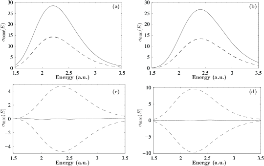
Figure 8: CO₂ results. The solid line is the sum from both channels, the dash lines are the two channel contributions. (a) ${\rm Re}[\sigma_{0000}^{(k)}(E)]=\sigma_{0000}^{(k)}(E)$; (b) ${\rm Re}[\sigma^{(k)}_{0101}(E)]=\sigma^{(k)}_{0101}(E)$; (c) Re[$\sigma^{(k)}_{0100}(E)$]; (d) Im[$\sigma^{(k)}_{0100}(E)$].

Figure 8 shows $\sigma_{0000}^{(r)}(E),\sigma_{0101}^{(r)}(E)$, and $\sigma_{0100}^{(r)}(E)$ for CO₂. In this case the diagonal cross sections are strictly real. The off-diagonal cross section $\sigma_{0100}^{(r)}(E)$ do contain an imaginary component in both channels, but they are seen to be equal and opposite in magnitude, verified by computing the total cross section which is again strictly real.

To test the utility of this approach on a system where the two channels are dissimilar, we consider CH₂BrI where channel 1 is CH₂Br + I and channel 2 is CH₂I + Br. The upper potential energy surface is given by AB01

$$V(r_{\rm CH_{2}-Br},r_{\rm CH_{2}-I}) = [V_{\rm I}(r_{\rm CH_{2}-I})+V^{\rm Morse}_{\rm CH_{2}-Br}(r_{\rm CH_{2}-Br})]f(x)+$$

$$\mbox{}[V_{\rm Br}(r_{\rm CH_{2}-Br})+V^{\rm Morse}_{\rm CH_{2}-I}(r_{\rm CH_{2}-I})](1-f(x))$$

where

$$V^{\rm Morse}_{\rm CH_{2}-Br}(r_{\rm CH_{2}-Br}) = D^{e}_{\rm CH_{2}-Br}\exp\left\{-\alpha_{\rm Br}(r_{\rm CH_{2}-Br}-r_{\rm CH_{2}-Br}^{e})\right\}$$ (61)

$$\times[\exp\left\{-\alpha_{\rm Br}(r_{\rm CH_{2}-Br}-r_{\rm CH_{2}-Br}^{e})\right\}-2]$$

$$V^{\rm Morse}_{\rm CH_{2}-I}(r_{\rm CH_{2}-I}) = D^{e}_{\rm CH_{2}-I}\exp\left\{-\alpha_{\rm I}(r_{\rm CH_{2}-I}-r_{\rm CH_{2}-I}^{e})\right\}$$ (62)

$$\times[\exp\left\{-\alpha_{\rm I}(r_{\rm CH_{2}-I}-r_{\rm CH_{2}-I}^{e})\right\}-2]$$

$$V_{\rm I}(r_{\rm CH_{2}-I}) = A_{\rm I}\exp\left\{-\beta_{\rm I}r_{\rm CH_{2}-I}\right\},$$ (63)

$$V_{\rm Br}(r_{\rm CH_{2}-Br}) = A_{\rm Br}\exp\left\{-\beta_{\rm Br}r_{\rm CH_{2}-Br}\right\},$$ (64)

$$f(x) = \frac{1}{1+\exp\left\{\alpha(x-0.5)\right\}},$$ (65)

$$x = \frac{r_{\rm CH_{2}-Br}}{r_{\rm CH_{2}-I}+r_{\rm CH_{2}-Br}}.$$ (66)

The parameters for this surface are: $\alpha=30$, $D^{e}_{\rm CH_{2}-Br}=0.1069$ a.u., $\alpha_{\rm Br}=0.9154$ (a.u.)^-1, $r_{\rm CH_{2}-Br}^{e}=3.6850$ a.u., $A_{\rm Br}=0.27$, $\beta_{\rm Br}=0.35$, $D^{e}_{\rm CH_{2}-I}=0.0874$ a.u., $\alpha_{\rm I}=0.87094$ (a.u.)^-1, $r_{\rm CH_{2}-I}^{e}=4.04326$ a.u., $A_{\rm I}=0.37$, $\beta_{\rm I}=0.3$.

The initial state is taken to be harmonic in normal mode coordinates. These coordinates, $q_{1},q_{2}$, are related to the bond length coordinates $r_{\rm CH_{2}-Br}$ and $r_{\rm CH_{2}-I}$ by

$$r_{\rm CH_{2}-Br}-\bar{r}_{\rm CH_{2}-Br} = c_{11}q_{1}+c_{21}q_{2}$$ (67)

$$r_{\rm CH_{2}-I}-\bar{r}_{\rm CH_{2}-I} = c_{12}q_{1}+c_{22}q_{2}$$ (68)

where $c_{11}=0.552747$; $c_{21}=1.09614$; $c_{12}=0.788417$; $c_{22}=-1.03893$; $\bar{r}_{\rm CH_{2}-Br}=r_{\rm CH_{2}-Br}^{e}$; $\bar{r}_{\rm CH_{2}-I}=r_{\rm CH_{2}-I}^{e}$. The parameters for this system are:

$$M_{1}=162614.16\mbox{ a.u.};\;M_{2}=27238.15\mbox{ a.u.},$$ (69)

$$\alpha_{1}=149.3978\mbox{ a.u.};\;\alpha_{2}=98.8412\mbox{ a.u.},$$ (70)

$$\hbar\omega_{1}=201.638\mbox{ cm}^{-1};\;\hbar\omega_{2}=796.43112\mbox{ cm}^{-1}.$$ (71)

Results for several cross sections and interference terms are shown in Figs. 9 to 11. The diagonal cross sections are strictly real. For this system, unlike CO₂, the real part of the channel specific results can be different in the two channels.

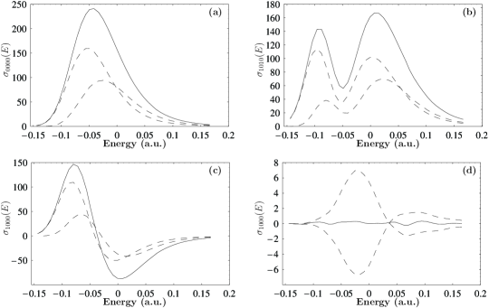
Figure 9: CH₂BrI results. The solid line is the sum from both channels, the dash lines are the two channel contributions. (a) ${\rm Re}[\sigma^{(k)}_{0000}(E)]=\sigma^{(k)}_{0000}(E)$; (b) ${\rm Re}[\sigma^{(k)}_{1010}(E)]=\sigma^{(k)}_{1010}(E)$; (c) Re[$\sigma^{(k)}_{1000}(E)$]; (d) Im[$\sigma^{(k)}_{1000}(E)$].

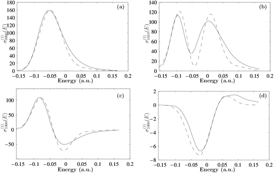
Figure 10: CH₂BrI results, comparing the Wigner-classical method (solid) to the quantum (dash) for the CH₂Br + I channel. (a) ${\rm Re}[\sigma^{(1)}_{0000}(E)]=\sigma^{(1)}_{0000}(E)$; (b) ${\rm Re}[\sigma^{(1)}_{1010}(E)]=\sigma^{(1)}_{0000}(E)$; (c) Re[$\sigma^{(1)}_{1000}(E)$]; (d) Im[$\sigma^{(1)}_{1000}(E)$].

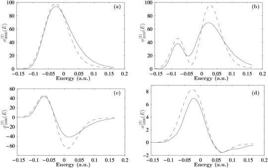
Figure 11: CH₂BrI results, comparing the Wigner-classical method (solid) to the quantum (dash) for the CH₂I + Br channel. (a) ${\rm Re}[\sigma^{(2)}_{0000}(E)]=\sigma^{(2)}_{0000}(E)$; (b) ${\rm Re}[\sigma^{(2)}_{1010}(E)]=\sigma^{(2)}_{1010}(E)$; (c) Re[$\sigma^{(2)}_{1000}(E)$]; (d) Im[$\sigma^{(2)}_{1000}(E)$].

Figure 9 shows the structure of the channel contributions to various cross sections and interference terms. Note that, as required, for the case of the off-diagonal cross section $\sigma_{1000}^{(k)}(E)$ is interesting (cf. Fig. 9 ), even though the two channels produce different real parts, the imaginary parts in the two channels again sum to zero. The deviation from zero is very small, indicating reliable convergence of the Monte Carlo sums.

Figures 10 and 11 show a comparison of the classical-Wigner method with a full quantum mechanical calculation. The structure of the cross section in the channels is seen to be well reproduced the classical-Wigner method, providing support for the conclusion that this approach gives reliable results for both the real and imaginary contribution. Interestingly, the latter arises via the non-Hermitian character of $\hat{R}_{r}\delta(E-\hat{H})$.

Finally, Fig. 12 shows an example of the utility of larger values of $\epsilon$ in Eq. (51). Specifically, using larger values of $\epsilon$ allows for a qualitative estimate of the desired integrals using far fewer trajectories.

Figure 12: CH₂BrI results for $\sigma_{0000}^{(1)}(E)$ (CH₂Br + I) with different $\epsilon$. Dash: $\epsilon=5\times 10^{-7}$, $2\times 10^{4}$ trajectories; Solid: $\epsilon=10^{-8}$, $10^{6}$ trajectories per energy.

VII SUMMARY

We have considered a Wigner-based classical approximation [Eq. (14)] to compute the terms $\sum_{r}\langle E,k^{-}|\mu_{fi}|n\rangle\langle m|\mu_{fi}|E,k^{-}\rangle$, with $n\neq m$, that are central to the interference contributions characteristic of coherent control. In the case of a single open product arrangement channel the accuracy of this formula for the Franck-Condon transitions onto a linear potential, along with the dependence of the method on parameters such as system reduced mass, slope of the upper potential energy surface, and vibrational frequency of the lower electronic state were examined. The results were found to be in excellent agreement when the newly introduced parameter $s_{n,m}$ [Eq. (33)] was less than unity. A comparison of the classical and uniform semiclassical approximations for the transitions between the realistic potential energy surfaces of Na₂ demonstrates that higher values of $m,n$ require use of the anharmonic Wigner function for the ground state, an effect not explored in this paper.

This approach was also applied to the multi-channel problem where interference terms are complex. In this case, the result is still the overlap of two time-independent phase space densities, but determining the density associated with a particular channel required evaluation using classical trajectories. The non-Hermitian character introduced by the projection operator $\hat{R}_{r}$ onto channel $r$ allowed for the successful reproduction of the entire complex term. We regard it as particularly encouraging that use of classical trajectories in conjunction with the complex Wigner transform of the term $|i\rangle\langle j|$ suffices to produce the imaginary part of the interference contribution with such accuracy. We note, however, that the method is not expected to produce resonance structures in the cross section, being most useful for systems where the dynamics is direct and short-livedHupper ; Hupper1 ; Miller2 .

Applications to full 3 dimensional photodissociation computations and to scattering (for bimolecular coherent controlcc ; bmcc are underway.

References

References

• (1) S. A. Rice and M. Zhao, Optical Control of Molecular Dynamics (Wiley, New York, 2000); M. Shapiro and P. Brumer, Adv. Atom. Mol. Optical Phys. 42, 287 (2000); M. Shapiro and P. Brumer, Principles of the Quantum Control of Molecular Processes (Wiley, New York, 2003).
• (2) V. S. Batista and P. Brumer, Phys. Rev. Lett. 89, 143201 (2002); J. Chem. Phys. 114, 10321 (2001); J. Phys. Chem. 105, 2591 (2001).
• (3) For a review see W. H. Miller, J. Phys. Chem. A105, 2942 (2001)
• (4) E. Wigner, Phys. Rev. 40, 749 (1932).
• (5) K. Imre, E. Ozizmir, M. Rosenbaum, and P.F. Zweifel, J. Math. Phys. 8, 1097 (1967).
• (6) E.J. Heller, J. Chem. Phys. 68, 2066 (1978). $\lambda=\omega$ in this reference should be $\lambda=2\omega$.
• (7) E. J. Heller and M. J. Davis, J. Chem. Phys. 84, 1999 (1980); H. W. Lee and M. O. Scully, J. Chem. Phys. 73, 2238 (1980); J. S. Hutchinson and R. E. Wyatt, Chem. Phys. Lett. 72, 384 (1990); M. Sizun and S. Goursaud, J. Chem. Phys. 71, 4042 (1979).
• (8) B. Hüpper and B. Eckhardt, Phys. Rev. A 57, 1536 (1998).
• (9) B. Hüpper and B. Eckhardt, J. Chem. Phys. 110, 11749 (1999).
• (10) C. Jaffe and P. Brumer, J. Chem. Phys. 82, 2330 (1985); C. Jaffe, S. Kanfer and P. Brumer, Phys. Rev. Lett. 54, 8 (1985); J. Wilkie and P. Brumer, Phys. Rev. A 55, 27 (1997); ibid., 55, 43 (1997); ibid., 61, 064101 (2000).
• (11) See reference 3 and, e.g., H. Wang, X. Sun and W.H. Miller, J. Chem. Phys. 108, 9726 (1998); X. Sun, H. Wang and W.H. Miller, J. Chem. Phys, 109, 7064 (1998); ibid., 109, 7064 (1998).
• (12) E.g., M. Shapiro and P. Brumer, Chem. Phys. Lett. 126, 541 (1986).
• (13) T. Seideman, M. Shapiro and P. Brumer, J. Chem. Phys. 90, 7132 (1989); J. L. Krause, M. Shapiro, and P. Brumer, J. Chem. Phys. 92, 1126 (1990); I. Levy, M. Shapiro, and P. Brumer, J. Chem. Phys. 93, 2493 (1990); D. G. Abrashkevich, M. Shapiro, and P. Brumer, J. Chem. Phys. 108, 3585 (1998).
• (14) D. Wardlaw, P. Brumer, and T. A. Osborn, J. Chem. Phys. 76, 4916 (1982).
• (15) J. E. Mayer and W. Band, J. Chem. Phys. 15, 141 (1947).
• (16) C. Jaffé and P.Brumer, J.Phys. Chem. 88, 4829 (1984). G.
• (17) Herzberg, Spectra of Diatomic Molecules (Van Nostrand, Princeton, N.J., 1950).
• (18) I. Schmidt, Ph.D. thesis, Kaiserslautern University, 1987.
• (19) B. R. Johnson, J. Chem. Phys., 67, 4086 (1977).
• (20) R. E. Langer, Phys. Rev. 51, 669 (1937).
• (21) W. H. Miller, J. Chem. Phys. 48, 464 (1968).
• (22) E. J. Heller and R. C. Brown, J. Chem. Phys. 75, 1048 (1981).
• (23) H. J. Groenewold, Physica 12, 405 (1946).
• (24) K. C. Kulander, C. Cerjan, and A. E. Orel, J. Chem. Phys. 94, 2571 (1991).
• (25) B. R. McQuarrie and P. Brumer, Chem. Phys. Lett. 319, 27 (2000).
• (26) D. G. Abrashkevich, M. Shapiro, and P. Brumer, J. Chem. Phys. 116, 5584, (2002).
• (27) W. H. Press, S. A. Teukolsky, W. T. Vetterling, and B. P. Flannery, Numerical Recipes: The Art of Scientific Computing, 2nd Ed. (Cambridge University Press, Cambridge, 1996).
• (28) See, e.g., A. Abrashkevich, M. Shapiro and P. Brumer, Chem. Phys. 267, 81 (2001)