Pole dynamics for the Flierl-Petviashvili equation and zonal flow

Abstract

We use a systematic method which allows us to identify a class of exact solutions of the Flierl-Petvishvili equation. The solutions are periodic and have one dimensional geometry. We examine the physical properties and find that these structures can have a significant effect on the zonal flow generation.

Keywords: Drift waves, Flierl-Petviashvili equation, pole dynamics, zonal flows.

1 Introduction

The problem of coherent structures has been extensively investigated in connection with the drift wave modes in tokamak. Numerical simulations and experimental observations have provided strong evidence of the presence of long-lived, cuasi-coherent structures even in deep turbulent regimes. The theoretical models (close to similar descriptions in the physics of fluids, atmosphere and ocean) emphasize the role of two types of nonlinearity : scalar (or Korteweg deVries-type) and vectorial (convection of the vorticity). Both are able to support vortical flow in a form of coherent and long lived structures. The problems of generation from initial conditions and the stability of monopolar or multipolar vortices are subjects of intense research and one of the notable result is that not all of these structures can be expected to be solitons in the sense of the Inverse Scattering Method. Usually they are called solitary waves or solitary vortices. A review, mainly oriented to plasma physics applications, has been done by Horton and Hasegawa [1].

The ion drift wave equation has a distinct dynamical character according to the space-time scales involved. For shorter scales the Hasegawa-Mima-Charney equation is obtained and the dynamics exhibits dipolar structures on the Larmor radius scale. On larger scales the scalar (or KdV-type) nonlinearity is prevailing and the structures are monopolar. Both are not solitonic but very robust and long lived. In the latter case the one-dimensional version of the equation can be reduced to the modified Korteweg De Vries (mKdV) equation [2] and has been derived in various contexts in plasma physics. Tasso [3] and later Petviashvili [4] have derived versions of this equations applicable to the case where there is a strong temperature gradient. It has been shown [5], [6] that the equation proposed was in fact exclusively dependent of the density gradient. Later the equation has been rederived along with a careful analysis of the scales involved [7], resolving a controversy on the role of the temperature gradient. In the study of ocean flows Flierl [8] has independently formulated an equation with the same structure. A one dimensional version of the equation has been solved by Lakhin et al. on an infinite domain [5], obtaining as solution the KdV soliton. The two dimensional case has been examined by Kadomtsev and Petviashvili [9] and by Petviashvili et al. [10] using trial functions to extremize a functional derived from the equation. The solution they found is vortical monopolar. Boyd and Tan [11] have found a monopolar solution expressed as a sum of $45$ terms depending on the radial coordinate $r$ through trigonometric functions. They have also proved the non-existence of stable non-axisymmetric solutions to the stationary Flierl-Petviashvili equation [12]. There is a strong connection between the stationary Flierl-Petviashvili equation and the Zakharov-Kuznetsov equation [13], a two-dimensional generalization of the KdV equation. This has also been investigated in Refs.[14] and [15] where multidimensional nonlinear wave structures (of the electrostatic drift wave branch) in inhomogeneous plasmas were studied by combining the eigenvalue problem in inhomogeneity and the $2D$ nonlinear vortex equation. For a two-dimensional generalization of the KdV equation numerical results are available [16]. For shorter reference it is used also the name Regularized Long Wave equation, RLW, since the equation proposed by Peregrine [17] can be brought to the same form.

The stationary two-dimensional equation derived in the studies mentioned above has a very simple structure. and a one-dimensional solution is known, the KdV soliton. We will examine the possible extension to an analytical closed form of a two dimensional solution. We are motivated by the studies of plasma ion mode instabilities, in particular the generation of radially localised layers of sheared flow (zonal flow).

2 Derivation of the equation

The ion instabilities are dominated by the nonlinearity related to the polarization drift. When the temperature gradient is very small the quasi-three dimensional geometry assumed in the derivation of the Haswgawa-Mima equation leads to suppression of the classical convection nonlinearity although the presence of the later can still be important in a fluctuation model. The ion polarisation drift nonlinearity may support vortical flows of which certain states are stable and coherent (actually not solitonic). The derivation of a nonlinear equation in this case starts by the ion density continuity

$$\left(\frac{\partial}{\partial t}+\mathbf{v}_{i\perp}\cdot\mathbf{\nabla}_{\perp}\right)n_{i}+n_{0}\left(\mathbf{\nabla}_{\perp}\cdot\mathbf{v}\right)=0$$ (1)

and assuming neutrality and adiabatic response of the particles

$$n_{i}\approx n_{e}\approx n_{0}\frac{e\varphi}{T_{e}}$$

The ion velocity in two dimension is

$$\mathbf{v}_{i\perp}=\frac{-\mathbf{\nabla}_{\perp}\varphi\times\widehat{\mathbf{n}}}{B}-\frac{1}{\Omega_{i}B}\left(\frac{\partial}{\partial t}+\frac{-\mathbf{\nabla}_{\perp}\varphi\times\widehat{\mathbf{n}}}{B}\cdot\mathbf{\nabla}_{\perp}\right)\mathbf{\nabla}_{\perp}\varphi$$ (2)

The Eqs.(1) and (2) lead to a nonlinear equation for the electrostatic potential. However, in these two equations there is still much freedom and a detailed analysis of the time and space scales leads to different particular forms of this equation. This is a multiple space and time scale analysis [23], [7], [24]

$$x_{i} = \varepsilon^{i}x$$

$$t_{i} = \varepsilon^{i}t$$

for $\varepsilon\ll 1$. It is possible to change to a moving frame, by introducing a translation velocity, $u$.

$$\eta=y-ut$$

The speed $u$ can also be a function on certain space and time scales.

We recall the main steps of the analysis performed in Ref. [7]. In the scaling

$$\varphi=\varepsilon\varphi_{1}+\varepsilon^{2}\varphi_{2}+\ldots$$

with

$$\varphi_{1}=\varphi_{1}\left(x_{0},x_{1},x_{2},...,\eta_{0},\eta_{1},\eta_{2},...,t_{0},t_{1},t_{2},...\right)$$

$$u\sim u_{1}\equiv O\left(\varepsilon\right)$$

$$n_{0}=n_{0}\left(x_{1},x_{2},...\right)$$

$$T_{e}=T_{e}\left(x_{1},x_{2},...\right)$$

In this scaling $n_{0}$ and $T_{e}$ have variations on only “large” space scales, and the potential (which is of $\varepsilon$ -small amplitude) varies on the small space scale, $x_{0}$ and slow time scale, $t_{0}$ and, of course, on higher scales. The characteristic space scale for the potential is then $\rho_{s}$ which is the spatial extension of the dipolar vortex. The normalisation of the parameters can be done according to these scales

$$\phi = \frac{e\varphi}{T_{0}}\;,\;T=\frac{T_{e}}{T_{0}}\;,\;v=\frac{v_{i\perp}}{c_{s}}$$

$$x^{\prime} = x/\rho_{s}\;,\;\eta^{\prime}=\eta/\rho_{s}\;,\;t^{\prime}=\Omega_{i}^{-1}t$$

and dropping the primes, one obtains

$$\frac{\partial}{\partial t_{1}}\left[\frac{1}{T\left(x_{1}\right)}-\mathbf{\nabla}_{\perp 0}^{2}\right]\phi_{1}$$

$$+u_{1}\frac{\partial}{\partial\eta_{1}}\mathbf{\nabla}_{\perp 0}^{2}\phi_{1}-u_{1}\left(\frac{1}{T\left(x_{1}\right)}+\frac{\kappa_{n}\left(x_{1}\right)}{u_{1}}\right)\frac{\partial}{\partial\eta_{0}}\phi_{1}$$

$$-\left[\left(-\mathbf{\nabla}_{\perp 0}\phi_{1}\times\widehat{\mathbf{n}}\right)\cdot\mathbf{\nabla}_{\perp 0}\right]\mathbf{\nabla}_{\perp 0}^{2}\phi_{1}$$

$$= 0$$

where

$$\kappa_{n}\equiv L_{n}^{-1}=\frac{1}{n_{0}}\frac{\partial n_{0}}{\partial x}$$

is varying on the larger space scale, $x_{1}$.

This is the Hasegawa-Mima equation governing the space variation of the potential $\phi_{1}$ on the smaller space scale, $x_{0}$ and $\eta_{0}$ of the order $\rho_{s}$ and on times of the scale $t_{1}$. On these scales several simplifications are obvious, since the temperature and the density gradient lengths can be taken constants

$$\kappa_{n}/u_{1} \sim \text{constant on }x_{0}$$

$$T \sim \text{constant on }x_{0}$$

A different dynamical equation is obtained on other space-time scale

$$\phi=\varepsilon^{2}\phi_{2}+\varepsilon^{3}\phi_{3}+...$$

$$\phi_{2}\equiv\phi_{2}\left(x_{1},x_{2},...,\eta_{1},\eta_{2},...,t_{5},t_{6},...\right)$$

$$n_{0}=n_{0}\left(x_{2},x_{3},...\right)$$

$$u=u_{2}\sim O\left(\varepsilon^{2}\right)$$

$$T=T\left(x_{2},x_{3},...\right)$$

The following combination has to be of a certain order in $\varepsilon$

$$\frac{1}{T\left(x_{2}\right)}+\frac{\kappa_{n}\left(x_{2}\right)}{u_{2}}\sim O\left(\varepsilon^{2}\right)$$

Then the equation on the time scale of order $5$ is

$$\frac{\partial}{\partial t_{5}}\frac{\phi_{2}}{T\left(x_{2}\right)}+u_{2}\frac{\partial}{\partial\eta_{1}}\mathbf{\nabla}_{\perp 1}^{2}\phi_{2}$$

$$-u_{2}\left[\frac{1}{T\left(x_{2}\right)}+\frac{\kappa_{n}\left(x_{2}\right)}{u_{2}}\right]\frac{\partial\phi_{2}}{\partial\eta_{1}}$$

$$+\kappa_{T}\left(x_{2}\right)\phi_{2}\frac{\partial\phi_{2}}{\partial\eta_{1}}$$

$$= 0$$

The operator of Laplacean in two dimension acts on the larger space scales

$$\mathbf{\nabla}_{\perp 1}^{2}\equiv\frac{\partial^{2}}{\partial x_{1}^{2}}+\frac{\partial^{2}}{\partial\eta_{1}^{2}}$$

The dominant space variation is here on the scale

$$x_{1}=\frac{\rho_{s}}{\varepsilon}$$

which is much larger than the dipolar vortex scale. The condition imposed by this ordering is

$$\kappa_{T}=\frac{\partial\kappa_{n}}{\partial x_{1}}\frac{1}{u_{2}}$$

In this range the nonlinear equation is dominated by the scalar nonlinearity. This equation leads, after one integration over the $\eta_{1}$ coordinate, to the Flierl-Petviashvili equation.

Spatschek et al. [7] also discuss intermediate scalings, where both the scalar and the vectorial nonlinearities are present. The stability analysis implies the concept of structural stability, where the dynamics governed by one of the equations obtained above (Hasegawa-Mima or scalar nonlinear) is perturbed with a term that is of the other type. It has been shown that the dipolar vortices are broken into separate monopolar vortices, while the monopolar vortices are structurally stable. To these consideration one should also add the numerical results from the collision of monopolar vortices of the Flierl-Petviashvili equation (or Zakharov-Kusnetsov) [11], [12], [16]. The monopolar vortices are stable and are not destroyed by collisions, however the form and the amplitides are perturbed, showing again that they are not exact solitons.

3 The scalar nonlinearity equation

In plasma physics applications, the Flierl-Petviashvili equation has the form

$$\Delta\phi=\alpha\phi-\beta\phi^{2}$$ (3)

where $\alpha$ and $\beta$ are physical parameters, i.e. functions depending on $\left(x,y\right)$. This equation is obtained as the stationary version of the equation which has been expressed in the system of reference moving with the velocity $u$

$$y\rightarrow y-ut$$

In the following, the coordinates $x$ and $y$ are the coordinates in the moving system. It is assumed that $y$ is the poloidal direction and $x$ is the radial direction in tokamak.

In the tokamak context the equation has been frequently simplified

$$\frac{\partial^{2}}{\partial x^{2}}\ll\frac{\partial^{2}}{\partial y^{2}}$$

leading to

$$\frac{\partial^{2}\phi}{\partial y^{2}}=\alpha\phi-\beta\phi^{2}$$ (4)

whose solution (Lakhin et al.[5]) is

$$\phi\left(x,y\right)=\frac{3\alpha/(2\beta)}{\cosh^{2}\left(\frac{\sqrt{\alpha}}{2}y\right)}$$ (5)

The dependence on $x$ is only parametric here, via the coefficients $\alpha$ and $\beta$. This has the same form as the KdV soliton solution.

Assuming that $\alpha$ and $\beta$ are constants, this solution can be extended indefinitely in the transversal ($x$) direction, as a ridge propagating in the $y$ direction whose section is given by Eq.(5). If the plasma is homogeneous, this ridge can be rotated arbitrarly in plane. We have then a family of quasi two dimensional solutions to the Eq.(3).

We will discuss the possibility to find other solutions of the two-dimensional version of the equation.

4 Starting from the one dimensional problem

We can directly integrate the one dimensional version of the equation (3). Actually, the solution (5) is one of the possible solutions arising from the direct integration. For a reason that will become clear later, we write the one dimensional version of the equation (3) in the form

$$\frac{d^{2}\phi}{d\left(i\eta\right)^{2}}=\alpha\phi-\beta\phi^{2}$$

where $i\eta$ can be $y$ as in Eq.(4). Multiplying by $d\phi/d\eta$ and integrating once we have

$$-\frac{1}{2}\left(\frac{d\phi}{d\eta}\right)^{2}=\frac{\alpha}{2}\phi^{2}-\frac{\beta}{3}\phi^{3}+\kappa$$

where $\kappa$ is a constant. Then we have the integral

$$\eta=\int^{\phi}\frac{d\phi}{\sqrt{\frac{2\beta}{3}\phi^{3}-\alpha\phi^{2}-2\kappa}}$$

The integral is elliptic and its inverse $\phi\left(\eta\right)$ has a closed analytical expression for all $\kappa$. Particular expressions can be written according to the reality of the roots of the third degree polynomial under the square root. For $\kappa$ such that all roots ($a>b>c$) are real, we have, for $\phi>a$

$$\int_{\phi}^{\infty}\frac{d\phi}{\sqrt{\left(\phi-a\right)\left(\phi-b\right)\left(\phi-c\right)}} = g\mathrm{sn}^{-1}\left(\sin\varphi,k\right)$$

$$= gF\left(\varphi,k\right)$$

where $\mathrm{sn}$ is the Jacobi elliptic sinus, $F$ is the incomplete elliptic integral of the first kind and the notations are

$$\varphi = \arcsin\sqrt{\frac{a-c}{\phi-c}}$$

$$g = \frac{2}{\sqrt{a-c}}$$

$$k^{2} = \frac{b-c}{a-c}$$

This expression can be easily inverted to obtain $\phi$ as function of $\eta$. An analoguous result is obtained when $\kappa$ is such that the root $a$ is real and $b$ and $c$ are complex. The integral is written, for $\phi>a$

$$\int_{\phi}^{\infty}\frac{d\phi}{\sqrt{\left(\phi-a\right)\left[\left(\phi-b_{1}\right)^{2}+a_{1}^{2}\right]}} = g\mathrm{cn}^{-1}\left(\cos\varphi,k\right)$$

$$= gF\left(\varphi,k\right)$$

where

$$b_{1} = \frac{\left(b+\overline{b}\right)}{2},\;a_{1}^{2}=-\frac{\left(b-\overline{b}\right)^{2}}{4}$$

$$g = \frac{1}{\sqrt{A}},\;A^{2}=\left(b_{1}-a\right)^{2}+a_{1}^{2}$$

$$k^{2} = \frac{A+b_{1}-a}{2A}$$

$$\varphi = \arccos\frac{\phi-a-A}{\phi-a+A}$$

Deatils on these Jacobian elliptic functions can be found in Ref.[18].

5 Constructing the solution from singularities

In view of the application to the description of plasma drift wave, a two-dimensional solution would be very useful. We already dispose of the one-parameter family of solutions with geometry of fronts, which has been obtained by simply translating a one-dimensional solution along the transversal direction. We examine a class of solutions that can be seen as an extension from the one-dimensional ones. We propose a more systematic approach of construction that makes more explicit the nature of the restriction leading to this quasi-one dimensional geometry.

We will start from the one dimensional model, taking the coefficients constants. The only analytical formula for a solution of (3) is [5]

$$\phi\left(y\right)=\phi_{0}\mathrm{sech}^{2}\left(\gamma y\right)$$

where

$$\phi_{0} = \frac{3\alpha}{2\beta}$$

$$\gamma = \frac{\sqrt{\alpha}}{2}$$

(note that in Lakhin et al. the coefficient must be corrected by dividing with $2$). We will use the following relation

$$\mathrm{sech}^{2}\left(z\right)=-\mathrm{cosech}^{2}\left(z-\frac{i\pi}{2}\right)$$

and the expression of the $\mathrm{cosech}$ function as a series using its pole singularities. Then we obtain

$$\phi\left(y\right)=\phi_{0}\mathrm{sech}^{2}\left(\gamma y\right)=-\phi_{0}\sum_{l=-\infty}^{\infty}\frac{1}{\left(\gamma y-\frac{i\pi}{2}+il\pi\right)^{2}}$$ (6)

We are looking for solutions $\phi\left(x,y\right)$ of the $2D$ equation and we try to build them from the motion of the pole singularities of the one-dimensional solution. More specifically, we will make an ansatz for the form of the $2D$ solution based on a particular choice of poles in the complex $y$ plane, as suggested by Eq.(6). We will assume that the poles have positions that depend on the other coordinate, $x$. Imposing that the function constructed in this way verifies the equation we obtain a set of differential equations and constraint conditions for the positions of the poles in the complex $y$ plane. The poles evolve with $x$ as time-like variable. Expressed in other terms, we look for a function that is meromorphic in the complex $y$ plane and whose poles depend on $x$. We find, following other similar approaches, that the solution is an elliptic function, i.e. a doubly periodic meromorphic function of $y$, for all values of $x$.

This procedure has been deveoped in the context of the exactly integrable differential equations like Kortweg de Vries. We follow closely the methods exposed in papers of Choodnovsky [20], Thickstun [21]. The work of Deconinck and Segur [22] is particularly relevant for our problem.

The following ansatz is suggested by the theory of $\tau$-functions in the integrable equations context [19]

$$\phi\left(x,y\right)=2\frac{\partial^{2}}{\partial y^{2}}\ln\tau\left(x,y\right)$$ (7)

where

$$\tau\left(x,y\right)=c\prod_{k=1}^{\infty}\left(1-\frac{y}{y_{k}}\right)\exp\left(\frac{y}{y_{k}}\right)$$ (8)

On the other hand, there is also the suggestion from Eq.(6) that the function $\phi$ is periodic on the imaginary $y$ axis. We choose a periodicity $iD$ (compare with $i\pi$ in the above equation) and take $N$ poles in each domain of periodicity. Then $\tau$ is

$$\tau\left(x,y\right)\sim c\prod_{n=1}^{N}\prod_{l=-\infty}^{\infty}\frac{1}{\left(y-y_{n}-ilD\right)^{2}}$$ (9)

We insert this expression in Eq.(7) and take care of the constants

$$\phi\left(x,y\right)=-2\phi_{0}\sum_{n=1}^{N}\sum_{l=-\infty}^{\infty}\frac{1}{\left[\gamma\left(y-y_{n}\right)-ilD\right]^{2}}$$ (10)

6 The dynamics of the singularities

6.1 Extending by inclusion of the $x$ coordinate

The $x$ dependence in this equation comes from the dependence on the variable $x$ of the position $y_{n}\left(x\right)$ of the poles in the complex $y$ plane. Now we impose that this form of $\phi$ verifies the equation.

$$\frac{\partial^{2}\phi}{\partial x^{2}}+\frac{\partial^{2}\phi}{\partial y^{2}}=\alpha\phi-\beta\phi^{2}$$

$$\frac{\partial\phi}{\partial x}=-4\gamma\phi_{0}\sum_{n=1}^{N}\sum_{l=-\infty}^{\infty}\left(\frac{dy_{n}\left(x\right)}{dx}\right)\frac{1}{\left[\gamma\left(y-y_{n}\right)-ilD\right]^{3}}$$

$$\frac{\partial^{2}\phi}{\partial x^{2}} = -4\gamma\phi_{0}\sum_{n=1}^{N}\sum_{l=-\infty}^{\infty}\left\{\frac{1}{\left[\gamma\left(y-y_{n}\right)-ilD\right]^{3}}\right.+$$

$$\left.+3\gamma\left(\frac{dy_{n}\left(x\right)}{dx}\right)^{2}\frac{1}{\left[\gamma\left(y-y_{n}\right)-ilD\right]^{4}}\right\}$$

$$\frac{\partial\phi}{\partial y}=4\gamma\phi_{0}\sum_{n=1}^{N}\sum_{l=-\infty}^{\infty}\frac{1}{\left[\gamma\left(y-y_{n}\right)-ilD\right]^{3}}$$

$$\frac{\partial^{2}\phi}{\partial y^{2}}=-12\gamma^{2}\phi_{0}\sum_{n=1}^{N}\sum_{l=-\infty}^{\infty}\frac{1}{\left[\gamma\left(y-y_{n}\right)-ilD\right]^{4}}$$

We replace these formulas and those for $\phi$ and $\phi^{2}$ in the equation. We will examine the neighborhood of one of the poles, taking

$$y=y_{p}\left(x\right)+\varepsilon$$

where $\varepsilon$ is a small quantity and $p$ is one of the $N$ poles . Expanding all terms in the equation in $\varepsilon$ we equal to zero the coefficients of the same powers of $\varepsilon$. This will give us the equations we have to impose to $y_{n}\left(x\right)$.

We have, with $\varepsilon\rightarrow 0$,

$$\phi = \frac{\left(-2\phi_{0}\right)}{\gamma^{2}}\frac{1}{\varepsilon^{2}}+$$

$$+\left(-2\phi_{0}\right)\sum_{\begin{subarray}{c}l=-\infty\\ l\neq 0\end{subarray}}^{\infty}\frac{1}{\left(-ilD\right)^{2}}+\left(-2\phi_{0}\right)\sum_{\begin{subarray}{c}n=1\\ n\neq p\end{subarray}}^{N}\sum_{l=-\infty}^{\infty}\frac{1}{\left[\gamma\left(y_{p}-y_{n}\right)-ilD\right]^{2}}$$

$$\frac{\partial^{2}\phi}{\partial x^{2}} = \left(-4\phi_{0}\gamma\right)\left(\frac{d^{2}y_{p}\left(x\right)}{dx^{2}}\right)\frac{1}{\gamma^{3}\varepsilon^{3}}+$$

$$+\left(-4\phi_{0}\gamma\right)\left(\frac{d^{2}y_{p}\left(x\right)}{dx^{2}}\right)\sum_{\begin{subarray}{c}l=-\infty\\ l\neq 0\end{subarray}}^{\infty}\frac{1}{\left(-ilD\right)^{3}}+$$

$$+\left(-4\phi_{0}\gamma\right)\sum_{\begin{subarray}{c}n=1\\ n\neq p\end{subarray}}^{N}\left(\frac{d^{2}y_{n}\left(x\right)}{dx^{2}}\right)\sum_{l=-\infty}^{\infty}\frac{1}{\left[\gamma\left(y_{p}-y_{n}\right)-ilD\right]^{3}}+$$

$$+\left(-12\phi_{0}\gamma^{2}\right)\left(\frac{dy_{p}\left(x\right)}{dx}\right)^{2}\frac{1}{\gamma^{4}\varepsilon^{4}}+$$

$$+\left(-12\phi_{0}\gamma^{2}\right)\left(\frac{dy_{p}\left(x\right)}{dx}\right)^{2}\sum_{\begin{subarray}{c}l=-\infty\\ l\neq 0\end{subarray}}^{\infty}\frac{1}{\left(-ilD\right)^{4}}+$$

$$+\left(-12\phi_{0}\gamma^{2}\right)\sum_{\begin{subarray}{c}n=1\\ n\neq p\end{subarray}}^{N}\left(\frac{dy_{n}\left(x\right)}{dx}\right)^{2}\sum_{l=-\infty}^{\infty}\frac{1}{\left[\gamma\left(y_{p}-y_{n}\right)-ilD\right]^{4}}$$

$$\frac{\partial^{2}\phi}{\partial y^{2}} = \left(-12\phi_{0}\gamma^{2}\right)\frac{1}{\gamma^{4}\varepsilon^{4}}+$$

$$+\left(-12\phi_{0}\gamma^{2}\right)\sum_{\begin{subarray}{c}l=-\infty\\ l\neq 0\end{subarray}}^{\infty}\frac{1}{\left(-ilD\right)^{4}}+$$

$$+\left(-12\phi_{0}\gamma^{2}\right)\sum_{\begin{subarray}{c}n=1\\ n\neq p\end{subarray}}^{N}\sum_{l=-\infty}^{\infty}\frac{1}{\left[\gamma\left(y_{p}-y_{n}\right)-ilD\right]^{4}}$$

$$\phi^{2} = 4\phi_{0}^{2}\left\{\frac{1}{\gamma^{4}\varepsilon^{4}}\right.+$$

$$+\frac{1}{\gamma^{2}\varepsilon^{2}}\left[2\sum_{\begin{subarray}{c}l=-\infty\\ l\neq 0\end{subarray}}^{\infty}\frac{1}{\left(-ilD\right)^{2}}+2\sum_{\begin{subarray}{c}n=1\\ n\neq p\end{subarray}}^{N}\sum_{l=-\infty}^{\infty}\frac{1}{\left[\gamma\left(y_{p}-y_{n}\right)-ilD\right]^{2}}\right]+$$

$$\left.+\left[\sum_{\begin{subarray}{c}l=-\infty\\ l\neq 0\end{subarray}}^{\infty}\frac{1}{\left(-ilD\right)^{2}}+\sum_{\begin{subarray}{c}n=1\\ n\neq p\end{subarray}}^{N}\sum_{l=-\infty}^{\infty}\frac{1}{\left[\gamma\left(y_{p}-y_{n}\right)-ilD\right]^{2}}\right]^{2}\right\}$$

We have to collect the terms containing the same powers of $\varepsilon$, begining with the highest. For easy identification, we show separately the contributions of each term of the original equation.

For $1/\varepsilon^{4}$:

$$\left(-12\phi_{0}\gamma^{2}\right)\left(\frac{dy_{p}\left(x\right)}{dx}\right)^{2}\frac{1}{\gamma^{4}\varepsilon^{4}}+$$

$$\left(-12\phi_{0}\gamma^{2}\right)\frac{1}{\gamma^{4}\varepsilon^{4}}+$$

$$\left(-\alpha\right)\times 0+$$

$$\beta 4\phi_{0}^{2}\frac{1}{\gamma^{4}\varepsilon^{4}}$$

$$= 0$$

This gives the equation

$$\left(\frac{dy_{p}\left(x\right)}{dx}\right)^{2}=\frac{1}{3}\frac{\phi_{0}\beta}{\gamma^{2}}-1$$ (11)

or

$$\left(\frac{dy_{p}\left(x\right)}{dx}\right)^{2}=1$$ (12)

For $1/\varepsilon^{3}$:

$$\left(-4\phi_{0}\gamma\right)\left(\frac{d^{2}y_{p}\left(x\right)}{dx^{2}}\right)\frac{1}{\gamma^{3}\varepsilon^{3}}+$$

$$0+$$

$$\left(-\alpha\right)\times 0+$$

$$\beta\times 0$$

$$= 0$$

The resulting equation is

$$\frac{d^{2}y_{p}\left(x\right)}{dx^{2}}=0$$ (13)

Finally, the coefficient of $1/\varepsilon^{2}$:

$$0+$$

$$0+$$

$$\left(-\alpha\right)\times\frac{\left(-2\phi_{0}\right)}{\gamma^{2}}\frac{1}{\varepsilon^{2}}+$$

$$\beta\times 4\phi_{0}^{2}\frac{1}{\gamma^{2}\varepsilon^{2}}\left[2\sum_{\begin{subarray}{c}l=-\infty\\ l\neq 0\end{subarray}}^{\infty}\frac{1}{\left(-ilD\right)^{2}}+2\sum_{\begin{subarray}{c}n=1\\ n\neq p\end{subarray}}^{N}\sum_{l=-\infty}^{\infty}\frac{1}{\left[\gamma\left(y_{p}-y_{n}\right)-ilD\right]^{2}}\right]$$

$$= 0$$

This results in the following constraint

$$\sum_{\begin{subarray}{c}l=-\infty\\ l\neq 0\end{subarray}}^{\infty}\frac{1}{\left(-ilD\right)^{2}}+\sum_{\begin{subarray}{c}n=1\\ n\neq p\end{subarray}}^{N}\sum_{l=-\infty}^{\infty}\frac{1}{\left[\gamma\left(y_{p}-y_{n}\right)-ilD\right]^{2}} = -\frac{\alpha}{2\phi_{0}\beta}$$

$$= -\frac{1}{3}$$

From the Eqs.(13) and (12) it results that the “trajectories”  $y_{p}\left(x\right)$ are linear on $x$. We have

$$\frac{dy_{p}\left(x\right)}{dx}=\pm 1$$ (15)

or

$$y_{p}\left(x\right)=\pm x+c_{p}$$ (16)

where $c_{p}$ are constants.

6.2 Discussion of the constraint equation

We have obtained the equations and the constraint using an expansion around a singularity $y_{p}$. The choice is arbitrary and we can repeat the calculations using another singularity. Obviously, the form of the equations will not be changed. Finally, we will obtain a number of constraints equal to the number of singularities.

A simpler form of the constraint can be written.

$$\sum_{\begin{subarray}{c}l=-\infty\\ l\neq 0\end{subarray}}^{\infty}\frac{1}{\left(-ilD\right)^{2}}=\frac{1}{\left(-iD\right)^{2}}2\sum_{l=1}^{\infty}\frac{1}{l^{2}}=-\frac{\pi^{2}}{3D^{2}}$$

We introduce the notation

$$z_{pn}\equiv\frac{i\gamma}{D}\left(y_{p}-y_{n}\right)$$

and we have

$$-\frac{1}{D^{2}}\sum_{\begin{subarray}{c}n=1\\ n\neq p\end{subarray}}^{N}\sum_{l=-\infty}^{\infty}\frac{1}{\left(z_{pn}+l\right)^{2}}=\frac{\pi^{2}}{3D^{2}}-\frac{1}{3}$$

The second sum can be written

$$\sum_{l=-\infty}^{\infty}\frac{1}{\left(z_{pn}+l\right)^{2}}=-\frac{1}{z_{pn}^{2}}+\psi^{\prime}\left(z_{pn}\right)+\psi^{\prime}\left(-z_{pn}\right)$$

and the constraints become, for $p=1,...,N$

$$\sum_{\begin{subarray}{c}n=1\\ n\neq p\end{subarray}}^{N}\left[\frac{D^{2}}{\gamma^{2}\left(y_{p}-y_{n}\right)^{2}}+\psi^{\prime}\left(\frac{y_{p}-y_{n}}{iD/\gamma}\right)+\psi^{\prime}\left(\frac{y_{n}-y_{p}}{iD/\gamma}\right)\right]=-\frac{\pi^{2}-D^{2}}{3}$$

In these formulas, $\psi^{\prime}$ is the first derivative of the Euler psi-function. This form can be useful if one wants to examine numerically the validity of a particular choice of constants $c_{p}$.

Alternatively we can use the expansion for the square of the $\mathrm{cosech}$ function, as before.

$$\sum_{l=-\infty}^{\infty}\frac{1}{\left[\gamma\left(y_{p}-y_{n}\right)-ilD\right]^{2}}=\frac{\pi^{2}}{D^{2}}\mathrm{cosech}^{2}\left[\frac{\pi\gamma}{D}\left(y_{p}-y_{n}\right)\right]$$

and the form of the constraint becomes

$$\frac{\pi^{2}}{D^{2}}\sum_{\begin{subarray}{c}n=1\\ n\neq p\end{subarray}}^{N}\mathrm{cosech}^{2}\left[\frac{\pi\gamma}{D}\left(y_{p}-y_{n}\right)\right]=\frac{\pi^{2}}{3D^{2}}-\frac{1}{3}$$ (17)

The following identity exists

$$\sum_{k=1}^{s-1}\mathrm{cosec}^{2}\left(\frac{k\pi}{s}\right)=\frac{s^{2}-1}{3}$$ (18)

Comparing our equation with the identity and using the elementary relation

$$\mathrm{cosech}^{2}\left(ix\right)=-\mathrm{cosec}^{2}\left(x\right)$$

it is suggested to identify

$$s\equiv\frac{D}{\pi}$$ (19)

$$\gamma\left(y_{p}-y_{n}\right)/i=k\pi$$ (20)

At this moment the solution can be written

$$\phi\left(x,y\right) = -2\phi_{0}\sum_{n=1}^{N}\sum_{l=-\infty}^{\infty}\frac{1}{\left[\gamma\left(y-y_{n}\right)-ilD\right]^{2}}$$

$$= -2\phi_{0}\frac{\pi^{2}}{D^{2}}\sum_{n=1}^{N}\mathrm{cosech}^{2}\left[\frac{\pi\gamma}{D}\left(y\pm x+c_{n}\right)\right]$$

Regarding the determination of the constants $c_{p}$, $p=1,...,N$ we note that the condition (20) only says that the differences between the values must be a multiple of $\pi i$. However, there is the additional constraint that the constants cannot vanish. This is because the function would present singularities in the real space variable. On the other hand, the singularities must be placed symmetrically along the imaginary axis. These makes three restriction to any choice of the constants of integration

1. the initial constraint, Eq.(17) which has been trasformed into Eq.(20)

2. the restriction $c_{p}\neq 0$

3. the symmetrical positions along the imaginary axis, in order to have real solutions.

This leads to the following choice

$$\gamma c_{k}=k\pi i+\frac{i\pi}{2}$$

where $k=-N,...,N$.

We will assume in the following that the number of poles is infinite,

$$N\rightarrow\infty$$

However this will be discussed in more detail below.

The problem of ennumeration of poles with $\pm x$ is so suppressed but we will have to make all steps separately for the two $\pm$ families. The fact that we can choose only two families is related to the impossibility to satisfy the constraints in the case when we would choose arbitrary combinations of the sign of $x$’s in $\left(y_{p}-y_{n}\right)$.

The constraints become two infinite systems of equations implying only $c_{k}$, the constants. Then the solution can be written

$$\phi\left(x,y\right) = -2\phi_{0}\frac{\pi^{2}}{D^{2}}\sum_{n=1}^{\infty}\mathrm{cosech}^{2}\left[\frac{\pi\gamma}{D}\left(y+x+c_{n}\right)\right]+$$

$$-2\phi_{0}\frac{\pi^{2}}{D^{2}}\sum_{n=1}^{\infty}\mathrm{cosech}^{2}\left[\frac{\pi\gamma}{D}\left(y-x+c_{n}^{\prime}\right)\right]$$

We can add to this expression the constraint equation, multiplied with $\left(2\phi_{0}\right)$ and written as an identity with zero.

$$\phi\left(x,y\right) =$$

$$-2\phi_{0}\frac{\pi^{2}}{D^{2}}\sum_{n=1}^{\infty}\mathrm{cosech}^{2}\left[\frac{\pi\gamma}{D}\left(y+x+c_{n}\right)\right]+$$

$$+\left(2\phi_{0}\right)\frac{\pi^{2}}{D^{2}}\sum_{n=1}^{\infty}\mathrm{cosech}^{2}\left[\frac{\pi\gamma}{D}\left(c_{p}-c_{n}\right)\right]-\left(2\phi_{0}\right)\left(\frac{\pi^{2}}{3D^{2}}-\frac{1}{3}\right)$$

$$-2\phi_{0}\frac{\pi^{2}}{D^{2}}\sum_{n=1}^{\infty}\mathrm{cosech}^{2}\left[\frac{\pi\gamma}{D}\left(y-x+c_{n}^{\prime}\right)\right]$$

$$+\left(2\phi_{0}\right)\frac{\pi^{2}}{D^{2}}\sum_{n=1}^{\infty}\mathrm{cosech}^{2}\left[\frac{\pi\gamma}{D}\left(c_{p}^{\prime}-c_{n}^{\prime}\right)\right]-\left(2\phi_{0}\right)\left(\frac{\pi^{2}}{3D^{2}}-\frac{1}{3}\right)$$

If the constants are chosen as suggested before then we have to exclude from the sum the term corresponding to $n=0$.

$$\phi\left(x,y\right) =$$

$$-2\phi_{0}\frac{\pi^{2}}{D^{2}}\sum_{\begin{subarray}{c}n=-\infty\\ n\neq 0\end{subarray}}^{\infty}\left\{\mathrm{cosech}^{2}\left[\frac{\pi\gamma}{D}\left(y+x+\frac{i\pi}{2\gamma}+\frac{n\pi i}{\gamma}\right)\right]-\mathrm{cosech}^{2}\left[\frac{\pi}{D}n\pi i\right]\right\}$$

$$-\left(2\phi_{0}\right)\left(\frac{\pi^{2}}{3D^{2}}-\frac{1}{3}\right)-2\phi_{0}\frac{\pi^{2}}{D^{2}}\mathrm{cosech}^{2}\left[\frac{\pi\gamma}{D}\left(y+x+\frac{i\pi}{2\gamma}\right)\right]$$

$$-2\phi_{0}\frac{\pi^{2}}{D^{2}}\sum_{\begin{subarray}{c}n=-\infty\\ n\neq 0\end{subarray}}^{\infty}\left\{\mathrm{cosech}^{2}\left[\frac{\pi\gamma}{D}\left(y-x+\frac{i\pi}{2\gamma}+\frac{n\pi i}{\gamma}\right)\right]-\mathrm{cosech}^{2}\left[\frac{\pi}{D}n\pi i\right]\right\}$$

$$-\left(2\phi_{0}\right)\left(\frac{\pi^{2}}{3D^{2}}-\frac{1}{3}\right)-2\phi_{0}\frac{\pi^{2}}{D^{2}}\mathrm{cosech}^{2}\left[\frac{\pi\gamma}{D}\left(y-x+\frac{i\pi}{2\gamma}\right)\right]$$

For a reason that will become clear later we can only chose the positive sign of $i\pi/2$.

This can further be written

$$\phi\left(x,y\right) =$$

$$-2\phi_{0}\frac{\pi^{2}}{D^{2}}\left(\frac{1}{3}+\sum_{\begin{subarray}{c}n=-\infty\\ n\neq 0\end{subarray}}^{\infty}\left\{\mathrm{cosech}^{2}\left[\frac{\pi\gamma}{D}\left(y+x+\frac{i\pi}{2\gamma}+\frac{n\pi i}{\gamma}\right)\right]-\mathrm{cosech}^{2}\left[\frac{\pi}{D}n\pi i\right]\right\}\right)$$

$$-2\phi_{0}\frac{\pi^{2}}{D^{2}}\mathrm{cosech}^{2}\left[\frac{\pi\gamma}{D}\left(y+x+\frac{i\pi}{2\gamma}\right)\right]$$

$$-2\phi_{0}\frac{\pi^{2}}{D^{2}}\left(\frac{1}{3}+\sum_{\begin{subarray}{c}n=-\infty\\ n\neq 0\end{subarray}}^{\infty}\left\{\mathrm{cosech}^{2}\left[\frac{\pi\gamma}{D}\left(y-x+\frac{i\pi}{2\gamma}+\frac{n\pi i}{\gamma}\right)\right]-\mathrm{cosech}^{2}\left[\frac{\pi}{D}n\pi i\right]\right\}\right)$$

$$-2\phi_{0}\frac{\pi^{2}}{D^{2}}\mathrm{cosech}^{2}\left[\frac{\pi\gamma}{D}\left(y-x+\frac{i\pi}{2\gamma}\right)\right]$$

$$+\frac{4}{3}\phi_{0}$$

Now we have to recall the identity for the doubly periodic elliptic Weierstrass function $\wp$

$$\frac{1}{3}+\mathrm{cosech}^{2}\left(\frac{\pi w}{L_{2}}\right)+$$

$$+\sum_{\begin{subarray}{c}n=-\infty\\ n\neq 0\end{subarray}}^{\infty}\left\{\mathrm{cosech}^{2}\left[\frac{\pi}{L_{2}}\left(w+nL_{1}\right)\right]-\mathrm{cosech}^{2}\left[\frac{n\pi L_{1}}{L_{2}}\right]\right\}$$

$$= \wp\left(w\right)\left(\frac{L_{2}}{\pi}\right)^{2}$$

Where $L_{1}$ and $L_{2}$ are respectively the period on the real axis and the period on the imaginary axis of the argument of $\wp$: $2\omega_{1}=L_{1}$ and $2\omega_{2}=iL_{2}$. We can identify

$$L_{1} = \pi i$$

$$L_{2} = D$$

and the two variables

$$w = \gamma\left(y+x\right)+\frac{i\pi}{2}$$ (22)

$$\text{or}\;w = \gamma\left(y-x\right)+\frac{i\pi}{2}$$

At this moment an important comment should be done. As we have seen the solution of the constraint equation can be obtained on the basis of the comparison with the identity Eq.(18). We observe that the upper limit of the summation in (18) is interpreted as the number of poles,

$$s-1=N$$

On the other hand we were led to identify

$$s=\frac{D}{\pi}$$

which means that the number of poles is the integer part

$$N=\left[\frac{D}{\pi}\right]+1$$

Since we consider an infinite number of poles, $N\rightarrow\infty$, this means that $D$ is infinite. This is necessary since we later use the identity (6.2) where the summation is extended over an infinite number of integer values $n$. Since however we find that $L_{2}=D$, this implies that the period $L_{2}$ of the Weierstrass function $\wp$ is infinite. Certainly this is not acceptable in this particular approach, (but in general it is meaningful) and this shows that the identification using Eq.(6.2) can only be an approximation. This also means that the solution can only be approximative. However, if we decide to use this approximative identification, we have to understand in what consists this approximation and where we can expect to intervene the error we have introduced by that.

We first note that the number of terms which is required in (6.2) to obtain a good approximation of the Weierstrass function is not necessarly large, for a significant area in the perodicity parallelogram of the complex argument. This means that actually $D$ can be taken finite and in this case the use of Eq.(18) becomes legitimate. What is the number of poles, $N$ and accordingly the length of periodicity $L_{1}=D$ in a reasonable approximation? From numerical experience it may be accepted that about five terms in the summation determining the Weierstrass function gives a reasonable result. Then the number of poles retained in the sums (i.e. $s-1=N$) can be a few units and this also means that $D\sim$few units.

In the following we will write the solution as being expressed in terms of the Weierstrass function, but we have to remember that it is the result of an approximation. It can be written

$$\phi\left(x,y\right) = \frac{4}{3}\phi_{0}$$

$$-2\phi_{0}\frac{\pi^{2}}{D^{2}}\wp\left[\gamma\left(x+y\right)+\frac{i\pi}{2}\right]\left(\frac{D}{\pi}\right)^{2}$$

$$-2\phi_{0}\frac{\pi^{2}}{D^{2}}\wp\left[\gamma\left(x-y\right)+\frac{i\pi}{2}\right]\left(\frac{D}{\pi}\right)^{2}$$

or

$$\phi\left(x,y\right)=\frac{4}{3}\phi_{0}-2\phi_{0}\left\{\wp\left[\gamma\left(x+y\right)+\frac{i\pi}{2}\right]+\wp\left[\gamma\left(x-y\right)+\frac{i\pi}{2}\right]\right\}$$ (23)

This expression represents in plane a system of rectangular cells.

We will prove later that a single family of poles corresponding to one of the two possibilities $\pm x$ in Eq.(16) , which generates either the first or the second term in the Eq.(23) can provide an exact solution to the equation. This justifies the calculations presented in this section, since after them we are led directly to the form of the solution.

7 The rôle of the elliptic function

7.1 Basic information on the Weierstrass elliptic function (lemniscate type)

The most important consequence of the calculations that have been presented is the generation of a periodic solution and the confirmation, by the method of motion of poles, of the class of quasi-one-dimensional solutions. In the absence of a systematic integration procedure (like Inverse Scattering Transform) we can be at least sure that this class represents a significant part of the space of solutions.

Even if Eq.(23) is the result of an approximation, it clearly shows that the solution should be searched in a form of a double periodic elliptic Weierstrass function. This function has appeared in our calculations independently of any attempt to integrate a one-dimensional version of the equation.

We note that

$$\frac{\partial^{2}}{\partial x^{2}}\wp\left[\gamma\left(x+y\right)+\frac{i\pi}{2}\right] = 6\gamma^{2}\left(\wp\left[\gamma\left(x+y\right)+\frac{i\pi}{2}\right]\right)^{2}-\frac{g_{2}}{2}$$

$$= \frac{\partial^{2}}{\partial y^{2}}\wp\left[\gamma\left(x+y\right)+\frac{i\pi}{2}\right]$$

Here $g_{2}$ is the second coefficient in the standard expression for the definition of the Weierstrass function

$$\wp^{-1}\left(y\right)\equiv u=\int_{y}^{\infty}\frac{dt}{\sqrt{4t^{3}-g_{2}t-g_{3}}}$$

In the following we will use this information to derive an exact solution of the Petviashvilli equation

$$\Delta\phi=\alpha\phi-\beta\phi^{2}$$ (24)

We start by a linear substitution

$$\phi\left(x,y\right)=s\psi\left(x,y\right)+\frac{\alpha}{2\beta}$$ (25)

(where $s$ is a constant) which transform the equation into

$$\Delta\psi=-s\beta\psi^{2}+\frac{\alpha^{2}}{4s\beta}-\frac{1}{s}\Delta\left(\frac{\alpha}{2\beta}\right)$$ (26)

We have allowed formally the space variation of the coefficients. For an easier reference to the properties of the Weierstrass function, we make a change of variables

$$x \rightarrow x_{c}=ix$$ (27)

$$y \rightarrow y_{c}=iy$$

which gives

$$\Delta_{c}\psi\left(x_{c},y_{c}\right)=s\beta\psi\left(x_{c},y_{c}\right)-\frac{\alpha^{2}}{4s\beta}+\frac{1}{s}\Delta\left(\frac{\alpha}{2\beta}\right)$$ (28)

We look for a solution having the dependence on the coordinates $x$ and $y$ mediated by a new function, which we denote by $u\left(x_{c},y_{c}\right)$

$$\psi\equiv\psi\left(u\right)$$ (29)

with

$$u\equiv u\left(x_{c},y_{c}\right)$$ (30)

and now we proceed to express the equation (28) using this form.

$$\frac{\partial\psi}{\partial x_{c}} = \frac{d\psi}{du}\frac{\partial u}{\partial x_{c}}$$

$$\frac{\partial^{2}\psi}{\partial x_{c}^{2}} = \frac{d^{2}\psi}{du^{2}}\left(\frac{\partial u}{\partial x_{c}}\right)^{2}+\frac{d\psi}{du}\frac{\partial^{2}u}{\partial x_{c}^{2}}$$

and analogous for $y$.

$$\Delta_{c}\psi\left(x_{c},y_{c}\right) = \frac{d^{2}\psi}{du^{2}}\left[\left(\frac{\partial u}{\partial x_{c}}\right)^{2}+\left(\frac{\partial u}{\partial y_{c}}\right)^{2}\right]$$

$$+\frac{d\psi}{du}\left[\Delta_{c}u\right]$$

$$= s\beta\psi^{2}-\frac{\alpha^{2}}{4s\beta}+\frac{1}{s}\Delta\left(\frac{\alpha}{2\beta}\right)$$

Suppose we find a function $u\left(x_{c},y_{c}\right)$ verifying the conditions

$$\Delta_{c}u = 0$$ (31)

$$\left(\frac{\partial u}{\partial x_{c}}\right)^{2}+\left(\frac{\partial u}{\partial y_{c}}\right)^{2} = q$$

where $q$ is a constant. In this case the equation could be written

$$\frac{d^{2}\psi}{du^{2}}=\frac{s\beta}{q}\psi^{2}-\frac{\alpha^{2}}{4s\beta q}+\frac{1}{qs}\Delta\left(\frac{\alpha}{2\beta}\right)$$ (32)

and this form has a known solution, from the identifications

$$\psi\left(u\right) \equiv \wp\left(u\right)$$ (33)

$$\frac{s\beta}{q} = 6$$

$$\frac{\alpha^{2}}{4s\beta q}-\frac{1}{qs}\Delta\left(\frac{\alpha}{2\beta}\right) = \frac{g_{2}}{2}$$

This is because we have the known relationship for the Weierstrass function

$$\frac{d^{2}\wp\left(u\right)}{du^{2}}=6\wp^{2}\left(u\right)-\frac{g_{2}}{2}$$ (34)

which has exactly the same form as (32). We find from Eq.(33)

$$q=\frac{s\beta}{6}$$ (35)

$$g_{2}=\frac{3\alpha^{2}}{\left(s\beta\right)^{2}}-\frac{6}{s^{2}\beta}\Delta\left(\frac{\alpha}{\beta}\right)$$ (36)

8 Exact periodic solution of the Flierl-Petviashvilli equation

We now turn to the solutions of the constraint equations defining $u$. It is clear that we may chose

$$u\left(x_{c},y_{c}\right)=ay_{c}+bx_{c}+\tau$$ (37)

where $a$, $b$ and $\tau$ can be complex. The following condition results

$$a^{2}+b^{2}=\frac{s\beta}{6}$$

In addition, a choice of $a$ and $b$ real numbers, which makes the first two terms in (37) purely imaginary, should be coroborated with the suggestion from Eq.(22) where the poles resulted shifted with a symmetric quantity with respect to the real axis. This time, due to the change of variables (27) everything is rotated. This yields the choice for $\tau$ as half of the period $\left(2\omega\right)$ on the real axis

$$\tau=\frac{\left(2\omega\right)}{2}$$

and the final form of the solution to the equation (24)

$$\phi\left(x,y\right)=\frac{\alpha}{2\beta}+s\wp\left(iay+ibx+\omega|g_{2}=\frac{3\alpha^{2}}{\left(s\beta\right)^{2}}+\frac{6}{s^{2}\beta}\Delta\left(\frac{\alpha}{\beta}\right),g_{3}\right)$$

The second Weierstrass coefficient $g_{3}$ is left unspecified but it must be constant.

We conclude that an exact solution to the Petviashvilli equation with constant coefficients $\alpha$ and $\beta$ is

$$\phi\left(x,y\right)=\frac{\alpha}{2\beta}+s\wp\left(iay+ibx+\omega|g_{2}=\frac{3\alpha^{2}}{\left(s\beta\right)^{2}}\right)$$ (38)

with the condition

$$a^{2}+b^{2}=\frac{s\beta}{6}$$ (39)

Now we understand the nature of the choice which is implicitely done when we discuss the solutions consisting of arbitrarly rotated ridges issued by translating one-dimensional profiles. It means to remain in the class of functions $u$ whose Laplacean is zero and the gradient is constant, according to the conditions (31). Or, it can easily be seen that the only functions that verify these conditions have the form of linear combinations of the variables $x$ and $y$.

9 The physical relevance of this periodic solution

As a mathematical result, Eq.(38) is the exact response to the problem of solving the Eq.(3). This is valid for any sign of $\alpha$ and $\beta$ since the function $\wp$ is doubly periodic. The physical problem, as usual, is more complicated. The coefficients $\alpha$ and $\beta$ which we have assumed constants actually have a certain space variation. We think however that it is worth examining the consequences of this solution for the nonlinear plasma models.

In order to discuss possible physical applications of this solution we have to handle easily its numerical form. Although we have assumed that the two parameters $\alpha$ and $\beta$ are constants, we will make estimations on the base of their physical origin. For this we remind that the basic physical constants are (Lakhin et al. [5], Spatscheck [6], Horton and Hasegawa [1])

$$\alpha = \frac{1}{\rho_{s}^{2}}\left(1-\frac{v_{\ast}}{u}\right)$$ (40)

$$\beta = \frac{T_{e}}{2u^{2}eB_{0}^{2}\rho_{s}^{2}}\frac{\partial}{\partial x}\left(\frac{1}{L_{n}}\right)=\frac{e}{2m_{i}u^{2}}\frac{\partial}{\partial x}\left(\frac{1}{L_{n}}\right)$$

The coefficient $\alpha$ has the dimension $\left(length\right)^{-2}$ as it should. We introduce the following normalization for the potential

$$\phi\rightarrow\frac{e\phi}{T_{e}}$$

which only affects the coefficient $\beta$

$$\beta \rightarrow \frac{e}{2m_{i}u^{2}}\frac{\partial}{\partial x}\left(\frac{1}{L_{n}}\right)\frac{T_{e}}{e}$$

$$= \frac{T_{e}}{2m_{i}u^{2}}\frac{\partial}{\partial x}\left(\frac{1}{L_{n}}\right)$$

$$= \frac{c_{s}^{2}}{2u^{2}}\frac{\partial}{\partial x}\left(\frac{1}{L_{n}}\right)$$

At this moment the units are

• in the first term: $\Delta$ is measured in $\left(m^{-2}\right)$; the potential is adimensionalised, it is $\phi\rightarrow e\phi/T_{e}$ for which we have the order of magnitude

  $$\frac{e\phi}{T_{e}}\sim\frac{\widetilde{n}}{n_{0}}$$

• the second term: the coefficient $\alpha$ is in $\left(m\right)^{-2}$; the potential is adimensionalised.

• the third term: the coefficient $\beta$ is in $\left(m\right)^{-2}$; the potential is adimensionalised.

With these values coefficients we have to calculate

$$a^{2}+b^{2}=\frac{s\beta}{6}$$ (41)

$$g_{2}=\frac{3\alpha^{2}}{\left(s\beta\right)^{2}}+\frac{6}{s^{2}\beta}\Delta\left(\frac{\alpha}{\beta}\right)$$ (42)

The latter parameter is connected with the periodicity lengths $L_{1}$ and $iL_{2}$ or half-periods $\left(\omega,\omega^{\prime}\right)$ of the Weierstrass function [18].

$$\omega = \int_{e_{1}}^{\infty}\frac{dt}{\sqrt{4t^{3}-g_{2}t-g_{3}}}=\int_{e_{1}}^{\infty}\frac{dt}{\sqrt{4\left(t-e_{1}\right)\left(t-e_{2}\right)\left(t-e_{3}\right)}}$$

$$= \int_{e_{3}}^{e_{2}}\frac{dt}{\sqrt{4\left(t-e_{1}\right)\left(t-e_{2}\right)\left(t-e_{3}\right)}}$$

$$= \frac{K}{\sqrt{e_{1}-e_{3}}}$$

The other period is

$$\omega^{\prime} = \int_{e_{2}}^{e_{1}}\frac{dt}{\sqrt{4\left(t-e_{1}\right)\left(t-e_{2}\right)\left(t-e_{3}\right)}}$$

$$= \frac{K^{\prime}}{\sqrt{e_{1}-e_{3}}}$$

In these formulas

$$k^{2}=\frac{e_{2}-e_{3}}{e_{1}-e_{3}}$$ (45)

is the modulus of the Jacobian elliptic functions and integrals. The similar quantity

$$k^{\prime}=\sqrt{1-k^{2}}$$ (46)

is the complimentary modulus. The quantity

$$K\left(k\right) \equiv K=F\left(\frac{\pi}{2},k\right)$$

$$= \int_{0}^{\pi/2}\frac{d\theta}{\sqrt{1-k^{2}\sin^{2}\theta}}$$

is the complete elliptic integral of the first kind. And analogously

$$K^{\prime}=K\left(k^{\prime}\right)$$ (48)

The order assumed is

$$e_{3}<e_{2}<e_{1}$$

As will become later more clear, our problem has led to a definition of the Weierstrass function with only one coefficient , $g_{2}$ , fixed by the conditions, while $g_{3}$ cannot be made precise. This is because the equation we have used is the differential equation for the second derivative, $\wp^{\prime\prime}\left(u\right)$ and this equation only depends on $g_{2}$.

The procedure for obtaining numerical results is :

• assume physical parameters, density, temperature, etc. and calculate $\rho_{s}$, $v_{\ast}$, $u$, $\kappa_{n}\equiv L_{n}^{-1}$, $\partial\kappa_{n}/\partial x$;

• calculate the coefficients of the original equation $\alpha$ and $\beta$ from Eqs.(40);

• calculate $g_{2}$ from Eq.(42) and chose the value of $g_{3}$. Find $e_{1},e_{2},e_{3}$;

• calculate the half-periods $\omega$ and $\omega^{\prime}$ on the real and imaginary axis from Eqs.(9) and (9);

• chose values for $a$ and $b$ such as to verify the Eq.(41);

• define the space region $\left(y,x\right)$ i.e. (poloidal, radial) with $y$ and $x$ measured in some typical Larmor radius $\rho_{s0}$;

• compute the complex variable: $iay+ibx$ and scale to $2\omega^{\prime}$; take the real part of the argument as half the period on the real axis, in order to have real solution.

• calculate the Weierstrass function of the complex argument, and associate it with the point $\left(x,y\right)$, then calculate the solution by multiplying with $s$ and adding the constant $\alpha/\left(2\beta\right)$;

9.1 An example

We will assume aproximate values

$$\rho_{s}\sim 10^{-3}\;\left(m\right)$$

$$1-\frac{v_{\ast}}{u}\sim 0.5$$

Then physical values for these quantities are

$$\alpha\sim\frac{1}{\left(10^{-3}\right)^{2}}\times 0.5=5\times 10^{5}\;\left(m^{-2}\right)$$

We take

$$\left(\frac{c_{s}}{u}\right)^{2}\sim 10^{6}$$

and

$$\frac{\partial}{\partial x}\left(\frac{1}{L_{n}}\right)\sim 20\;\left(m^{-2}\right)$$

then

$$\beta\sim 10^{7}\;\left(m^{-2}\right)$$

We see that we can multiply all terms with $\rho_{s0}^{2}\sim 10^{-6}\;\left(m^{-2}\right)$. In this way all distances will be expressed in units of Larmor radius $\rho_{s0}$. It results

$$\alpha \rightarrow \alpha=0.5$$

$$\beta \rightarrow \beta=10$$

The space variation of the physical coefficients $\alpha$ and $\beta$ are only in the radial $x$ direction and is in general weak. The contribution of this part to the estimated value of $g_{2}$ is approximately one tenth from the first part (see also Appendix A)

We chose a factor of scale $s$ for the final amplitude of the part coming from $\wp$ in the potential perturbation. This is a parameter that will result in general from the physical initial conditions, together with $g_{3}$. We take

$$s=0.05$$

For the following calculations, we leave $g_{3}$ a free parameter. We use a computer code that calculates the value of the Weierstrass function for any complex argument, by reducing everything at a fundamental paralleogram with sides equal with $1$ on the real as well as on the imaginary axis. This means that the real part of the argument must be scaled with $\left(2\omega\right)$ and the imaginary part of the argument must be scaled with $\left(2\omega^{\prime}\right)$. After calculating the argument of the Weierstrass function, the value to be inserted in the subroutine is

$$z=\frac{iay+ibx}{2\omega^{\prime}}+\left(\frac{2\omega}{2}\right)\frac{1}{2\omega}$$

With these values the equations defining the parameters in our solution becomes

$$a^{2}+b^{2}=0.09$$

$$g_{2}=\frac{3\alpha^{2}}{\left(s\beta\right)^{2}}+\frac{6}{s^{2}\beta}\Delta\left(\frac{\alpha}{\beta}\right)\approx 3$$

We take

$$g_{3}=0$$

and find

$$e_{1} = 0.866$$ (49)

$$e_{2} = 0$$

$$e_{3} = -0.866$$

$$k = 0.707$$ (50)

$$k^{\prime} = 0.707$$

We find that the half-periods of the Weierstrass function are

$$\omega = 1.40879$$ (51)

$$\omega^{\prime} = 1.40879$$

We chose

$$a = 0.0912$$ (52)

$$b = 0.2738$$

and we have to scale on the real axis with

$$2\omega=2.817$$ (53)

and on the imaginary axis

$$2\omega^{\prime}=2.817$$ (54)

This gives a first estimation of the width of the layer along the $x$ direction:

$$\delta x\sim\frac{2\omega^{\prime}}{b}\sim 10$$ (55)

which means about $1\;cm$. We calculate the profile of the streamfunction $\phi\left(y,x\right)$ on a poloidal-radial domain of extension $\left(40\rho_{s}\times 40\rho_{s}\right)$.

For example, we show the structure of the solution in the two plots.

Figure 1: The streamfunction $\phi$ solution of the Petviashvilli equation for the ratio $\frac{b}{a}=0.9$.

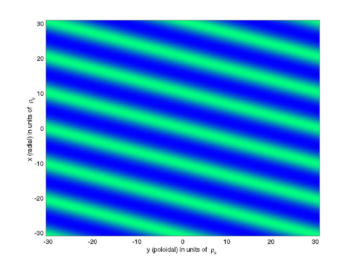
Figure 2: The same as Figure 1, in contour plot.

It is interesting to examine the structure of the flow field induced by the potential as a function of the position along the minor radius in tokamak. We first perform a numerical simulation using a one dimensional transport code [25]. Details are given in Appendix B. The physical data from simulation consists of

$$T_{e}\left(r\right),T_{i}\left(r\right),n\left(r\right),\rho_{s}\left(r\right),c_{s}\left(r\right),L_{n}\left(r\right),L_{T_{e}}\left(r\right),v_{\ast}\left(r\right)$$

which are transfered to a code that calculates the parameters $\alpha\left(r\right)$ , $\beta\left(r\right)$, $a\left(r\right)$, $b\left(r\right)$, $g_{2}\left(r\right)$ and, takes a fixed value for $g_{3}$. Then the half-periods $\omega\left(r\right)$ and $\omega^{\prime}\left(r\right)$ are calculated. These parameters are represented in the figures below.

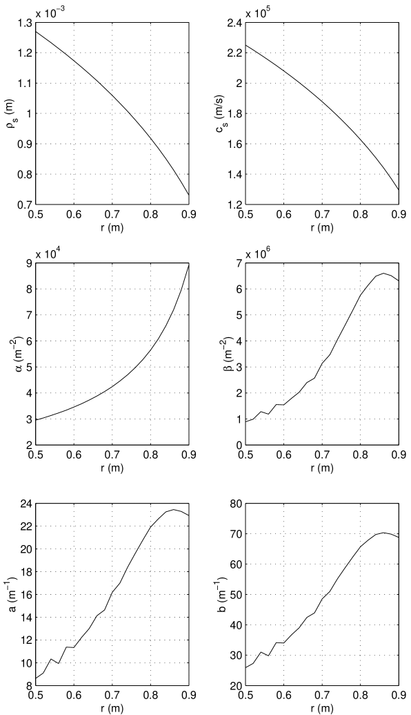
Figure 3: Physical parameters and the derived values $\alpha$ , $\beta$, $a$ and $b$ as function of $r$.

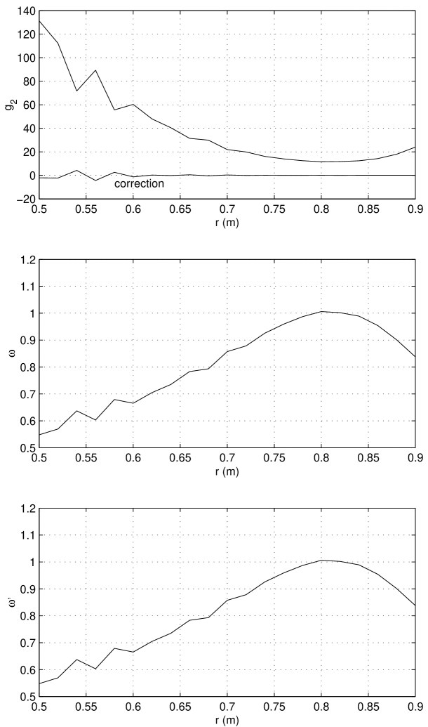
Figure 4: Plot of the parameters of the Weierstrass function. In the plot for $g_{2}$ the lower line represents the correction due to the space variation of the physical parameters.

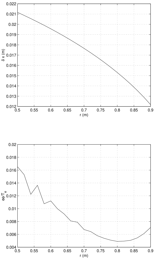
Figure 5: Width of the layer of flow and amplitude induced by the perturbation.

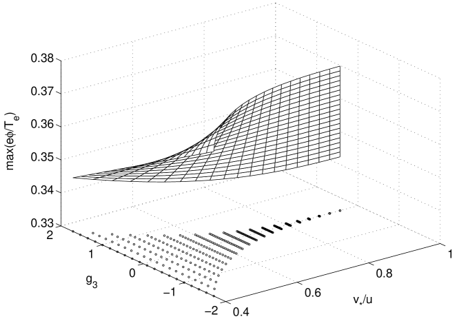
Figure 6: Variation of the amplitude $e\phi/T_{e}$ with $g_{3}$ and $v_{\ast}/u$.

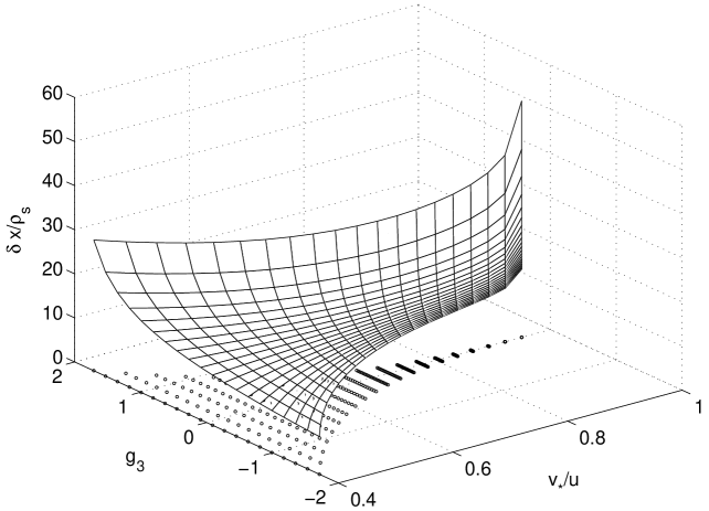
Figure 7: Variation of the width $\delta x$ of a layer with $g_{3}$ and $v_{\ast}/u$.

We have studied the effect of the variation of the second Weierstrass parameter, $g_{3}$. When it is taken equal to zero, we find that the width of the layer of poloidal flow, Eq.(55) is proportional to the local Larmor radius,

$$\delta x=3.924K\left(k^{\prime}\right)\left(1-v_{\ast}/u\right)^{-1/2}\rho_{s}$$

(with the constants of Eqs. (48) and (50)). The variations of the width of a layer $\delta x/\rho_{s}$ and of the maximum perturbation $e\phi/T_{e}$ with $g_{3}$ and $v_{\ast}/u$ are shown in Figs.6 and 7. On this graphs only the part where the discriminant of the Weierstrass function is positive $\Delta\equiv g_{2}^{3}-27g_{3}^{2}>0$ are shown, since there the roots $e_{1,2,3}$ are all real (these points are also indicated in projection on the plane). The characteristics of an initial physical field that can evolve toward this layered geometry of flow can be inferred from these graphs by eliminating the common variable $g_{3}$.

10 Conclusion

It has been known from the experiments on Rayleigh-Benard convection that at higher Reynolds number there is a second bifurcation (the first being from purely conducting to convective rolls phase) where the pattern of the fluid flow exhibits tilted structures. Close to the upper and to the lower boundaries there is a deformation of the rolls, the “wind” as has been designated, which significantly enhances the Reynolds stress and favorizes second instability and eventually global displacement of the fluid along the boundaries. This finding, supported independently by suggestive results from the numerical simulations of the ITG instability led to the idea that a tilting instability may favorise, by an increase of the Reynolds stress, the generation of zonal flow in plasma. The solutions we have found is a new factor that should be included in this physical description.

Certainly, the tilt of the radially elongated eddies specific to the ITG potential pattern can be favorable to the spontaneous generation of sheared poloidal flow. On the other hand, the solution we have found has a strong similarity to the tilted cells and zonal flows. It may be possible that after a certain degree of tilting is attained, the plasma evolves spontaneously to a solution of the type described above. This solution intrinsically consists of layers of sheared flow. What is more important is that this solution has all the usual attributes of an exactly integrable structure: it is more robust and may represent an attractor. It can be considered that relating the generation of the zonal flow to the process of evolution of a system to a robust attractor is a useful approach to be further examined.

In this work we have restricted to the nonlinear dynamics of the $2D$ structures. As a further extension of the nonlinear solution of electrostatic drift waves described by the Hasegawa-Mima equation, the electromagnetic $3D$ vortical motion has also been studied [26], [27]. In particular it has been shown that a $2D$ vortical motion in the $\left(r,\theta\right)$-plane propagates along the magnetic line of force. Nonlinear coupling of drift-shear Alfven waves may lead to a novel nonlinear solution. Recently this topic has been extended and the formulation has been updated in Ref. [28]. These are however out of the scope of the present work and will be a subject of future research.

Acknowledgements.

This work has been performed during the stay of two of the authors (M.O.V. and F.S.) at NIFS as visiting professors. They acknowledge the hospitality of Prof. M. Fujiwara and Prof. O. Motojima. This work is partially supported by the Grant-in-Aid for Scientific Research of MEXT Japan and by the collaboration programmes of the National Institute for Fusion Science and of the Research Institute for Applied Mechanics of Kyushu University.

Appendix A : Discussion on the weak space variation of the parameters

In order to obtain the exact solution we had to assume that the coefficients are constant. Later, we have considered a weak variation of the coefficients with the coordinate $x$, induced by the presence of the physical parameters. We can assume that this is a reasonable representation of the real situation only if we have an adiabatic variation of $g_{2}$ with the physical parameters.

The numerical study of the dependence of the elliptic function on the physical parameters shows that $g_{2}$ is indeed slowly varying and that the correction due to the second term in the expression of $g_{2}$ can be neglected.

One can see that the weaker restriction can be formulated as follows: $g_{2}$ is independent on $u=iay+ibx+\omega$, which means that $g_{2}$ is constant along the lines $ay+bx=const$ and can only have a slow parametric variation in the direction transversal to this family of lines. Taking into account the expression of $g_{2}$ and that $\alpha$ and $\beta$ has variation mainly along the radial direction, we can reformulate the restriction by requiring that $g_{2}$ has no variation along lines quasi-parallel to the poloidal dierction, and can only have a weak dependence perpendicular on these lines. This explains our choice of combination of $a$ and $b$ in the numerical study presented above.

We will make a scaling transformation to reduce the Weierstrass function to constant coefficient $g_{2}$. For this we recall the formula for homogeneity of the Weierstrass function

$$\wp\left(u;g_{2},g_{3}\right)=\mu^{2}\wp\left(\mu u;\frac{g_{2}}{\mu^{4}},\frac{g_{3}}{\mu^{6}}\right)$$ (A.1)

We take

$$g_{3}=0$$

$$\mu = g_{2}^{1/4}$$

$$= \left[\frac{3\alpha^{2}}{s^{2}\beta^{2}}-\frac{6}{s^{2}\beta}\Delta\left(\frac{\alpha}{\beta}\right)\right]^{1/4}$$

and the formula becomes

$$\wp\left(u;g_{2},g_{3}\right)=g_{2}^{1/2}\wp\left(g_{2}^{1/4}u;1,0\right)$$ (A.2)

or

$$\phi\left(x,y\right)=\frac{\alpha}{2\beta}+g_{2}^{1/2}s\wp\left(g_{2}^{1/4}\left(iay+ibx+\omega\right);1,0\right)$$ (A.3)

This formula may serve for a numerical investigation of the space variation and the estimation of the error in using the solution based on constant coefficients.

We ask the stronger condition, that $g_{2}$ is simply a constant

$$g_{2}=\frac{3\alpha^{2}}{s^{2}\beta^{2}}-\frac{6}{s^{2}\beta}\Delta\left(\frac{\alpha}{\beta}\right)=\text{const}$$

This is essentially a differential equation which strongly constrain the space dependence of the physical parameters. Taking for example const$=p$, and remembering that the physical variation is on $x$, we have

$$\frac{d^{2}}{dx^{2}}\left(\frac{\alpha}{\beta}\right)=\frac{\alpha^{2}}{2\beta}-\frac{\beta s^{2}p}{6}$$

Now we assume that the radial third derivative of the density is small and take then $\beta$ constant. The equation for $\alpha$ is

$$\alpha^{\prime\prime}=6\alpha^{2}-2\beta^{2}s^{2}p$$ (A.4)

after a dividing the variable $x$ with $\sqrt{12}$. This is again the Weierstrass equation and the solution is $\wp\left(x\right)$ where $x$ is measured from the surface where the periods are calculated. Looking for non-periodic solutions we find

$$\alpha\left(x\right)=1-\frac{v_{\ast}}{u}=\left(\frac{\beta^{2}s^{2}p}{3}\right)^{1/2}-\frac{3\left(\beta^{2}s^{2}p/3\right)^{1/2}}{\cosh^{2}\left[\sqrt{3}\left(\beta^{2}s^{2}p/3\right)^{1/4}\right]}$$ (A.5)

We see that the behaviour of the right hand side in Eq.(A.5) is approximately linear in the variable $\left(\beta^{2}s^{2}p/3\right)^{1/2}$. Then we can expect a condition of the form

$$\frac{v_{\ast}}{u}\approx\beta s\left(\frac{g_{2}}{3}\right)^{1/2}$$

or

$$\frac{\rho_{s}}{L_{n}}\approx\frac{c_{s}}{2u}\frac{d}{dx}\left(\frac{1}{L_{n}}\right)s\left(\frac{g_{2}}{3}\right)^{1/2}$$

Here all distances, $x$ and $L_{n}$ have been normalized at a typical Larmor radius, $\rho_{s0}$. This can be reduced to a condition on the density variation with the minor radius

$$\frac{d}{dr}\left(\ln\frac{1}{L_{n}}\right)\approx\left[s\left(\frac{g_{2}}{3}\right)^{1/2}\frac{\Omega_{i}}{2u}\right]^{-1}\sim 0.05$$

The conclusion is that the density gradient length has a variation of the type

$$L_{n}\sim\exp\left(-0.05\frac{x}{\rho_{s0}}\right)$$

on an interval $0<x<100\rho_{s0}$ in the region where this solution exists. The fast variation of the density is favorable to the validity of this solution.

Appendix B : Numerical simulation for tokamak plasma parameter’s profiles

The code [25] solves the balance equations for energy, density and fields. The variables are: the electron and ion temperatures $T_{e}$, $T_{i}$; the current density $j$, the poloidal magnetic field $B_{\theta}$, the toroidal electric field $E_{\varphi}$, the electron density $n_{e}$, the radial pinch particle velocity $V_{r}$. The following equations are discretized on a one-dimensional space mesh (on the small radius) and evloved in time by a semi-implicit scheme.

$$\frac{3}{2}\frac{\partial}{\partial t}\left(n_{e}T_{e}\right) = -\frac{1}{r}\frac{\partial}{\partial r}\left(r\left(-n_{e}\chi_{e}\frac{\partial T_{e}}{\partial r}+n_{e}VT_{e}\right)\right)+Ej$$

$$-3\frac{m_{e}}{m_{i}}n_{e}\frac{T_{e}-T_{i}}{\tau_{ei}}-P_{rad}-P_{ion}+P_{add}^{e}$$

$$\frac{3}{2}\frac{\partial}{\partial t}\left(n_{i}T_{i}\right) = -\frac{1}{r}\frac{\partial}{\partial r}\left(r\left(-n_{i}\chi_{i}\frac{\partial T_{i}}{\partial r}+n_{i}VT_{i}\right)\right)$$

$$+3\frac{m_{e}}{m_{i}}n_{e}\frac{T_{e}-T_{i}}{\tau_{ei}}-P_{cx}+P_{add}^{i}$$

$$j=\frac{1}{\mu_{0}}\frac{1}{r}\frac{\partial}{\partial r}\left(rB_{\theta}\right)$$

$$\frac{\partial B_{\theta}}{\partial t}=\frac{\partial E}{\partial r}$$

$$E=\eta j$$

$$\frac{\partial n_{e}}{\partial t}=\frac{1}{r}\frac{\partial}{\partial r}\left(rD\frac{\partial n_{e}}{\partial r}\right)+S_{ion}$$

$$V=\frac{1}{n_{e}}\left(D\frac{\partial n_{e}}{\partial r}+V_{pinch}\right)$$

Neutral atoms as well as impurities (Carbon, Oxygen, Iron, Wolfram, Molibden) are considered. The transport coefficients are those of the Merejkhin-Mukhovatov model and the specific parameters of the tokamak correspond to the Tore-Supra device. The run is extended over 20 seconds and the stationarity is reached within few seconds. Then we extract radial dependent plasma parameter from a time slice at about 13.5 seconds.

References

- [1] W. Horton and A. Hasegawa, Chaos 4 (1994) 227.
- [2] M. J. Ablowitz and H. Segur, Solitons and Inverse Scattering Transform, SIAM, 1981.
- [3] H. Tasso, Phys. Lett. A24 (1967) 618.
- [4] V. I. Petviashvili, Fiz. Plazmy 3 (1977) 270 [Sov. J. Plasma Phys. 3 (1977) 150].
- [5] V. P. Lakhin, A. B. Mikhailovskii and O. G. Onishcenko, Phys. Lett. A119 (1987) 348.
- [6] E. W. Laedke and K. H. Spatschek, Phys. Fluids 31 (1988) 1492.
- [7] K. H. Spatschek, E. W. Laedke, Chr. Marquardt, S. Musher and H. Wenk, Phys. Rev. Lett. 64 (1990) 3027.
- [8] G. R. Flierl, Dyn. Atmos. Oceans 3 (1979) 15.
- [9] B. B. Kadomtsev and V. I. Petviashvili, Sov. Phys. Doklady 6 (1970) 539.
- [10] V. I. Petviashvili, O. A. Pokhotelov, Fiz. Plazmy 12 (1986) 651 [Sov. J. Plasma Phys. 12 (1986) 657].
- [11] J. P. Boyd and B. Tan, Chaos, Solitons and Fractals 9 (1998) 2007.
- [12] B. Tan and J. P. Boyd, Wave Motion 26 (1997) 239.
- [13] V. E. Zakharov and E. A. Kuznetsov, Sov. Phys. JETP 39 (1974) 285.
- [14] J. Todoroki and H. Sanuki, Phys. Letters 48A (1974) 277.
- [15] H. Sanuki and G. Schmidt, J. Phys. Soc. Jpn. 42 (1977) 260.
- [16] H. Iwasaki, S. Toh and T. Kawahara, Physica D 43 (1990) 293.
- [17] D. H. Peregrine, J. Fluid Mechanics 27 (1967) 815.
- [18] P. F. Byrd and M. D. Friedman, Handbook of Elliptic Integrals for Engineers and Scientists, Springer-Verlag, New-York, 1971.
- [19] M. Mulase, in Perspectives in Mathematical Physics, Eds. R. Penner and T. S. Yau, (1994) 151.
- [20] D. V. Choodnovsky and G. V. Choodnovsky, Il Nuovo Cimento 40 B (1977) 339.
- [21] W. R. Thickstun, Journal of Mathematical Analysis and Applications, 55 (1976) 335.
- [22] B. Deconinck and H. Segur, Mathematical Physics, Analysis and Geometry 3 (2000) 49.
- [23] M. Makino, T. Kamimura and T. Taniuti, J. Phys. Soc. Jpn. 50 (1981) 980.
- [24] X. N. Su, W. Horton and P. J. Morrison, Phys. Fluids B3 (1991) 921.
- [25] F.Spineanu, M.Vlad, J.-D. Reuss, J.H. Misguich, Plasma Physics and Controlled Fusion 41 (1999) 485.
- [26] H. Sanuki and J. Weiland, J. Plasma Physics 23 (1988) 516.
- [27] J. Weiland, H. Sanuki and C. S. Liu, Phys. Fluids 24 (1981) 93.
- [28] S. Mahajan and J. Weiland, Plasma Physics and Controlled Fusion 42 (2000) 987.