Modern Michelson-Morley experiment using cryogenic optical resonators

Abstract

We report on a new test of Lorentz invariance performed by comparing the resonance frequencies of two orthogonal cryogenic optical resonators subject to Earth’s rotation over $\sim 1$ year. For a possible anisotropy of the speed of light $c$, we obtain $\Delta_{\theta}c/c_{0}=(2.6\pm 1.7)\cdot 10^{-15}$. Within the Robertson-Mansouri-Sexl test theory, this implies an isotropy violation parameter $\beta-\delta-\frac{1}{2}=(-2.2\pm 1.5)\cdot 10^{-9}$, about three times lower than the best previous result. Within the general extension of the standard model of particle physics, we extract limits on 7 parameters at accuracies down to $10^{-15}$, improving the best previous result by about two orders of magnitude.

Special relativity (SR) underlies all accepted theories of nature at the fundamental level. Therefore, it has been and must be tested with ever increasing precision to provide a firm basis for its future application. Such tests are also motivated by the efforts to unify gravity with the other forces of nature, one of the outstanding open challenges in modern science. In fact, many currently discussed models of quantum gravity do violate the principles of SR. In string theory, for example, violation of Lorentz invariance might be caused by spontaneous symmetry breaking KosteleckySSB ; in loop gravity, effective low–energy equations (e.g., modified Maxwell equations gambini ) that violate Lorentz invariance have been derived. Since the natural energy scale for quantum gravity is the Planck scale, $E_{p}\sim 10^{19}$ GeV, a direct experimental investigation of quantum gravity effects is not feasible. It is, however, possible to search for residual effects at an attainable energy scale in experiments of outstanding precision. High-precision bounds on Lorentz violation might give valuable hints for or against particular models of quantum gravity.

A sensitive probe for Lorentz violation (in electrodynamics) is the Michelson-Morley (MM) experiment MM , that even predated the formulation of SR. It tests the isotropy of the speed of light, one of SR’s foundations. In the classic setup, one compares the speed of light $c$ in two orthogonal interferometer arms by observing the interference fringes. If $c$ depends on the direction of propagation, the fringes move if the setup is rotated (using, e.g., Earth’s rotation or a turntable). In 1979, Brillet and Hall BrilletHall introduced the modern technique of measuring a laser frequency stabilized to a resonance of an optical reference cavity. The frequency of such a resonance is given by $\nu_{\rm cav}=mc/(2L)$, where $L$ denotes the cavity length and $m=1,2,\ldots$ the mode number. Thus, a violation of the isotropy of $c$ can be detected by rotating the cavity and looking for a resulting variation of $\nu_{\rm cav}$ by comparing the frequency of the cavity–stabilized laser against a suitable reference. In our experiment (Fig. 1), we compare the frequencies $\nu_{x}$ and $\nu_{y}$ of two similar cavities oriented in orthogonal directions, in analogy with the classical interferometer tests. Compared to the single–cavity setup, this arrangement doubles the hypothetical signal amplitude and provides some common–mode rejection of systematic effects.

Our results are obtained making use of the high dimensional stability of cryogenic optical resonators (COREs). Constructed from crystalline sapphire, COREs show a low thermal expansion coefficient ($10^{-10}/$K at 4.2 K) and a remarkable absence of creep (i.e., intrinsic length changes due to material relaxation); upper limits for the CORE frequency drift are $<2$ kHz/6 months and $<0.1$ Hz/h COREs , which makes COREs particularly well suited for high-precision measurements such as relativity tests Braxmaier ; MuellerASTROD . For the MM experiment, it allows us to rely solely on Earth’s rotation. This avoids the systematic effects associated with active rotation, which previous experiments had to use to overcome the creep of room temperature resonators made from glass ceramics, e.g. ULE (ultra–low–expansion), on the time–scale of a day.

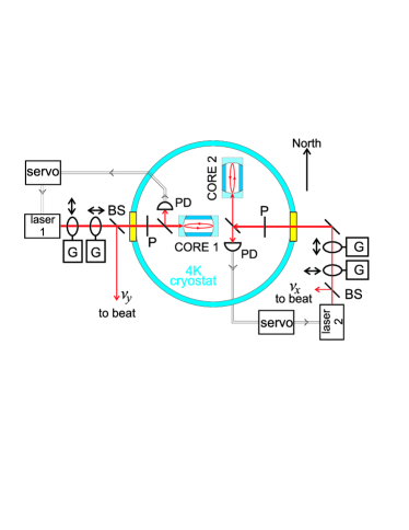
Figure 1: Setup. Inside a 4 K cryostat, two COREs are located in a copper block to provide common-mode rejection of thermal effects. LN2 is refilled automatically every $\sim 3$ h, LHe manually every $\sim 2$ days. Laser beams are coupled to the COREs via windows, with polarizers P and lock detectors PD inside the cryostat. For active beam positioning, beams pass through galvanomter (G) mounted glass plates. The horizontal and vertical displacements are adjusted to maximize coupling into the cavities, as measured using the $2f_{m}$ signal from the detector in reflection. Not shown is the setup for measuring the frequency difference $\nu_{x}-\nu_{y}$ of the lasers, in which the beams are overlapped on a high–speed photodetector and the beat frequency is measured against a quartz oscillator stabilized to the GPS.

A suitable theoretical framework for analyzing tests of Lorentz invariance is the general Standard Model Extension (SME) Kostelecky ; Kostelecky2002 . A Lagrangian formulation of the standard model is extended by adding all possible observer Lorentz scalars that can be formed from known particles and Lorentz tensors. In the Maxwell sector, the Lagrangian is $\mathcal{L}=\frac{1}{4}F_{\mu\nu}F^{\mu\nu}+\frac{1}{4}(k_{F})_{\kappa\lambda\mu\nu}F^{\kappa\lambda}F^{\mu\nu}$ comment2 . The tensor $(k_{F})_{\kappa\lambda\mu\nu}$ (the greek indices run from $0\ldots 3$) has 19 independent components; they vanish, if SR is valid. 10 of its components, that can be arranged into traceless symmetric $3\times 3$ matrices $(\tilde{\kappa}_{e+})^{AB}$ and $(\tilde{\kappa}_{o-})^{AB}$, describe polarization–dependent effects. They are restricted to $<2\cdot 10^{-32}$ by polarization measurements on light from astronomical sources Kostelecky2002 and are assumed to be zero in the following. The remaining 9 components describe boost invariance and isotropy of $c$ and can be arranged into traceless $3\times 3$ matrices $(\tilde{\kappa}_{e-})^{AB}$ (symmetric) and $(\tilde{\kappa}_{o+})^{AB}$ (antisymmetric) plus one additional parameter. They lead to a shift $\delta\nu$ of the resonance frequency of a cavity Kostelecky2002 with a characteristic time signature and can thus be measured in cavity experiments.

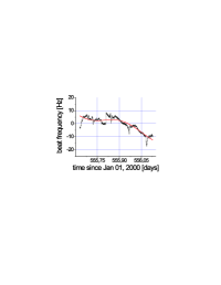
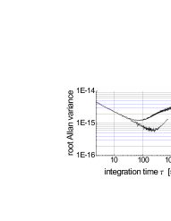
Figure 2: Left: Typical data set fitted with a 12 h sinewave amplitude, a linear drift, and a constant offset. Peaks occur every few hours due to automatic LN2 refills. Right: Root Allan variance calculated from this data (upper curve), and from a quiet part between two LN2–refills ($118$ minutes starting at 555.87 days; lower curve).

For our experiment (Fig. 1), we use two $L=3$ cm long COREs that feature linewidths of 100 kHz and 50 kHz, respectively, (Finesses $\sim 10^{5}$), located inside a liquid helium (LHe) cryostat with a liquid nitrogen (LN2) shield. Refills and the evaporation of coolants cause mechanical deformations of the cryostat, which change the resonator position. An automatic beam positioning system actively compensates for these movements (Fig. 1). The frequencies $\nu_{\rm las}$ of two diode-pumped Nd:YAG lasers at 1064 nm are stabilized (“locked”) to resonances of the COREs using the Pound-Drever-Hall method. The Nd:YAG laser crystal strain (generated by a piezo attached to the crystal) and temperature were used for tuning the frequency. The phase modulation at frequencies $f_{m}$ around 500 kHz is also generated by crystal strain modulation using mechanical resonances of the piezo. The light reflected from the COREs is detected inside the cryostat (Fig. 1) on Epitaxx 2000 InGaAs detectors. Down–conversion to DC at $3f_{m}$ rather than $1f_{m}$ reduces the influence of residual amplitude modulation and gives a higher signal-to-noise (S/N) ratio for the same circulating laser power inside the cavity. For the detector signal, amplifiers consisting of 8 paralleled BF1009 dual-gate MOSFETs provide low current noise in spite of the high detector capacitance (500 pF). At $\sim 80$ nW laser power impinging on the COREs, we achieve an error signal S/N ratio of $\sim 1.5\cdot 10^{4}\cdot\sqrt{\tau/\mbox{s}}$. Between $80\ldots 200$ nW have been used, minimizing the change of $\nu_{\rm cav}$ due to laser heating of the COREs ($\sim 10$ Hz/$\mu$W). The error signal is generated using mini-circuits ZHL-32 high-level amplifiers and SAY-1 23 dBm double-balanced-mixers operating at $\sim 0$ dBm RF amplitude and thus well below saturation. This provides highly linear operation and proved very important for a low sensitivity to systematic disturbances. On a time scale of minutes, we reach a minimum relative frequency instability of the lasers locked to the COREs of $7\cdot 10^{-16}$, referred to a single CORE (Fig. 2). Such a level is reached by the best ULE-cavity stabilized lasers bergquist only if a large linear drift $\sim 2$ Hz/s is subtracted.

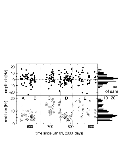
Figure 3: Fit results (upper part; dots) and fit residuals $\sqrt{\bar{\chi}^{2}}$ (lower part; crosses) for the amplitude of the cosine component of an assumed isotropy violation signal at $2\omega_{\oplus}$. Strongly perturbed data sets are omitted when $\sqrt{\bar{\chi}^{2}}>20$ Hz (25 subsets). In 8 of these cases, a good fit was achieved after discarding the first 1-3 hours (which likely contain residual perturbations from a preceding LHe refill); these were then re–introduced to the analysis. The histograms (bin size =1 Hz) on the right hand side give the distribution of the fit results and residuals.

A number of systematic disturbances (e.g. residual amplitude modulation, parasitic etalons, or mixer offset voltages) that cause lock–point shifts are compensated for using a new technique: By an additional phase modulation of the laser beams, a part of the laser power is shifted into side–bands, thus reducing the amplitude of the useful part of the error signal. If the parasitic effects do not have sufficient frequency selectivity to discriminate these sidebands against the carrier, modulating the amplitude of the sidebands makes the lock–point shifts time–dependent, so they can be identified and compensated for offsetkomp . This proved instrumental in achieving the reliable and repeatable laser system performance required for accumulating enough data.

Except for a 10 day break around New Year 2002, the COREs were operated continuously at 4.2 K over more than one year. Usable data (discounting data sets shorter than 12 hours and data taken during adjustment or LHe refills) starts June 19, 2001 and was acquired over 390 days until July 13, 2002. A total of 146 data sets of 12 h to 109 h in length, totaling 3461 h, are available (Fig. 2 and Fig. 3). 49 almost equally distributed data sets are longer then 24 h. For extracting results, simultaneous least–squares fits with a constant offset, a linear drift, and the amplitude of a sinusoidal signal at fixed frequency and phase as suggested by the test theory are performed. Before fitting, the data sets are divided into subsets of $12$ h (or 24 h for the 24 h signals). This drops a fraction of the data, but makes the resulting sinewave amplitudes independent of offsets in the data. We obtain 199 fits of 12 h data subsets (Fig. 3).

The individual fit results (Fig. 3) are combined for the final result by coherent (vector) averaging. In the SME, the hypothetical Lorentz violation signal $(\nu_{x}-\nu_{y})/\bar{\nu}=\sum_{i}A^{S}_{i}\sin\omega_{i}T_{\oplus}+A^{C}_{i}\cos\omega_{i}T_{\oplus}$, where $\bar{\nu}=(\nu_{x}+\nu_{y})/2$, has Fourier components at 6 frequencies $\omega_{i}$. As defined in Kostelecky2002 , $T_{\oplus}=0$ on March 20, 2001, 11:31 UT. The signal components as given in Tab. 1 are derived calculation from Eq. (39) in Kostelecky2002 (the cavity length $L$ is not substantially affected by the hypothetical Lorentz violation TTSME ). Because our data extends over more than one year, in the vector average we can resolve the 6 signal frequencies independence and extract elements of the traceless symmetric matrix

$$\tilde{\kappa}_{e-}=\left(\begin{array}[]{ccc}a&1.7\pm 2.6&-6.3\pm 12.4\\ 1.7\pm 2.6&b&3.6\pm 9.0\\ -6.3\pm 12.4&3.6\pm 9.0&-(a+b)\end{array}\right)\cdot 10^{-15}$$

with $a-b=8.9\pm 4.9$ (in the sun–centered celestial equatorial reference frame of Kostelecky2002 ). Likewise,

$$\tilde{\kappa}_{o+}=\left(\begin{array}[]{ccc}0&14\pm 14&-1.2\pm 2.6\\ -14\pm 14&0&0.1\pm 2.7\\ 1.2\pm 2.6&-0.1\pm 2.7&0\end{array}\right)\cdot 10^{-11}$$

for the antisymmetric matrix. One sigma errors are quoted. The limits on $\tilde{\kappa}_{o+}$ are weaker because its elements enter the experiment suppressed by $\beta_{\oplus}\sim 10^{-4}$, Earth’s orbital velocity. All elements of $\tilde{\kappa}_{o+}$ and all but one element of $\tilde{\kappa}_{e-}$ are obtained. Compared to Lipa , we improve the accuracy by about two orders of magnitude. Moreover, while Lipa give limits on linear combinations of the elements of $\tilde{\kappa}_{o+}$, the present experiment allows individual determination, because of the $>1$ year span of our data.

Table 1: Signal amplitudes $A^{S}_{i},A^{C}_{i}$ from the SME, based on Kostelecky2002 , and fit results. $\omega_{\oplus}\approx 2\pi/(23$h$56$min$)$ and $\Omega_{\oplus}=2\pi/1$ year denote the angular frequencies of Earth’s sidereal rotation and orbit; $\chi\approx 42.3^{\circ}$ is the colatitude of Konstanz, $\eta\approx 23.4^{\circ}$ the angle between the ecliptic and Earth’s equatorial plane. The signal includes contributions of order 1, or suppressed by either the Earth’s orbital velocity $\beta_{\oplus}\sim 10^{-4}$ or by the velocity of the laboratory due to Earth’s rotation $\beta_{L}\sim 10^{-6}$. For each $\omega_{i}$, we include only the largest term, in effect dropping all terms proportional to $\beta_{L}$. A fit result that has been used to extract a parameter of the SME is set in bold face. The unused fit results lead to additional (but weaker) limits on the elements of $\tilde{\kappa}_{o+}$.

$\omega_{i}$	$A^{S}_{i}$	Fit (Hz)	$A^{C}_{i}$	Fit (Hz)
$\omega_{\oplus}-\Omega_{\oplus}$	$\frac{\beta_{\oplus}}{2}\sin\chi\cos\chi[(\cos\eta+1)(\tilde{\kappa}_{o+})^{XY}-\cos\eta(\tilde{\kappa}_{o+})^{XZ}]$	${\bf 1.82\pm 1.91}$	$\frac{\beta_{\oplus}}{2}\sin\chi\cos\chi\sin\eta(\tilde{\kappa}_{o+})^{YZ}$	$0.67\pm 1.58$
$\omega_{\oplus}$	$-\sin\chi\cos\chi(\tilde{\kappa}_{e-})^{YZ}$	${\bf-0.51\pm 1.26}$	$-\sin\chi\cos\chi(\tilde{\kappa}_{e-})^{XZ}$	${\bf 0.89\pm 1.74}$
$\omega_{\oplus}+\Omega_{\oplus}$	$\frac{\beta_{\oplus}}{2}\sin\chi\cos\chi[(\cos\eta-1)(\tilde{\kappa}_{o+})^{XY}-\sin\eta(\tilde{\kappa}_{o+})^{XZ}]$	$-0.43\pm 1.68$	$\frac{\beta_{\oplus}}{2}\sin\chi\cos\chi\sin\eta(\tilde{\kappa}_{o+})^{YZ}$	$1.83\pm 1.83$
$2\omega_{\oplus}-\Omega_{\oplus}$	$-\frac{\beta_{\oplus}}{4}(1+\cos^{2}\chi)(\cos\eta+1)(\tilde{\kappa}_{o+})^{YZ}$	${\bf-0.01\pm 0.57}$	$-\frac{\beta_{\oplus}}{4}(1+\cos^{2}\chi)(1+\cos\eta)(\tilde{\kappa}_{o+})^{XZ}$	${\bf 0.25\pm 0.55}$
$2\omega_{\oplus}$	$\frac{1}{2}(1+\cos^{2}\chi)(\tilde{\kappa}_{e-})^{XY}$	${\bf 0.37\pm 0.56}$	$\frac{1}{4}(1+\cos^{2}\chi)[(\tilde{\kappa}_{e-})^{XX}-(\tilde{\kappa}_{e-})^{YY}]$	${\bf 0.97\pm 0.53}$
$2\omega_{\oplus}+\Omega_{\oplus}$	$\frac{\beta_{\oplus}}{4}(1+\cos^{2}\chi)(1-\cos\eta)(\tilde{\kappa}_{o+})^{YZ}$	$0.50\pm 0.55$	$\frac{\beta_{\oplus}}{4}(1+\cos^{2}\chi)(1-\cos\eta)(\tilde{\kappa}_{o+})^{XZ}$	$0.75\pm 0.58$

For comparison to previous work (e.g., BrilletHall ; grieser ; Braxmaier ; Wolf ), we also analyze our experiment within the Robertson-Mansouri-Sexl test framework RobertsonMS . It assumes generalized Lorentz transformations that contain parameters $\alpha,\beta$, and $\delta$. In a preferred frame $\Sigma$ (usually the cosmic microwave background), the speed of light $c_{0}$=const. In a frame $S$ moving with the velocity $\vec{v}$ with respect to $\Sigma$, $c/c_{0}=1-(A+B\sin^{2}\theta)v^{2}/c_{0}^{2}$, where $\theta$ is the angle between the direction of $c$ and $\vec{v}$. Both $A=\alpha-\beta+1$ and $B=\beta-\delta-\frac{1}{2}$ vanish in SR. In this formalism, SR follows from (i) Kennedy-Thorndike (KT)-, (ii) MM-, and (iii) Doppler shift experiments. The latter determine the time dilation coefficient $\alpha$ ($=-\frac{1}{2}$ in SR) to $|\alpha+\frac{1}{2}|<8\cdot 10^{-7}$ grieser . KT experiments test velocity invariance of $c$, using the periodic modulation of $v$ provided by Earth’s orbit Braxmaier or rotation Wolf . Measuring the frequency of a cryogenic microwave cavity (that is proportional to $c$) against an H-maser, Wolf obtained $A=(-3.1\pm 6.9)\cdot 10^{-7}$.

While all three experiments are required for a complete verification of SR within this framework, the MM experiment currently offers the highest resolution. In case of a violation of isotropy, $B\neq 0$, for our experiment we obtain a periodic change of the beat frequency $\nu_{x}-\nu_{y}$ at $2\omega_{\oplus}$ RMSderivation . For such a signal, the experiment yields an amplitude $1.03\pm 0.53$ Hz, or $B=(-3.1\pm 1.6)\cdot 10^{-9}$. As the quality of the data is not uniform (Fig. 3), taking a weighted vector average is more appropriate here independence . We divide the data into the intervals A-E (Fig.3) with approximately uniform data quality within each. The averages over the intervals are then combined to the final result, weighted according to their standard error. This leads to a signal of $0.73\pm 0.48$ Hz, or

$$B=\beta-\delta-\frac{1}{2}=(-2.2\pm 1.5)\cdot 10^{-9}\,,$$

which we regard as the final result within the RMS framework. It has an inaccuracy about three times lower than the best previous result $B=(3.0\pm 4.9)\cdot 10^{-9}$BrilletHall ; BHanalysis .

In summary, we performed a modern Michelson-Morley experiment by comparing the frequencies of two crossed cryogenic optical resonators subject to Earth’s rotation over a period spanning more than one year. Within the Robertson-Mansouri-Sexl framework, our limit on the isotropy violation parameter is about three times lower than that from the classic experiment of Brillet and Hall BrilletHall . Moreover, we obtain limits on seven parameters from the comprehensive extension of the standard model Kostelecky ; Kostelecky2002 , down to $10^{-15}$, about two orders of magnitude lower than the only previous result Lipa .
While the high long–term stability of COREs allows one to use solely Earth’s rotation, active rotation could still improve the accuracy significantly. Due to the low drift of COREs compared to ULE cavities, the optimum rotation rate would be relatively slow, which is desirable for minimizing the systematics. At a rate of $\sim 0.2$/min ($\sim 5$/min was used in BrilletHall ), one could utilize the optimum $\sim 7\cdot 10^{-16}$ frequency stability (Fig. 2) of the COREs, more than $10$ times better than on the 12 h time scale used so far. Since $\sim 500$ measurements (2 per turn) could be accumulated per day, one should thus be able to reach the $10^{-17}$ level of accuracy. Further improvements include fiber coupling and COREs of higher finesse. Finally, space based missions with resonators are currently studied (OPTIS OPTIS and SUMO SUMO ).

We thank Claus Lämmerzahl for many valuable discussions and Jürgen Mlynek for making this project possible. This work has been supported by the Deutsche Forschungsgemeinschaft and the Optik-Zentrum Konstanz.

References

- (1) V.A. Kostelecký and S. Samuel, Phys. Rev. D 39, 683 (1989).
- (2) R. Gambini and J. Pullin, Phys. Rev. D 59, 124021 (1999).
- (3) A.A. Michelson, Am. J. Sci. 22, 120 (1881); A.A. Michelson and E.W. Morley, ibid. 34, 333 (1887); Phil. Mag. 24, 449 (1897).
- (4) A. Brillet and J.L. Hall, Phys. Rev. Lett. 42, 549 (1979).
- (5) S. Seel et al., Phys. Rev. Lett. 78, 4741 (1997); R. Storz et al., Opt. Lett. 23, 1031 (1998).
- (6) C. Braxmaier et al., Phys. Rev. Lett. 88, 010401 (2001).
- (7) H. Müller et al., Int. J. Mod. Phys. D 11, 1101 (2002).
- (8) D. Colladay and V.A. Kostelecký, Phys. Rev. D 55, 6760 (1997); 58, 116002 (1998); R. Bluhm et al., Phys. Rev. Lett. 88, 090801 (2002), and references therein.
- (9) V.A. Kostelecký and M. Mewes, Phys. Rev. D 66, 056005 (2002).
- (10) Additional parameters are strongly bounded by other experiments Kostelecky2002 and assumed to be zero here.
- (11) B.C. Young et al., Phys. Rev. Lett. 82, 3799 (1999).
- (12) H. Müller et al., to be published
- (13) For our cavity orientation (one cavity pointing north, the other west), the terms proportional to (that in part depend on the transverse relative permittivity inside the resonator) and , as defined in Kostelecky2002 , drop out. We substitute , as given in appendix E of Kostelecky2002 into Eq. (39) of that paper. The difference between the two time–scales and used in Kostelecky2002 , hours for our experiment, gives rise to additional terms proportional to that can be neglected.
- (14) H. Müller et al., Phys. Rev. D 67, 056006 (2003).
- (15) In the SME analysis, unweighted averages are taken, since weighted averages here would increase the interdependence of the fit results, typically and in all cases . We can neglect it for the present purpose.
- (16) J.A. Lipa et al., Phys. Rev. Lett. 90 060403 (2003).
- (17) P. Wolf et al., Phys. Rev. Lett. 90 060402 (2003).
- (18) R. Grieser et al., Appl. Phys. B 59, 127 (1994).
- (19) H.P. Robertson, Rev. Mod. Phys. 21, 378 (1949); R.M. Mansouri and R.U. Sexl, Gen. Rel. Gravit. 8, 497 (1977); 8, 515 (1977); 8, 809 (1977); see also C. Lämmerzahl et al., Int. J. Mod. Phys. D 11, 1109 (2002).
- (20) (plus negligible Fourier components), obtained by expressing the angles and between the cavity axes and in terms of , the declination of , and km/s lin96 . on March 8, 2001, 11:34 UT, when the west-pointing resonator is orthogonal to the projection of onto the equatorial plane.
- (21) The result is quoted here assuming km/s lin96 and taking into account a factor for the colatitude of the laboratory in Boulder.
- (22) C. Lämmerzahl et al., Class. Quant. Grav. 18, 2499 (2001).
- (23) S. Buchman et al., Adv. Space Res. 25, 1251 (2000).
- (24) C. H. Lineweaver et al., Astropys. J. 470, 38 (1996).