Heterodyne Near-Field Scattering

Abstract

We describe an optical technique based on the statistical analysis of the random intensity distribution due to the interference of the near-field scattered light with the strong transmitted beam. It is shown that, from the study of the two-dimensional power spectrum of the intensity, one derives the scattered intensity as a function of the scattering wave vector. Near-field conditions are specified and discussed. The substantial advantages over traditional scattering technique are pointed out, and is indicated that the technique could be of interest for wave lengths other than visible light.

Scattering techniques represent a powerful tool to probe the structure of matter. Syncrotron radiation, neutron and light scattering allow to investigate phenomena occurring across a wide range of lengthscales, spanning from the atomic one up to fractions of a millimeter. Scattering is used for the determination of the structure factor of liquids, macromolecules, gels, porous materials and complex fluids, by detecting the intensity $I_{S}\left(\Theta\right)$ of the scattered radiation in the far field as a function of the scattering angle $\Theta$. Each point in the far field is illuminated by radiation coming from different portions of the sample, and the superposition of the scattered fields with random phases gives rise to coherence areas (speckles) goodman . According to Van Cittert and Zernike theorem, the size and shape of the speckles in the far field is related to the intensity distribution of the probe beam. All the classical techniques rely on the measurement of the average scattered intensity, and no physical information can be gained from the statistical analysis of the far field speckles.

In this paper we will describe a scattering technique based on the statistical analysis of the random intensity modulation due to the interference of the strong transmitted beam and the near field scattered light. We will show that one can derive the scattered intensity distribution $I_{S}\left(\Theta\right)$ from the two dimensional power spectrum of the intensity fluctuations. The Heterodyne technique is a more powerful and simpler alternative to the Homodyne Near Field Scattering that we have recently presented carpineti2000 ; carpineti2001 . It offers many substantial advantages over the homodyne technique and the conventional small angle light scattering. There is no need of the rather awkward block of the transmitted beam as in the homodyne case, and this makes the layout very simple and with no necessity of any alignment. It allows rigorous (static) stray light subtraction without any blank measurement. Also, being a self referencing technique, it allows to determine absolute differential scattering cross sections. It also has a wide dynamic range, since the signal depends on the amplitude of the scattered fields and not on the scattered intensities. Finally, it gives much improved statistical accuracy. It is worth pointing out that in principle the technique can be used with other type of scattering, like syncrotron or FEL radiation, or whenever coherence properties are adequate to generate speckles.

The following discussion provides the rationale behind the heterodyne technique.

As in classical light scattering, we send a collimated laser beam with wave vector $\vec{k}_{0}$ through a sample, and our goal is to measure $I_{S}\left(Q\right)$, the intensity of the light scattered at wave vector $\vec{k}_{S}$ as a function of the transferred momentum $\vec{Q}=\vec{k}_{S}-\vec{k}_{0}$. In the technique presented here, this task is accomplished by measuring and analyzing the intensity of light in a plane near the cell, in the forward scattering direction (see Fig. 1),

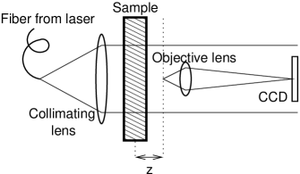
Figure 1: The optical layout of the instrument. The diverging laser beam from the fiber is collimated and sent through the sample. A microscope objective images onto a CCD detector a plane at a distance $z$ from the cell.

perpendicular to the direction of the incident beam, where the intense transmitted light acts as a reference beam interfering with the weak scattered beams. Then, in the sensor plane $\left[x,y\right]$, the intensity $I\left(x,y\right)$ is the sum of the strong transmitted beam intensity $I_{0}$ and of the small modulations $\delta I\left(x,y\right)$, due to the interference of the transmitted beam with the scattered beams (heterodyne term); terms arising from the interference between scattered beams can be neglected (homodyne terms). The intensity modulation $\delta I\left(x,y\right)$, in the plane $\left[x,y\right]$, can be decomposed in its Fourier components, with amplitude $\delta I\left(q_{x},q_{y}\right)$. A modulation with wave vector $\left[q_{x},q_{y}\right]$ is generated by the interference of the transmitted beam with a scattered three-dimensional plane wave with wave vector $\vec{k}_{S}=\left[q_{x},q_{y},k_{z}\right]$ or $\vec{k}_{S}=\left[-q_{x},-q_{y},k_{z}\right]$. Both the waves contribute to the heterodyne signal:

$$\delta I\left(q_{x},q_{y}\right)\propto\Re\left[\delta E\left(q_{x},q_{y},k_{z}\right)+\delta E\left(-q_{x},-q_{y},k_{z}\right)\right]$$ (1)

where $\delta E\left(q_{x},q_{y},k_{z}\right)$ and $\delta E\left(-q_{x},-q_{y},k_{z}\right)$ are the amplitudes of the two scattered waves, travelling at symmetric angles with respect to the direction of the probe beam. Because the scattering we are considering is elastic, the only possible value of $k_{z}$ can be determined by imposing the condition $\left|\left[q_{x},q_{y},k_{z}\right]\right|=k$, where $k=\left|\vec{k}\right|$. We can thus easily evaluate the modulus of the transferred wave vector $Q$, corresponding to the plane wave responsible for the modulation of the intensity on the plane, with wave vector $q$:

$$Q\left(q\right)=\sqrt{2}k\sqrt{1-\sqrt{1-\left(\frac{q}{k}\right)^{2}}},$$ (2)

which can be approximated by $Q\left(q\right)=q$, in the limit of small scattering angles. The scattered intensity $I_{S}\left(Q\right)$ is simply related to the power spectrum $S_{\delta I}\left(q\right)$ of the intensity modulations in the detector plane. By taking the mean square modulus of both sides of Eq. (1) we obtain:

$$S_{\delta I}\left(q\right)\propto I_{S}\left[Q\left(q\right)\right]+\left<\Re\delta E\left(q_{x},q_{y},k_{z}\right)\Re\delta E\left(-q_{x},-q_{y},k_{z}\right)\right>.$$ (3)

Neglecting the correlation term of the two fields, we have:

$$S_{\delta I}\left(q\right)\propto I_{S}\left[Q\left(q\right)\right].$$ (4)

In practice the measurement of the intensity modulations is implemented by using an array detector, which maps the intensity as a function of position $\delta I\left(x,y\right)$. The evaluation of $S_{\delta I}\left(q\right)$ can then be easily performed by a suitable processing.

The distance $z$ between the sample and the detector plane must meet two conditions, that we will discuss below.

Let us consider a sample whose diffraction halo is contained within an angle $\Theta^{*}$. The detector is then hit by light coming from a circular region of the sample with diameter $D^{*}\approx z\Theta^{*}$. Equation (4) holds for the ideal case of an infinite incoming wave with infinitely wide sample. In order for Eq. (4) to be valid for a finite size geometry, we must have that $D^{*}$ is much smaller than the main beam diameter $D$ that we assume of uniform intensity. The condition then is $z<D/\Theta^{*}$.

We now discuss the second condition on $z$. Eq. (4) holds if $\delta E\left(q_{x},q_{y},k_{z}\right)$ and $\delta E\left(-q_{x},-q_{y},k_{z}\right)$ are not correlated. A typical situation in which this does not happen is the case of the Raman-Nath scattering regime, where the sample can be approximated as a two dimensional phase grating, and the fields scattered at symmetric angles do bear a definite phase relation. Consequently the system shows the more complex behaviour described as the Talbot effect goodman . In particular, in spite of the fact that the grating scatters light at two symmetric angles, at periodic values of the sensor distance $z$, the interference with the transmitted beam does not give rise to any intensity modulation. This is the regime in which works the shadowgraph technique cannell1995 .

In order for the two fields not to be correlated, we must place the sensor not too close to the sample. Since the detector area $A$ is finite, the wave vectors $\left[q_{x},q_{y}\right]$ are discrete and correspond to the Fourier modes of $A$. Therefore, each mode corresponds to a discrete scattering range of directions we can resolve. The light hitting the area $A$ comes from different regions of the sample, one for each scattering direction. In order for the phase relations to vanish, the distance $z$ must be so large that the portion of the scattering volume feeding light scattered at $\left[q_{x},q_{y},k_{z}\right]$ to the detector does not overlap with the portion of the scattering volume feeding light at $\left[-q_{x},-q_{y},k_{z}\right]$. The resulting condition is $z>L^{2}/\lambda$, where $L$ is the transverse dimension of the sensor, and $\lambda$ is the wave length of the light used.

For ordinary samples, the mean distance $\delta$ between the scatterers is such that $\delta\ll L$. In this case, it can be easily shown that the condition above guarantees that the scattered field is a gaussian random process.

To evaluate the performances of the technique we have performed measurements on water suspensions of colloidal latex particles; the wave vector range covered roughly two decades of $q$ wave vectors.

The optical layout of the instrument is shown in Fig. 1. The collimated and spatially filtered beam coming from a 10 mW He-Ne LASER impinges onto the sample contained in a parallel walls cuvette. The beam diameter corresponds to 21 mm at $1/e$. A 20X microscope objective images onto a CCD detector a plane placed 15 mm after the cell. The CCD is an array of $768\times 576$ square pixels each having a size of $8\mu\mathrm{m}$. The intensity distribution onto the CCD is a 20X magnified replica of the intensity of this pattern. The magnification has been selected so that the wave vector range we want to measure corresponds to lengths between the pixel dimension and the sensor dimension. These magnified speckle patterns $I\left(x,y\right)$ represent the raw data, from which the scattered intensity distribution $I_{S}\left(Q\right)$ can be derived according to the the following procedure. First, a sequence of about 100 images is grabbed and stored. The images are spaced in time so that the speckle fields in the images are statistically independent. This is achieved by grabbing images at a frequency smaller than the smallest characteristic frequency of the sample, in our case $DQ_{\min}^{2}$, where $D$ is the diffusion coefficient of the latex particles and $Q_{\min}$ is the smaller wave vector detected by the CCD ($Q\simeq$20cm^-1 for our setup). The time average $\tilde{I}\left(x,y\right)$ of the set of images is then subtracted from each image, and the result is normalized by the spatial average $I_{0}$ of $\tilde{I}\left(x,y\right)$:

$$i\left(x,y\right)=\frac{I\left(x,y\right)-\tilde{I}\left(x,y\right)}{I_{0}}$$ (5)

Basically $\tilde{I}\left(x,y\right)$ represents an optical background due to the non-uniform illumination of the sample. This background is subtracted so to obtain the spatially fluctuating part of the signal. The spectrum of the normalized signal is then calculated from the Fast Fourier Transform of the normalized intensity by using Parseval’s relation, $S(q_{x},q_{y})=|F[i(x,y)]|^{2}$. After the azimuthal average of the power spectrum, the scattered intensity is finally obtained from Eq. (4), where the wave vectors are rescaled according to Eq. (2).

Data obtained for the intensity scattered in the Mie regime by water suspension of latex colloidal particles are presented in Fig. 2.

Figure 2: Light scattering from a water suspension of $5.2\mu\mathrm{m}$ and $10\mu\mathrm{m}$ latex colloidal particles, measured by Small Angle Light Scattering (SALS) and Heterodyne Near Field Scattering.

The two data-set correspond to 5.2$\mu$m and 10$\mu$m diameter particles. The concentration was such that the fraction of power of the probe beam removed due to scattering was of the order of a few percent, so that the self-beating contribution of the scattered light is negligeable. Figure 2 also shows data obtained from the same samples by using a state-of-the-art small-angle light scattering machine carpineti1990 ; ferri1997 across two decades in wave vector. Data from the heterodyne technique closely mirror those obtained by means of small angle light scattering.

We believe that visible light Heterodyne Near Field Scattering is a promising technique, particularly well suited to replace the more traditional low angle light scattering. Typical applications will include colloids, aggregates, particulate matter, aerosols, phase transitions and complex fluids in general. Finally, we point out that X Ray sources like the FEL should have fairly good coherence properties TESLA . The required magnification to bring the X Ray speckle size to realistic dimensions and larger than the available pixel sizes could be obtained by the use of properly diverging beams (not discussed here) and long distances between the sample and the sensor.

We thank Marco Potenza for useful discussion.

References

- (1) J. W. Goodman, Statistical Optics, Wiley, New York, 1985.
- (2) M. Giglio, M. Carpineti, and A. Vailati, Phys. Rev. Lett. 85, 1416 (2000).
- (3) M. Giglio, M. Carpineti, A. Vailati, and D. Brogioli, Applied Optics 40, 4036 (2001).
- (4) M. Wu, G. Ahlers, and D. S. Cannell, Phys. Rev. Lett. 75, 1743 (1995).
- (5) M. Carpineti, F. Ferri, M. Giglio, E. Paganini, and U. Perini, Phys. Rev. A 42, 7347 (1990).
- (6) F. Ferri, Rev. Sci. Instrum. 68, 2265 (1997).
- (7) G. Materlik and T. Tschentscher, editors, TESLA: The Superconducting Electron-Positron Linear Collider with Integrated X-Ray Laser Laboratory, volume V: The X-Ray Free Electron Laser, DESY, Hamburg, 2001.