Dynamical system analysis and forecasting of deformation produced by an earthquake fault
Abstract
We present a method of constructing low-dimensional nonlinear models describing the main dynamical features of a discrete 2D cellular fault zone, with many degrees of freedom, embedded in a 3D elastic solid. A given fault system is characterized by a set of parameters that describe the dynamics, rheology, property disorder, and fault geometry. Depending on the location in the system parameter space we show that the coarse dynamics of the fault can be confined to an attractor whose dimension is significantly smaller than the space in which the dynamics takes place. Our strategy of system reduction is to search for a few coherent structures that dominate the dynamics and to capture the interaction between these coherent structures. The identification of the basic interacting structures is obtained by applying the Proper Orthogonal Decomposition (POD) to the surface deformations fields that accompany strike-slip faulting accumulated over equal time intervals. We use a feed-forward artificial neural network (ANN) architecture for the identification of the system dynamics projected onto the subspace (model space) spanned by the most energetic coherent structures. The ANN is trained using a standard back-propagation algorithm to predict (map) the values of the observed model state at a future time given the observed model state at the present time. This ANN provides an approximate, large scale, dynamical model for the fault. The map can be evaluated once to provide short term predictions or iterated to obtain prediction for the long term fault dynamics.
1 Introduction
A first principles approach to modeling and forecasting the dynamics of an earthquake fault is not feasible at present because the governing physical laws, geometric and structural fault properties, and controlling variables (fault stresses and slips) are not fully available. A practical alternative is to build “phenomenological” models that attempt to estimate the overall character of the system’s dynamics. These models quantify basic deterministic or stochastic relationships involving only a few irreducible degrees of freedom, which may be used for short-term prediction. We show that for earthquake forecasting this can be done using the spatio-temporal strain patterns embedded in the observable surface displacements. Such an approach is based on the observation that the large scale dynamics of the system often evolves on a manifold (or invariant measure for the case of strange attractors) with a dimension that is significantly smaller than that of the system’s phase space. In such cases, a few macroscopic observables can approximate very well the present state of the system and predictive models based on the dynamics of a reduced number of macroscopic observables can then be constructed.
In order to identify meaningful low-dimensional structures, we apply the Proper Orthogonal Decomposition (POD) - also known as the Principal Component Analysis (PCA) or Karhunen-Loève expansion - to an ensemble of surface deformation data generated by the system’s dynamics. The POD provides the most efficient way of capturing the dominant components of a dynamical process with only finitely many, and often surprisingly few, ”modes” [17]. Using synthetic calculations for a strike-slip fault system, we show that a reduced number of deformation modes can explain on the average the large scale dynamics of elastic surface deformations. The dynamics of these modes live on a low-dimensional ”reduced” attractor in the neighborhood of which the system spends most of its time. The state of the system in this reduced space - model state space - is represented by a set of modal coefficients that measures the projection of the ground surface deformation onto each dominant mode. Our goal is to extract the nonlinear modal dynamics in this model space by constructing a map of the observed model state at a future time given the observed model state at present time. We will present preliminary results in which an artificial neural network has been used with promising success to learn the dynamics of the reduced model from these modal time series. The reconstructed map has been iterated to obtain predictions for the long term model dynamics starting from its current model state. A rough test of the reliability of the model forecast to approximate the future of the fault system is also discussed.
Our method may be compared to the linear pattern dynamics introduced by Rundle and his coworkers [25]. Their technique is based upon a Karhunen-Loève expansion of the spatio-temporal seismicity data and is used to estimate a linear stochastic model for the evolution of a probability density function for seismic activity. In contrast to that method, which provides a local linear approximation in a probability space, we propose a global nonlinear approximation that describes the effective large-scale dynamics in a low-dimensional phase space.
2 Description of the Earthquake System
We distinguish between the assumed physical system and the model which is an approximate representation of the system. The assumed system is itself a simplified representation of fault systems in the earth, but will be considered a valid description of reality if its behavior is typical for the dynamics of an isolated fault. Our goal is to build data driven models, with useful predictive skills, which approximate the large scale dynamics of the system. If this is possible, we can conclude that the methods we propose can then be extrapolated to real isolated faults and, perhaps, even to complex fault systems.
Our assumed system corresponds to a discrete strike-slip fault of length km and width km embedded in a elastic continuum [3, 5]. The fault consists of a uniform grid of dynamical cells where slip is governed by static/kinetic friction processes, surrounded by regions with imposed constant slip rate of mm/year, representing the tectonic loading. We divide the 70 km 17.5 km computational grid into 128 32 square cells, with length and depth having equal dimensions of approximately 550 m, that corresponds to the dimension of small, effectively disconnected, slip patches in mature fault zones [5]. The brittle deformation at any fault position and time is governed by quasi-static, elastic dislocation theory and spatially varying “macroscopic” constitutive parameters that describe the static and kinetic friction processes. The stress at any fault position (cell) increases with time, (measured in years), due to the gradual tectonic loading and the time-dependent brittle deformation at other fault locations. It can be written as a boundary integral over the slip deficit ,
| (1) |
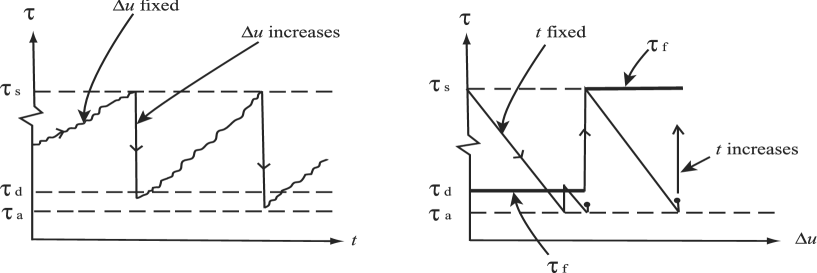
where is the elastic stress transfer function based on the solution of Chinnery [10], is the right lateral slip at fault cell ( measured in mm), and the summation is over the brittle area, 70 km 17.5 km, of the fault plane. The cell indexes and along the horizontal and vertical directions, respectively, define the spatial cell location. We assume that the static brittle strength is uniform along the fault and is set to a value of bars. If the stress reaches the static strength , a brittle failure occurs at this location and the cell slips an amount , till the local stress drops to a prescribed arrest stress level, . The stress transferred from the failed cell can lead to subsequent brittle failures (i.e., rupture propagation) if the stress anywhere increased to the failure threshold. These failures may, in turn, induce or reinduce more brittle slip events. After an initial slip event the strength drops to a dynamic level, , and reinitiation of brittle slip on an already failed cell occurs when there. The brittle slip associated with a stress drop can be described by
| (2) |
where is the self stiffness of a cell and the failure stress equals the static failure stress, , for a cell which has not slipped or is adjusted to its dynamic value, , every time a cell has failed. Figure 1 shows a schematic stress-time and stress-slip history for an individual cell. During an iteration loop, all failing cells are identified and their slips updated according to Eq. (2). At the end of each iteration the stress field is updated everywhere according to Eq. (1). The iterations end when there are no more brittle instabilities. This marks the end of an earthquake event whose strength is measured by its potency defined [7] as the integral of slip over the rupture area,
| (3) |
where and is the total slip at cell . During a seismic event the tectonic slip, , remains constant. At the end of each event the failure strength everywhere on the fault recovers back to . In order to initiate the next seismic event we advance in Eq. (1) the tectonic slip (or equivalently, advance the time ) till the fault cell closest to failure reaches its static failure strength. This triggers a new seismic event and starts again the failure iteration loops.
An important component of the fault rheology is the distribution of arrest and dynamic stresses along the fault. In the simulations used in this paper we chose random stresses,
| (4) |
where is the fault-averaged arrest stress, is a random number uniformly distributed in the range , and is the noise amplitude. The static strength, dynamic strength, and arrest stress are related to each other, at each point on the fault, as
| (5) |
where is a dynamic overshoot coefficient. Its inverse, , proportional to , is a measure of the dynamic weakening that characterizes static/kinetic friction models. The arrest and dynamic stress distributions do not evolve in time (quenched heterogeneities) and the fault dynamics is deterministic. We also assume no observational errors. We record the fault evolution after all transients have died out and the dynamics have reached a statistical steady-state (all moments of the stress and displacement fields become time independent). A thorough motivation of the fault system, based on a wealth of observations and numerical results, is provided in a series of papers by Ben-Zion and Rice [4, 3, 5], while a detailed description of the dynamics can be found in [2, 4, 6].
3 Qualitative dynamics of slips, stresses, and seismicity
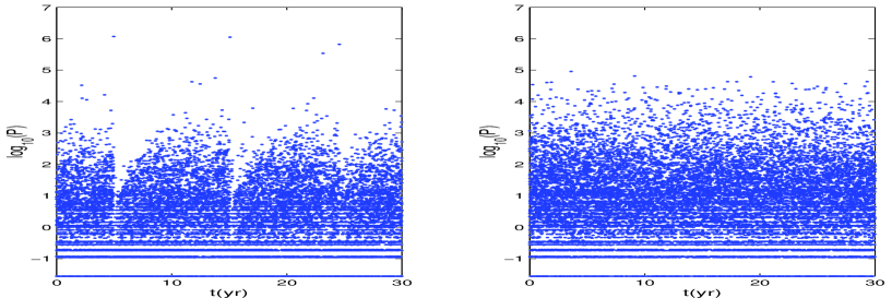
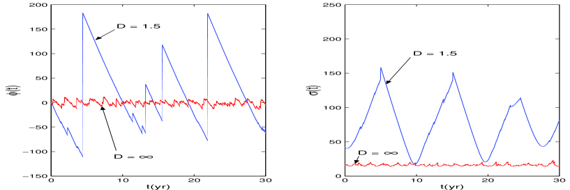
We start by analyzing the evolution of seismicity and the dynamics of the first and second order moments of the stress and slip fields. Here we only investigate the dynamics of two fault realizations that differ largely in the value of the dynamic overshoot coefficient. System with has a large dynamic weakening, while system with has no dynamic weakening. Both systems have random arrest stress distributions, as in (4), with bars and bars amplitude. A detailed investigation of the dynamics, covering the system space between these two limits, will be presented elsewhere [2]. In general, each system observable contains a different amount of information for understanding the underlying dynamics. As discussed below, for prediction purposes we are only interested in the dynamics at the large length and time scales. As the small scale dynamics overwhelmingly dominates the statistics, it is not obvious a priori which observable provides information about the large scale dynamics. In Fig. 2 we present the time evolution of the potency released over a 30 years time interval. The fault motion in system B () seems to be dominated by erratic, random appearing evolution. There are no detectable time patterns. When significant dynamic weakening is present, as in system A (), a clear signature of a quasi-regular evolution emerges. This can be identified in the presence of very large events (these are large scale events in which a large fraction of the fault slips), followed by intervals of seismic quiescence. There is a quasi-regular build up of correlations [6] which ultimately generates very large events, much larger in size than in system B. Although the evolution of seismicity is dominated by small events, there are significant evolution patterns reflecting the dynamics of the large scale events. These can be better seen in Fig. 3 which shows the evolution of the average slip deficit,
| (6) |
and slip deficit variance,
| (7) |
Due to the inhomogeneity of the slip deficit, the slip fluctuations are measured from a local time average, , defined as
| (8) |
where the length of the averaging time used is years. For the system we observe large seismic cycles and smooth long term behavior between two consecutive large events. At the scale of the plot in Fig. 3, the erratic and unpredictable small scale dynamics is unobservable. Magnifying the plot will reveal small scale jitters superposed over the smooth large scale motion. This suggests a clear separation of time scales between the slow, large scale motions and the fast, small scale motions. In contrast, the system has small oscillations and noisy behavior; note the large difference in the scale of the variance evolution for these two systems. For the system there are no large scale features and the dominant signature of small scale events renders the system higher dimensional. Additional illustrations of the dramatic change in the dynamics for cases with and without dynamic weakening are given in [6].
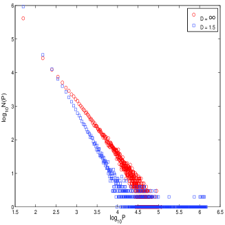
The emergence of a clear separation of length scales is also revealed in the frequency-size statistics shown in Fig.4. The system has a power-law distribution with an exponential cutoff, characteristic of systems close to a critical point. This confirms the analysis of Fisher et al. [11], who showed that the dynamic weakening is a tuning parameter and found that the system has an underlying critical point of second order phase transition at zero dynamic weakening () and full conservation of stress transfer during failure events. The frequency-size statistics for the system shows the existence of two separate earthquake populations. At small scales we observe a power-law distribution of event sizes. The other events cover a broad range of scales and their frequency is significantly higher than an extrapolation based on the power-law statistics of the small events. This behavior is reminiscent of the characteristic earthquake model [30, 7], which has a distinct probability density peak at the large size end of the frequency-size distribution. Moreover, a careful analysis [2] has shown that most stress dissipation is produced at the large size end of the potency spectrum and is due to the large scale motions. Averaged over small time intervals, the small events that dominate the frequency-size histogram do not produce any stress dissipation on average and only transfer stresses internally. This suggests a possible description of the dynamics in terms of large scale dissipative motions, that balance the stress increment due to an effective loading rate, which absorbs most of the small scale events into a renormalized plate velocity. This coarse-grained dynamics is inherently of lower dimension than the original dynamics. The question is whether the dimension collapse is significant to render data driven model reconstruction algorithms practical.
4 Effective dimension of the large scale motions
For the class of systems discussed in this paper the knowledge of the slip deficit, , where and , fully specifies the state of the fault; the number of microscopic degrees of freedom is and the state of the system is completely represented by a vector in a finite, but high-dimensional vector space , where . We conjecture that a finite dynamic weakening favors the creation of spatial and temporal correlations that collapse the asymptotic, long time dynamics of the fault onto an attractor of a smaller effective dimension ; . This is compatible with the recent analysis of Ben-Zion et al. [6]. The physics of the dimensional collapse consists in the clear separation of time and length scales. In such cases, we can in principle isolate the large scale dynamics which, evolving slowly, will drive the rapidly relaxing small scale dynamics. But, are real faults characterized by a large dynamic weakening? Full elastodynamic simulations of rupture propagation in a 3D elastic solid [20] indicate that , corresponding to large dynamic weakening. Moreover, we have shown elsewhere [2] that this separation of scales holds for a broad range of values and is, therefore, generic. Consequently, restricting our study to system A, we shall address for the rest of this paper the following issues (1) Whether we can build a predictive model for the large scale motions and (2) What effect the neglected small scale motions have on the predictability of the larger scales.
In order to model the large scale motions we have to find first if their dynamics is deterministic in character. In principle, the coarse grained dynamics of any deterministic system is stochastic. When a separation of scales exists, we can assume that only the statistical properties of the small scale motions influence the larger scales, through coefficients of turbulent viscosity, and that at any moment these statistical properties are determined by the larger scale motions [19]. A model describing only the large scale dynamics is assumed to be effectively deterministic. However, we have to be careful, because, as pointed out by Lorenz [19], there remains uncertainties in these statistics, and their progression to the very large scales will ultimately produce large scale errors and limit the forecasting skill of our model. We will therefore assume, as a working hypothesis, that a model describing only the larger scales motions is effectively deterministic. In order to test our assumption and find an upper bound on the dimension of the model, we start with a phase space analysis of the large scale motions as is reflected in the scalar dynamics of the slip deficit variance.
The key to unraveling the dynamics from a scalar time series is to reconstruct a vector space, formally equivalent to the original attractor of the dynamics. For a deterministic system, Takens [18] embedding theorem guarantees that such a reconstruction is possible from a time-delay reconstruction of only one scalar observable. In our case, the embedding is performed using Cartesian coordinates made out of the observed slip deficit variance and its time delayed copies,
| (9) |
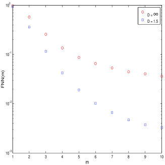
where is the slip deficit variance measured at equal sampling times years, is a time lag (an integer multiple of the common lag ), and is an embedding dimension. The optimal time lag, , has been chosen at the first minimum of the time-delayed mutual information as suggested in [12] and motivated in detail in [18]. The problem is to determine the optimal embedding dimension , for which the reconstruction by delay vectors provides an acceptable unfolding of the attractor so that the orbits composing the attractor are no longer crossing each other in the reconstructed phase space [1]. The practical solution is to look for false neighbors in the embedding phase space at a given value of [18]. To understand this concept, consider the situation that an dimensional delay reconstruction is an embedding, but an dimensional delay reconstruction is not. If the embedding dimension is too small to unfold the attractor, a small neighborhood will contain points that belong to different parts of the original attractor. Therefore, at a later time, the images of these points under the system’s dynamics will split onto different groups, depending on which part of the attractor the points are originally coming from. This lack of a unique location of all the images in dimensions is reflected in finding false neighbors, meaning that determinism is violated. When increasing , starting with small values, one can detect the minimal embedding dimension, , by finding no more false neighbors. Then, we can invoke the result of Sauer et al. [27] who showed that the attractor formed by in the embedding space is equivalent to the attractor in the unknown space in which the system is living if is larger than twice the box counting dimension, , of the attractor. Often, an embedding dimension is enough for unfolding the attractor. Therefore, the minimal embedding dimension sets the following bounds, , for the dimension of the attractor in the true phase space. Figure 5 shows that the percentage of false neighbors for the system falls under when the phase space embedding of the slip variance data reaches dimension seven. This behavior suggests a topological dimension in the true phase space between three and six. We note that the percentage of false neighbors is not completely reduced to zero. The explanation for this behavior is discussed in Section 6. To appreciate this result, we show for comparison in Fig. 5 the behavior of the system in the limit of no dynamic weakening. Even for an embedding dimension as high as ten, the percentage of false neighbors does not drop below , and is an order of magnitude larger than the percentage for the system at the same embedding dimension. This confirms our previous analysis and proves that in the limit of low dynamic weakening the system has high dimensional dynamics.
The foregoing analysis shows convincingly the deterministic structure of the large scale motions: for stochastic or very high dimensional dynamics the number of false neighbors will never effectively drop to zero. The low-dimension result is consistent with the embedding theorem [27] which asserts that it is not the dimension of the underlying true phase space that is important for the minimal dimension of the embedding space, but only the fractal dimension of the support of the invariant measure generated by the dynamics in the true phase space [18]. These results justify our earlier remarks that due to some collective behavior only a few dominant degrees of freedom remain and our conjecture that their dynamics is effectively deterministic.
Before addressing the problem of identifying these collective degrees of freedom, we would like to know if their dynamics is chaotic and, if so, what are the implications for their predictability. To answer this question we compute the maximal Lyapunov exponent. This exponent measures the exponential divergences of nearby trajectories and is an average of these local divergences over the whole data. A positive maximal Lyapunov exponent is a signature of chaos. Its computation is based on the algorithm described by Kantz and Schreiber [18] and uses the implementation provided in the publicly available software package TISEAN [16](all nonlinear time series algorithms described in this paper use the same excellent implementation). For a point of the time series in the embedding space, the algorithm determines all neighbors within a neighborhood of radius . Then, for each neighbor, we consider the distance and we read its evolution from the time series. If for all neighbors , then is the local divergence rate. The local divergence rate varies along the attractor and the true maximal Lyapunov exponent is an average over many reference points . Therefore, in practice we compute the average over the distances of all neighbors to the reference part of the trajectory as a function of the relative time . The logarithm of the average distance at time measures the effective expansion rate over the time span :
| (10) |
where the outer bracket denotes the averaging over the reference point , is the number of neighbors in , and the argument of the logarithm is the average local expansion rate. If vs exhibits a robust linear increase with identical slope for a range of values and for all larger than some minimum embedding value, then its slope is an estimate of the maximal Lyapunov exponent per time step [18]. Figure 6 shows three bundles of curves corresponding to three neighborhood sizes, , and , as can be seen for . Each bundle shows the behavior of the expansion rate for 6,7,8,9 and 10 and proves that the result is robust to changes in and does not depend on the embedding dimension when is large enough. Our estimate for the maximal Lyapunov exponent is . We can therefore conclude that the large scale motions have a positive maximal Lyapunov exponent and exhibit sensitive dependence on the initial conditions. Does this dependence sets a fundamental limitation to long-term forecasting? Two initially close trajectories will diverge exponentially in the phase space with a rate given by the largest Lyapunov exponent . Therefore, for any finite uncertainty in the initial conditions, we can forecast the future state of the system only up to a maximum time,
| (11) |
where is the accepted tolerance level. For the earthquake system, an approximate estimate for the predictability time is years. This result is disappointing and, due to expected model reconstruction errors, which might overshadow the uncertainty in the initial conditions, raises questions on the value of any forecasting endeavor. But this estimate is naive and holds only for infinitesimal perturbations and in nonintermittent systems. Generally, the predictability time is scale dependent [8] and can be much longer than the rough estimation . As we will shortly see, at the large length scale of interest for forecasting, a better estimation of the predictability time is years.
5 Proper Orthogonal Decomposition
The dynamics of the first and second order moments of the slip and stress fault fields provides an adequate description of the large scale motions. Unfortunately, their measurement poses very difficult problems: the stress field is not directly observable while the slip field requires the solution of an ill-posed inverse problem. Therefore, we propose an alternative analysis of the large scale motions based on the spatio-temporal strain patterns embedded in the surface deformation fields that can be accurately measured by InSAR and GPS observations [9]. Assuming uniform slip discontinuities over each rectangular cell, the components of the surface displacement vector are found to be [22],
| (12) |
where is the surface displacement in the direction at the observation point due to uniform unit slip on the fault cell located at . The space-time signal is obtained by simultaneous measurements of the surface displacements on a uniform rectangular grid which covers a surface area centered around the fault. For each surface deformation we compute an ensemble of snapshots, and , every years. The analysis of each deformation direction proceeds identically, therefore we will henceforth drop the deformation index . Since we are only interested in decomposing the dynamics of fluctuations, it is convenient to separate the flow into a time-independent mean and a fluctuating part, i.e.
| (13) |
where and indicates the ensemble average.
The identification of the active degrees of freedom in the surface deformation fields uses the Principal Orthogonal Decomposition (POD) [17]. The POD seeks an optimal representation (in the least square sense) for the members of the ensemble . It searches for generalized directions in the configuration phase space, such that most of the ensemble fluctuations will be directed along . Mathematically, this is achieved by maximizing the average projection of the ensemble onto , i.e.
| (14) |
where is the inner-product in the configuration space and the norm constraint, , is required for the maximum to be defined. The solution to this variational problem is given by the eigenfunctions of the following integral equation [17],
| (15) |
whose kernel is the two point correlation matrix of the ensemble, . There are at most eigenfunctions corresponding to the total number of degrees of freedom. The eigenvalues measure the mean square fluctuations of the ensemble in the directions defined by their corresponding eigenfunctions: . We can also think of as the average “energy” of the ensemble fluctuations projected onto the axis. Therefore, ranked in decreasing order of their eigenvalues, the eigenfunctions (sometimes called empirical eigenfunctions, coherent structures, or dominant modes) will identify the dominant directions in configuration space along which most of the fluctuations take place. The first four modes describing the predominant motions of the deformation field for system A with are shown in Fig. 7. The coherent, collective nature of the fluctuations represented by these modes is eloquently expressed by their spatial structure. The spatial coherence sharply decreases for the higher order modes (not shown). The modes probe the system at different scales, from the largest scales, captured by the most dominant modes, to the smallest scales, described by the higher order modes. This observation is hardly surprising, since for a translationally invariant system the POD modes are simply the Fourier modes [17].
The basis is optimal in the sense that any reduced representation of the form
| (16) |
describes typical members of the ensemble better than any linear representation of the same dimension in any other basis: the leading POD modes contain the greatest possible “energy” on average [17]. Therefore, due to the coherence and optimality of the POD basis, Eq. (16) provides the most efficient Euclidean (linear) embedding for the large scale motions of the system. Moreover, the modal coefficients are uncorrelated on average, i.e.
| (17) |
which reflects the fact that orthogonality in the embedding space, , is related to the statistical properties of the time series.
The choice of the embedding dimension is based on the computation of the cumulative normalized eigenvalue spectrum, , defined as:
| (18) |
The cumulative spectrum can help us define an effective POD embedding dimension by finding the minimum number of modes needed to capture some specific fraction of the total variance of the data:
| (19) |
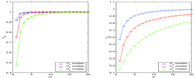
Figure 8 shows the cumulative normalized spectrum for each of the surface deformation modes. For system A (), in order to explain of the variance in the data sets we need only 2, 3, and 5 modes respectively. This is consistent with our earlier estimates of the embedding dimension. In contrast, for system B (), we need 9, 27, and 42 modes respectively.
It is important to realize that the POD modes carry no dynamic information. Reshuffling the ensemble of configurations - and, therefore, destroying the dynamic content hidden in their time ordering - produces the same POD modes. Therefore, in order to identify the dynamics of each POD mode we calculate the projections of the surface deformation fields onto the dominant deformation modes, i.e.,
| (20) |
This way, we generate a small number of modal time series that encode the evolution, interaction and dynamics of the spatial modes [17]. They encapsulate the projection of the system’s dynamics onto the -dimensional model space defined by Eq. (16).
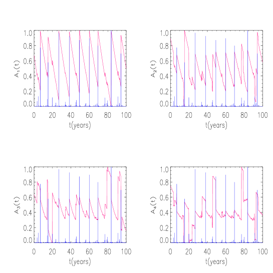
In Fig. 9 we represent the modal time series (red lines) corresponding to the first four spatial modes for fault system A. The blue lines describe the time evolution of the binned potency released (the total potency released over the time interval ). For the first time series, , the location in time of the amplitude jumps coincides with the time of large events (within the temporal resolution defined by ). Moreover, we can show that the size of the amplitude jumps is proportional with the size of the event, i.e. , where is the largest event in the ’th time interval. Therefore, if we can model the evolution of this mode, the time and size of the amplitude jumps will give us useful information about the time and size of the large earthquake events. Moreover, we notice that the higher order modes evolve on faster time scales, as is already noticeable from the faster decay of the temporal autocorrelations shown in Fig. 11.
The picture that emerges from this decomposition evolves gradually from the slow, coherent large scale motions, whose dynamics is captured by the most dominant POD modes, to the fast, incoherent small scale motions described by the higher order modes. In Section 7 7 Model Reconstruction and Short-Term Earthquake Forecasting we describe how a neural net can be used to process these time series in order to extract a low-dimensional nonlinear dynamic model with short-term predictive capabilities.
6 Geometry of the attractor in the POD basis
The POD modes provide an optimal basis for the phase space embedding expressed in Eq. (16). The phase space vectors in this reconstruction, , approximate the location of the system on the attractor at discrete time moments. Compared to the time-delay embedding, the POD basis unfolds the attractor with increased resolution as the embedding dimension increases. This property allows us to probe the structure of the attractor at different length scales by computing its correlation dimension. This measure was introduced by Grassberger and Procacia [14] to quantify the self-similarity of geometrical objects. It is based on the definition of the correlation sum for a collection of points in some vector space . This is the fraction of all possible pairs of points which are closer than a given in a particular norm. The basic formula is
| (21) |
where we use the maximum norm, , is the Heaviside step function, is the total number of data points, and is the total number of reference points. The sum counts the pairs whose distance is smaller than . Note that data points within a time window of any reference point are not included in the correlation sum. An appropriate choice of reduces the spoiling effect of autocorrelations from the correlation sums as suggested by Theiler [29]. In the limit of an infinite amount of data and small , the attractors of deterministic systems show power law scaling, i. e., , and we can define the correlation dimension by
| (22) |
For each embedding dimension , measures the local slopes of the correlation sum at different length scales ,
| (23) |
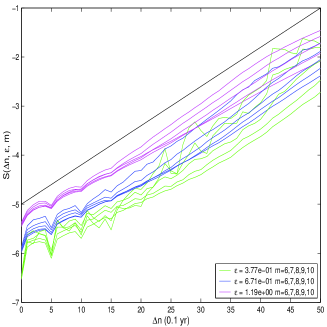
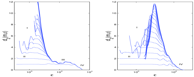
In Fig. 10. for system A on the left and B on the right, we show the dependence of for embedding dimensions . This plot allows the identification of a scaling range and estimation of the correlation dimension if such range occurs. This is reflected in the presence of a plateau in the dependence of which does not change much with embedding dimension when : the correlation sum probes the attractor at different length scale and tests for scale-invariance.
From the point of view of the physics involved, we distinguish four different types of behavior for at different regions of length scale [18]. For small and large (region I in Fig. 10) the lack of data points is the dominant feature and the values of are subject to large statistical fluctuations. If is of the order of the size of the entire attractor (region IV), no scale invariance can be expected. In between, we can distinguish two regions. In region II, at small length scales but good statistics due to the small embedding dimension, the reconstructed points reflect the low amplitude and high frequency dynamics generated by the small events. At these length scales the dynamics is high dimensional and the reconstructed points fill the entire phase space available, therefore we expect . Up to the embedding dimension this estimate is recovered in the limit For increased embedding dimension there are large statistical fluctuations due to the lack of neighbors.
For system A, in region III located at larger length scales between regions II and IV, the dynamics evolves on a low-dimensional self-similar attractor whose presence is detected by the plateau in the correlation dimension at . Note that for system A the scaling regime, , is not reachable. The breakdown of scaling at the smaller length scales is dynamic in nature and is not due to the lack of good statistics. The closer we look at the system, the more degrees of freedom become visible and the dimensionality of the dynamics is higher than our largest embedding dimension. This also explains why the percentage of false nearest neighbors never drops completely to zero with increased embedding dimension. On the same figure, within the range of embedding dimensions that were numerically accessible, system B shows no signature of a large scale dimension collapse, in dramatic contrast with the behavior of system A.
The length dependent dimensions lead us to conjecture that we observe different subsystems on different length scales. From the self-similar and low-dimensional structure at the large length scales the structure of system A attractor crosses-over to a high dimensional, stochastic like structure when probed at very small length scales. Our strategy for building a model with good forecasting skills should be obvious now. The underlying idea is to approximate the large scale motions of system A through a low-dimensional embedding into the subspace spanned by the most dominant POD modes and to extract a finite-dimensional model in the form of a set of ODEs of comparable dimension. Does a good nonlinear model for the large scale motions exists? The answer depends on how rapidly the small scale motions of the true system progress to reach the larger length scales. If this time is short, an effective model for the large scale motions might not exist. If the growth time is sufficiently long, the existence question is well posed and a model for the large scale motions might exist. To address this question we now proceed to the model reconstruction task.
7 Model Reconstruction and Short-Term Earthquake Forecasting
Using the POD decomposition we have identified a low-dimensional linear space in which system A evolves most of the time and we have reduced its dynamics to a small set of time series, , , describing the evolution of the system in this reduced linear space. We now face the problem of determining the underlying dynamical process from the information available in these time series. They are assumed to be governed by a nonlinear set of ODEs and our modeling approach relies on the ability to identify an approximate dimensional model,
| (24) |
that describes an explicit Euler approximation to the evolution and interaction of the spatial modes. To identify this nonlinear mapping we employ an artificial neural network (ANN). Generally, the neural network approach is used as a “black-box” tool in order to develop a dynamic model based only on observations of the system’s input-output behavior [23, 24]. In the learning process the network adjusts its internal parameters to minimize the squared error between the network output and the desired outputs. A typical learning method is the error back-propagation algorithm which is a first order gradient descent method [15].
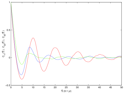
All reconstruction results described here refer to the dynamics of the surface deformation modes for model A with . We found it difficult to identify a simple model having the structure defined by Eq. (24). In order to improve the model forecasting skill it is useful to enlarge the structure of the model to include information about the past history of the modes. While the best model structure is still a subject of investigation, an analysis of the time patterns present in the modal evolution provides a partial understanding of this result. As Fig. 9 shows, one essential feature of the modal dynamics is the presence of two time scales: within each earthquake cycle there are intervals of slow and fast motions with detectable quasi-regular behavior. This is reflected in the two-point autocorrelation functions (Fig. 11) defined as
| (25) |
where the denotes the time average. The resulting plots exhibit oscillatory behavior with a slow amplitude decay over a longer time scale indicating that the system has two correlation time scales. We have observed that providing the ANN with information about these long-term correlations of the modal dynamics produces nonlinear models with increased forecasting skill. To include this information, we have modified the structure of the model in Eq. (24) and replaced the modal coefficients with time-delayed vectors ,
| (26) |
where is the delay and is the number of the time-delay intervals. Due to the presence in the modal dynamics of two different time scales, we have included both short, , as well as long time, , memory information in the time-delayed input vectors. The dimension of each time-delayed vector is . The ANN output then provides a prediction of the mode amplitude at time ,
| (27) |
based on input information describing the past mode histories.
The ANN is trained using a standard back-propagation algorithm [15]. When training succeeds, the ANN provides an approximate dynamical model (map) for the large scale motions of the fault. The map can be evaluated once to provide short term predictions or iterated to predict the long term fault dynamics. Besides the parameters describing the structure of the ANN (nonlinear transfer functions, number of layers and neurons in each layer), the model structure itself has many parameters (, , ) that can be adjusted in order to improve the model performance. Our goal is to find a good model describing the evolution of the first POD mode, whose dynamic discontinuities trace accurately the time and size of the large events. Information about the higher order modes and their past histories is only necessary to uniquely determine the state and model trajectory in its phase space. One of the best models found so far describes the evolution of the first two surface deformation modes: . For each spatial mode, a time-delayed vector with parameters and was used. Because the dimensionality of the input space, , is higher than our estimated embedding dimension, we have decided to perform a POD analysis of the ensemble of input vectors. This time, the POD decomposition performs the analysis of the dominant temporal patterns that are created by the modal dynamics. Similar to the spatial decomposition, we first compute the two point correlation matrix of the ensemble,
| (28) |
where denote the input modes, are the components of the time-delayed mode vectors, and is the average over the ensemble of input vectors. Due to the statistical independence of the modal coefficients, Eq. (17), the correlation matrix is to a good approximation block diagonal, i.e. for (any modal cross-correlations are due to finite size effects). The eigenvalues and normalized eigenvectors of the correlation matrix,
| (29) |
will now provide an optimal representation of the dynamics of the spatial modes:
| (30) |
where
| (31) |
We found that of the variance of the input ensemble (, and model) can be represented by the first six temporal modes . We have therefore chosen to approximate the input vectors presented to the ANN by their six dimensional POD projection onto the space spanned by the first six temporal eigenvectors. Denoting by this projection operator, the structure of the model has now become:
| (32) |
The best forecasting performance was obtained for an ANN with two hidden layers of 10 neurons each. The input to the network is the 6-dimensional projection and its 2-dimensional output, , is the model forecast for the first two mode amplitudes at the next time step. Because the large events have long recurrence times, the sequential selection of the training set will be dominated by input-output pairs that only express the quasi-linear behavior between two consecutive large events: the ANN will learn a linear model and will fail to forecast the intrinsically nonlinear large earthquake events. Therefore, we have designed the training set to include enough information describing the dynamics around the scarce large events. The modal time series were first rescaled to evolve in the interval . We then classified as large events all events in which the first mode has a jump larger than 0.05 in the rescaled units. Next, we chose a time window , and checked for the presence of a large event located at the center of this window, as it slides along the modal time series. If we found one, we called this a nonlinear window, and all the input-output pairs describing the evolution of the system inside this time window were included in the training set. For each nonlinear window, we have included training pairs from a linear window (a segment of the time series that did not have a large event). With this training set, the ANN adequately learned to model the linear as well as the nonlinear features of the dynamics.
Due to non-convexity of the error surface in the network parameter space, we train many ANNs starting from different initializations of the neuron weights. To avoid overfitting, the training process stops when the error on the validation set starts to increase - the validation sample is a subset of the training set which is not actually used in training. At the end of the training cycle each ANN provides a model for the system dynamics. To find the “best” model, we test the forecasting skill of each model realization using time series segments not included in the training or validation set. Starting from an initial configuration describing for each input mode the current amplitude and its past values, we iterate the ANN forward in time for a number of steps. At each time step the output of the network was used to update and reconstruct the ANN input for the next time step. Assuming perfect initial conditions this procedure provides a trajectory whose forecasting accuracy is controlled only by the imperfections of our model. However, the reconstructed model is always an imperfect one and perhaps a perfect model describing the large scale motions does not even exists. Moreover, the current state of the system in the model space is always obscured by observational uncertainty. To make things worse, our knowledge of the spatial modes themselves is limited by the finite size of the ensemble of surface deformations. For example, the accuracy of the two-point correlations cannot exceed , where is the size of the ensemble: when we have only observations of finite duration, the “true” modes, describing the large scale motions, will never be exactly known. How can we then evaluate the model forecasting skill? A detailed answer is beyond the scope of this paper and our goal here is only to show that despite all these difficulties, and many others not mentioned here, our imperfect models can provide stable and robust forecasts. Our remarks here follow Smith [28], to which we also refer for a clear discussion of uncertainty in initial conditions, model errors, ensemble verification, and predictability in general.
For nonlinear systems, uncertainty in the initial conditions severely limits the utility of single deterministic forecasts. Internal consistency requires that all nonlinear forecast should be ensemble forecasts [28]. In this approach to forecasting, a collection of initial conditions, each consistent with the observational uncertainty, are integrated forward in time. When the system evolves on an attractor, the selection of the initial conditions is far from trivial. For a perfect model ( a model that has the right dynamics and whose phase space is identical with the system’s phase space) the members of the ensemble should be restricted to live on the system’s invariant measure (attractor). Obviously, this is not a priori known. Unrestricted initial conditions, consistent only with the observational uncertainty, will extend into the full phase space and generate over-dispersive ensembles. When this is the case, the predicted probabilities will not match the relative frequencies as demonstrated by Gilmour [13]. Generally, all models, including ours, are imperfect and, therefore, a perfect ensemble and an accountable forecast method do not exists. Nevertheless, when the initial conditions are uncertain, ensemble forecasts are still required. A reasonable constraint would require the members of the ensemble to live on the projection of system’s invariant measure (attractor) into the model phase space, although this choice is not necessarily optimal or even unique [28].
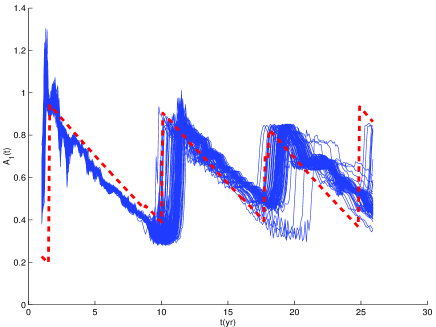
Assuming no a priori knowledge of the true attractor projected into the model phase space, we present in Fig. 12 an unconstrained ensemble of trajectories evolving under the dynamics of the ANN model. Each trajectory starts from a different initial state that contains small Gaussian perturbations from the exact initial conditions and is integrated forward in time for steps. We compare the ensemble evolution (blue lines) with the true evolution of the most dominant surface mode (red, thick line). The resulting ensembles of forecasts can be interpreted as a probabilistic prediction. The goal is to predict the time and the size of the jumps in the evolution of the first mode amplitude (which, as we have already discussed, corresponds to the time and size (potency) of large seismic events), and to estimate their forecast accuracy. Due to the time delay involved, the best time resolution of each trajectory cannot be in this case less than yr. As the fault evolves to the next time step, years later, we update the present state of the system and generate a new step ensemble forecast starting from this new state. This procedure is intended to incorporate the information about the system and its current state as is continuously generated by new observations.
Is clear from Fig. 12 that even though we lack a perfect model or an optimal ensemble, all members of the ensemble forecast the incoming sequence of large events. The forecast uncertainty of the ensemble grows very slowly showing long time reliability. The members of the ensemble spread out at a rate that depends on the local nonlinear structure of the model. This rate gives a local estimate of the stability of forecasts made in this region of the model’s state space. It also controls the time scale (predictability time) on which the ensemble members scatter along significantly different trajectories. We observe regions of large predictability time that coexist with regions of relatively short predictability time [8]. Significantly, the ANN has shown consistently the ability to improve its forecasting as the system approaches a large event. The predictability time is significantly larger than the microscopic expansion rate which is controlled by the maximal Lyapunov exponent. As hinted earlier, the predictability is scale dependent and the large scale motions are more predictable than the small scale motions.
The predictability also depends on the location of the system on its true underlying attractor. But unlike the growth of initial uncertainty in model phase space, the local nonlinear structure of the system’s attractor controls how rapidly the small scale motions, not included in our model, progress to reach the large length scales. This expansion rate defines how rapidly the truth, red line in Fig. 12, diverges from the best guess model trajectory. This is the trajectory starting from the true system state projected onto the model phase space. Of course, for the same model state there are infinitely many system states distinguishable only in their small length scale structure. Clearly, the accurate shadowing of the truth by the ensemble trajectories in Fig. 12, shows that growth of the small scale uncertainties does not severely limits the model forecasting skill. Their small growth rate makes possible the deterministic modeling of the large scale motions. It sets an upper bound for the model predictability time, which can be approached by improving the parametrization of the small scale dynamics.
8. Conclusions
We describe a conceptual framework for modeling and forecasting the evolution of a large strike-slip earthquake fault. The approach relies on the detection of spatio-temporal strain patterns embedded in the observable surface displacements: no detailed knowledge of the fault geometry, dynamics, or rheology is required. Rather than directly modeling the fault dynamics, we propose instead to model the dynamics of observable surface deformations, which are nonlinearly related to the original dynamics of the fault system.
The essence and novelty of the method lies in the discovery that the large length and time scales dynamics have a strong low-dimensional, deterministic component and are therefore amenable to representation by a deterministic model. We have also found that the large scale motions provide reliable forecasting information about the large seismic events. These two fundamental results set the stage for standard data processing and model reconstruction techniques. First, we identify the large scale motions with generalized directions (spatial modes) along which the dynamics has its largest fluctuations. Finding these directions is the natural task of the proper orthogonal decomposition applied to the ensemble of surface deformations generated during the evolution of the system. The most dominant spatial modes define the model phase space and provide an optimal embedding for the large scale dynamics of the system. Second, the model reconstruction consists in finding a nonlinear set of ODEs whose trajectory in model phase space approximates the system trajectory projected into the model phase space. This is a learning task that can be successfully accomplished by an artificial neural network.
The method relies on the existence of some separation between small and large length and time scales, and the physics responsible for this separation stems from the dynamic weakening used to model static/kinetic friction. We argue that in the presence of significant dynamic weakening the large scale dynamics defines the low-dimensional backbone of the system’s attractor. The small scale dynamics is practically indistinguishable from stochastic dynamics and evolves in a small neighborhood of the attractor backbone. Based on this geometric picture, we argue that the statistical properties of the small scale motions are determined by the larger-scale motions upon which they are superposed. In turn, the large scale motions depend on the statistical properties of the small scales. As pointed out by Lorenz [19], there remains uncertainties in the small scale statistics, and hence in their influence upon the larger scale. The predictability time of the large scale motions is controlled by the rapidity with which the small scales uncertainties progress to reach the very large scales. This sets an upper bound to the predictability time of any large scale model. Due to the robustness shown by the model ensemble forecast, we conclude that the intrinsic predictability time of the large scale dynamics is very long, perhaps of the order of 10-20 years. This is ultimately the reason behind the deterministic behavior of the large scale motions.
There are many difficult problems that are currently under investigation. For example, we presently study how robust the large scale behavior is to changes in the model parameters. Preliminary results confirm the controlling role of the dynamic weakening and show that the deterministic character of the large scale motions is robust to large changes in this parameter. We are also studying the effects of correlated heterogeneities, smooth brittle to ductile transitions, and continuous transition from static to kinetic friction. We do expect that all these effects are averaging out the small scale dynamics and strengthen the deterministic structure of the attractor. Probably, the most difficult problems to address are the construction of good models from short data observations and the problem of spatio-temporal chaos. In the last case, dimensions and Lyapunov exponents become intensive quantities and we want to understand how the method scales with the size of the fault system. The current paper is concerned primarily with developing a methodology and the obtained results are preliminary. Continuing studies along the directions of this work may have a significant impact on the earthquake predictability problem.
Acknowledgments
We express our gratitude to Yannis Kevrekidis for useful discussions and insightful suggestions. This research was performed under the auspices of the U. S. Department of Energy at LANL (LA-UR-02-6309) under contract W-7405-ENG-36 and LDRD-DR-2001501 (MA) and the National Earthquake Hazard Reduction Program of the USGS under grant 02HQGR0047 (YBZ).
References
- [1] Abarbanel, D. I. H., Analysis of Observed Chaotic Data (Springer-Verlag, NY, 1996).
- [2] Anghel, M., On the effective dimension and dynamic complexity of earthquake faults, submitted to Chaos, Solitons, and Fractals.
- [3] Ben-Zion, Y., and Rice, J. (1993), Earthquake failure sequences along a cellular fault zone in a three-dimensional elastic solid containing asperity and nonasperity regions, J. Geophys. Res. 98, 14109-14131.
- [4] Ben-Zion, Y. and Rice, J. R. (1995), Slip patterns and earthquake populations along different classes of faults in elastic solids, J. Geophys. Res. 100, 12959-12983.
- [5] Ben-Zion, Y. (1996), Stress, Slip, and Earthquakes in Models of Complex Single-Fault Systems Incorporating Brittle and Creep Deformations, J. Geophys. Res. 101, 5677-5706.
- [6] Ben-Zion, Y., Eneva, M., and Liu, Y. (2003), Large Earthquake Cycles and Intermittent Criticality On Heterogeneous Faults Due To Evolving Stress and Seismicity, J. Geophys. Res. in press.
- [7] Ben-Zion, Y., Key Formulas in Earthquake Seismology, in International Handbook of Earthquake and Engineering Seismology, Part B (Academic Press, 2003).
- [8] Boffetta, G., Cencini, M., Falcioni, M., Vulpiani, A. (2002), Predictability: a way to characterize complexity, Phys. Rep. 356, 367-474.
- [9] Burgmann, R., Rosen, P. A., and Fielding, E. J. (2000), Synthetic aperture radar interferometry to measure Earth’s surface topography and its deformation, Annu. Rev. Earth Planet. Sci. 28, 169-209.
- [10] Chinnery, M. (1963), The stress changes that accompany strike-slip faulting, Bull. Seismol. Soc. Amer. 53, 921-932.
- [11] Fisher, D. S., Dahmen, K., Ramanathan, S., and Ben-Zion, Y. (1997), Statistics of earthquakes in simple models of heterogeneous faults, Phys. Rev. Let. 78, 4885-4888.
- [12] Fraser, A., and Swiney, H. L. (1986), Independent coordinates for strange attractors from mutual information, Phys. Rev. A 33, 1134-1140.
- [13] Gilmour, I. (1998), Nonlinear model evolution: -shadowing, probabilistic prediction and weather forecasting, D. Phil. Thesis, Oxford University.
- [14] Grassberger P., and Procacia I. (1983), Measuring the strangeness of strange attractors, Physica D 9, 189-208.
- [15] Haykin, S., Neural Networks: A Comprehensive Foundation (Prentice Hall, NJ 1999).
- [16] Hegger, R., Kantz, H., and Schreiber, T. (1999), Practical implementation of nonlinear time series methods: The TISEAN package, CHAOS 9, 413-435.
- [17] Holmes, P., Lumley, J. L., and Berkooz, G., Turbulence, Coherent Structures, Dynamical systems and Symmetry (Cambridge University Press, Cambridge 1996).
- [18] Kantz, H., and Schreiber, T., Non-linear time Series Analysis (Cambridge University Press, Cambridge 1997).
- [19] Lorenz, E. N. (1969), The predictability of a flow which possesses many scales of motion, Tellus 21, 289-307.
- [20] Madariaga, R. (1976), Dynamics of an expanding circular fault, Bull. Seismol. Soc. Am. 66, 639-666.
- [21] Manneville, M., Dissipative Structures and Weak Turbulence (Academic Press, CA 1990).
- [22] Okada, Y. (1985), Surface deformations due to shear and tensile faults in a half-space, Bull. Seism. Soc. Am. 75, 1135-1154.
- [23] Rico-Martinez, R., Krischer, K., Kevrekidis, I. G., Kube M. C., and Hudson, J. L. (1992), Discrete- vs. continuous-time nonlinear signal processing of Cu electrodissolution data, Chem. Eng. Comm. 118, 25-48.
- [24] Rico-Martinez, R., Kevrekidis, I. G., and Krischer, K., Nonlinear system identification using neural networks: dynamics and instabilities, In Neural networks for chemical engineers (ed. Bulsari. A. B., Elsevier Science 1995) pp. 409-442.
- [25] Rundle, J. B., Klein, W., Tiampo, K. F., and Gross, S. (2000), Linear pattern dynamics in nonlinear threshold systems, Phys. Rev. E 61, 2418-2431.
- [26] Sammis, C. G., and Sornette, D. (2002), Positive feedback, memory, and the predictability of earthquakes, PNAS 99, 2501-2508.
- [27] Sauer T., Yorke, J. A., and Casdagli, M. (1991) Embedology, J. Stat. Phys. 65, 579-616.
- [28] Smith, L., Disentangling uncertainty and error: On the predictability of nonlinear systems, In Nonlinear dynamics and statistics (ed. Mees A., Birkhuser 2000) pp. 31-64.
- [29] Theiler, J. (1990), Estimating fractal dimension, J. Opt. Soc. Am. A 7, 1055-1073.
- [30] Wesnousky, S. G. (1994), The Gutenberg-Richter or characteristic earthquake distribution, which is it?, Bull. Seism. Soc. Am. 84, 1940-1959.
Captions
-
Fig. 1
Schematic evolution of the stress and slip for an individual fault cell. The parameters that describe the static/kinetic friction law are: static strength, , dynamic strength, , and arrest stress, . The time dependent failure strength of the cell, , equals the static strength if the cell has not slipped yet and is adjusted to its dynamic value when the cell fails (from [3]).
-
Fig. 2
A years evolution of the potency released by two fault systems. Results for system A, with small dynamic overshoot are on the left and for system B, with large dynamic overshoot (and no dynamic weakening) are on the right. System A exhibits quasi-regular seismic cycles associated with the large events. There is no detectable structure in the evolution of seismicity in system B.
-
Fig. 3
Time evolution of the average slip deficit (left) and its variance (right) for the (blue line) and (red line) fault systems.
-
Fig. 4
Log-log frequency-size histogram plots for the system (blue squares) and the system (red circles). The earthquake size is measured by its potency and the histograms use equal bins of size 100 in potency units ().
-
Fig. 5
The fraction of false nearest neighbors (FNN) as a function of the embedding dimension . Compared to model B (), there is a dramatic decrease in the number of FNN for model A (), as the dimension of the embedding phase space is increased. This suggests that a low-dimensional deterministic dynamics is a good approximation for the large scale dynamics of the fault.
-
Fig. 6
Estimates of the maximal Lyapunov exponent from the slip deficit variance time series data, , for the model. The logarithm of the stretching factor is computed for three different neighborhood sizes, , and embedding dimensions. The robust linear behavior of reflects the underlying determinism of the data and its slope is an estimate of the maximal Lyapunov exponent, (the straight line has slope and the unit of time is years).
-
Fig. 7
The first four POD spatial modes of the surface deformation field for fault system A with dynamic overshoot . These modes define, in decreasing order of their eigenvalues, generalized deformation directions which support most of the variance produced by the dynamics of surface fluctuations. The coherent, collective nature of the modes is reflected in their overall shape.
-
Fig. 8
Cumulative normalized eigenvalue spectrum for each of the surface deformation modes for system A on the left and B on the right - only the first 20 POD modes are shown. In order to explain of the variance in the data sets for system A we need only 2, 3, and 5 modes respectively. In contrast, for system B we need 9, 27, and 42 modes. Generally, the surface deformations along the strike direction, , have the most efficient POD description.
-
Fig. 9
Modal time series (red lines) describing the evolution of the first four spatial modes shown in Fig. 7. This time dependence is determined by projecting the surface deformation onto each POD mode every years. The blue lines describe the time evolution of the cumulative potency released over each year interval. Note the correlations between the time intervals of high potency released and the discontinuities present in the temporal modes.
-
Fig. 10
Local slopes of the correlation sum for the multivariate time series describing the evolution of systems A (on the left) and B (on the right) for embedding dimensions . For system A (), we detect the emergence of a scaling region around , suggesting a correlation dimension and self-similar geometry of the attractor at the large length scales. This behavior breaks down when the attractor is probed at smaller length scales where the dynamics is high dimensional. Within the same range of embedding dimensions, system B () shows no signature of a large scale dimension collapse.
-
Fig. 11
The temporal autocorrelations of the first three modes of the deformation field in model (mode 1 red line, mode 2 blue line, and mode 3 green line). The short-term oscillatory behavior and the slow long-term amplitude decay reveal the presence of two correlation time scales. The oscillations become faster and the long-term coherence decreases rapidly for the higher order modes.
-
Fig. 12
Model ensemble forecast for the evolution of the first mode (coordinate In model phase space) as predicted by the iterated ANN (blue lines). Each trajectory of the ensemble starts from a different initial condition and is integrated forward in time for 250 steps. Each ensemble trajectory evolves into the model phase space, while the red dashed line represents the true trajectory of the system projected onto the first coordinate of the model phase space (mode one). The ensemble is consistent with an arbitrary Gaussian, initial observational uncertainty, but its members do not live on the projection of the true system’s attractor into the model phase space. Nevertheless, all members of the ensemble consistently forecast the incoming sequence of large events, proving the long term forecasting reliability. We also notice a systematic bias in estimating the time to the next large event.