[physics/0305097] Chapter 1 Computational Techniques for Simulating Light Propagation in High-Energy Neutrino Telescopes

Abstract

To maximize the accuracy of background simulation and event reconstruction, high-energy neutrino telescopes require detailed knowledge of light propagation over a large volume of detection medium. If light scattering and absorption lengths in the medium are of the same scale as the detector size, this problem can only be handled numerically. Any inhomogeneity of optical properties in the medium further complicates the problem, requiring large computational resources. We present a treatment based on combining ray-tracing Monte Carlo and neural network techniques which offers a reasonable compromise between solution accuracy, computer memory and CPU usage.

1. Introduction

Any high-energy neutrino telescope has to reject an overwhelming background produced by cosmic-ray-generated atmospheric muons before any neutrino signal can be extracted. The background data simulation needs to faithfully reproduce all known classes of background events, while the event reconstruction should be accurate enough to allow their separation from the expected signal. For these tasks, correctly describing the photon transport in the detector is crucial.

An important requirement for a functional neutrino telescope is that its size should be smaller than the volume at which photon transport through its detection medium can be considered diffusive, but also large enough to have reasonable signal collection area. In a medium where absorption dominates over scattering, like deep ocean or lake sites, the light transport problem can be solved analytically if scattering is neglected or treated as a correction. In the regime where scattering and absorption distances are similar, as is the case for AMANDA [4], the problem has to be tackled numerically. To satisfy the above requirement, the numerical solutions have to be tabulated over large volumes.

In this report we describe numerical techniques that were used to produce satisfactory results for use in AMANDA in terms of solution accuracy and ease of implementation into computational structure. The same approach can be easily adapted to any other detector facing similar problems.

2. Photon table generation

The distribution of time dependent photon fluxes around a light source is generated by a photon transport Monte Carlo simulation which has been optimized for numerical accuracy and speed of execution [3]. The photon transport is done in a fashion analogous to the ray-tracing technique employed in computer graphics design. The main difference is that instead of recording the “illumination” of the predefined set of objects, the entire photon propagation volume is subdivided into cells which independently record time-dependent photon flux. This method allows a rapid collection of large photon statistics: $\sim\!10^{6}\;\gamma$ /CPU hour on 650 MHz Pentium III.

Since the detector medium is considered not to have boundaries, light scattering is caused only by impurities contained within the ice, which also dominate the absorption in the visible wavelength range. The depth-dependent concentration and composition of these impurities has been studied and a model for the description of optical properties of ice in AMANDA as a function of depth has been developed [5]. The inhomogeneity of optical properties of ice partially breaks the translational and rotational symmetries of the problem and requires that each light emission point be treated separately.

In AMANDA, the instrumentation is surrounded by columns of re-frozen ice enriched in microscopic air-bubbles. This ice occupies only a very small fraction of the detection volume, and will only affect photon distribution near the detection point. Thus it can be treated as a perturbation to the directional sensitivity of the light detectors instead of being incorporated into the photon transport simulation.

Refer to caption — Fig. 1.: Logarithm of the photon fluence $\mathcal{F}$ for points along the particle track $z^{\prime}$ at distances $\rho$ = 0, 3, 12, 27, 48, 75, 108, 147, 192 and 243 meters from the track – top to bottom.

For the purpose of detector response simulation, photon distributions resulting from all relevant source depths and orientations have to be simulated. In the case of AMANDA, this covers $\sim$ 700 meters of depth and 4 $\pi$ of solid angle. Combining the sizes of tables describing the photon flux around each of these sources, the overall size of the photon table set becomes very large; $\sim$ 1 GB even for a very coarse binning. Increasing the quality (for improved simulation accuracy) or the number (for larger detectors [1]) of tables quickly becomes prohibitive if one should hope to use most readily-available computational resources.

Possible solutions would be to either segment detector simulation in such a way that only a subset of all tables would be needed at any given time, or to reduce the memory needed to describe the content of each table. To pursue the second option, we have chosen to use neural networks to make a model-free fit to the tables and use the network output in the detector simulation.

3. Neural Network (NN) implementation

The photon flux is stored in tables as photon fluence $\mathcal{F}_{ij}=f(\mathbf{r}_{\mathrm{src},i},\mathbf{r}_{j})$ at a point $\mathbf{r}_{j}$ due to a source at $\mathbf{r}_{\mathrm{src},i}$ , and as a normalized time profile of the flux $P_{ijk}=g(\mathbf{r}_{\mathrm{src},i},\mathbf{r}_{j},t_{k})$ where $t_{k}$ is time delay with respect to an unscattered photon from the same source. We now represent the functions $\mathcal{F}$ and $P$ by multi-layer perceptron (MLP) neural networks [2] with as many input nodes as there are coordinates, a single output node for the function value, and a number of hidden nodes to be determined. The table coordinates and stored values are used to create neural net training patterns.

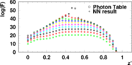
The photon tables map 5 spatial coordinates to a fluence which can extend over 20 orders of magnitude in the case of AMANDA. This is beyond the dynamic range of a neural net, so the logarithm of the fluence is fitted. All input coordinates are rescaled on [0,1] range. In order to find a suitable net architecture, we consider first a fluence projection onto the dimension along which the function shows the most features. Hidden nodes and layers are added/removed until we find a satisfactory agreement between the neural net output and the tabulated value expressed in the linear fluence units. After this, input nodes are added one at a time for the additional, smoother dimensions. The hidden layer configuration can be modified if necessary, but we usually find that the additional links from the new input nodes can handle the additional dimensions. We train the net until the difference between the network output and the desired function values stabilizes. Figure LABEL:008856-1:AmpFit shows the excellent network response to the fluence training for the light emitted by a short particle-track segment.

Fitting delay tables follows the same method as the fluence tables, but with one additional input coordinate. In the detector simulation, one wishes to randomly sample $P$ in order to generate timing response of the detector. To do this, one is interested in the integrated and time-inverted function of $P$ , $t=h(\int_{0}^{t}\!Pdt^{\prime})$ , which can be easily expressed in neural net formulation. If the function $\int_{0}^{t}\!Pdt^{\prime}$ is not one-to-one, we exclude the flat part of the function from the fit, and if due to binning effects $t\neq 0$ for all values of $\int_{0}^{t}\!Pdt^{\prime}$ , we add a pattern $(\int_{0}^{t}\!Pdt^{\prime}=0,t=0)$ to make the function on-to.

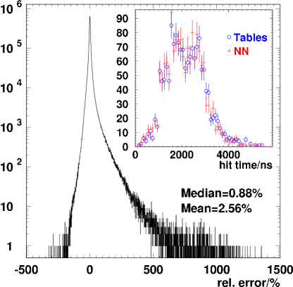
To avoid biasing the network to the order in which patterns are stored, they are shuffled before network training. For network construction and training we use the SNNS package [6]. In the case of fluence tables, all patterns fit into a standard computer memory and can be used in a single training session. In the case of delay tables, only $\sim$ 10% of patterns fit into memory, so a random subsample is used. The network’s interpolation capability (Fig. LABEL:008856-1:TimeExample) ensures that the patterns not used for training are nevertheless accurately reproduced within 2.6% (Fig. LABEL:008856-1:TimeFit). Large relative-error tails, seen in Fig. LABEL:008856-1:TimeFit, occur only for very short time-delays and produce no adverse effect on application of net output.

4. Results

After training, the network can be used in the standard detector response simulator. To check the accuracy of the net, we compare events simulated using the direct table lookup to events simulated using the neural net representation. It is found that simulated hit-amplitude and hit-time distributions are in good agreement (inset Fig. LABEL:008856-1:TimeFit). The memory reduction factor achieved is $\sim$ 1000 for the fluence tables and $\sim$ 0.5 $\times 10^{6}$ for the timing tables. We observe no CPU runtime increase due to NN evaluation.

We would like to thank K. Woschnagg, S. Hundertmark, L. Gerhardt, and M. Kowalski for help and advice.

References

1. Ahrens J. 2003, ArXiv: astro-ph/0305196

2. Haykin S. 1999, in “Neural Networks: A Comprehensive Foundation” (Prentice-Hall, New Jersey)

3. Miočinović P. 2001, Ph.D. thesis, http://area51.berkeley.edu/manuscripts

4. Wagner W. et al., these proceedings

5. Woschnagg K. 1999, in Proc. 26^th ICRC (IUPAP, Salt Lake City), Vol. 2, 200

6. Zell A. et al. 1995, SNNS User Manual, IPVR, Univ. of Stuttgart, Germany