Empirical Distributions of Log-Returns:
between the Stretched Exponential and the Power Law?

Abstract

A large consensus now seems to take for granted that the distributions of empirical returns of financial time series are regularly varying, with a tail exponent $b$ close to $3$. First, we show by synthetic tests performed on time series with time dependence in the volatility with both Pareto and Stretched-Exponential distributions that for sample of moderate size, the standard generalized extreme value (GEV) estimator is quite inefficient due to the possibly slow convergence toward the asymptotic theoretical distribution and the existence of biases in presence of dependence between data. Thus it cannot distinguish reliably between rapidly and regularly varying classes of distributions. The Generalized Pareto distribution (GPD) estimator works better, but still lacks power in the presence of strong dependence. Then, we use a parametric representation of the tail of the distributions of returns of 100 years of daily return of the Dow Jones Industrial Average and over 1 years of $5$-minutes returns of the Nasdaq Composite index, encompassing both a regularly varying distribution in one limit of the parameters and rapidly varying distributions of the class of the Stretched-Exponential (SE) and Log-Weibull distributions in other limits. Using the method of nested hypothesis testing (Wilks’ theorem), we conclude that both the SE distributions and Pareto distributions provide reliable descriptions of the data and cannot be distinguished for sufficiently high thresholds. However, the exponent $b$ of the Pareto increases with the quantiles and its growth does not seem exhausted for the highest quantiles of three out of the four tail distributions investigated here. Correlatively, the exponent $c$ of the SE model decreases and seems to tend to zero. Based on the discovery that the SE distribution tends to the Pareto distribution in a certain limit such that the Pareto (or power law) distribution can be approximated with any desired accuracy on an arbitrary interval by a suitable adjustment of the parameters of the SE distribution, we demonstrate that Wilks’ test of nested hypothesis still works for the non-exactly nested comparison between the SE and Pareto distributions. The SE distribution is found significantly better over the whole quantile range but becomes unnecessary beyond the $95\%$ quantiles compared with the Pareto law. Similar conclusions hold for the log-Weibull model with respect to the Pareto distribution. Summing up all the evidence provided by our battery of tests, it seems that the tails ultimately decay slower than any SE but probably faster than power laws with reasonable exponents. Thus, from a practical view point, the log-Weibull model, which provides a smooth interpolation between SE and PD, can be considered as an appropriate approximation of the sample distributions. We finally discuss the implications of our results on the “moment condition failure” and for risk estimation and management.

key-words: Extreme-Value Estimators, Non-Nested Hypothesis Testing, Pareto distribution, Weibull distribution

1 Motivation of the study

The determination of the precise shape of the tail of the distribution of returns is a major issue both from a practical and from an academic point of view. For practitioners, it is crucial to accurately estimate the low value quantiles of the distribution of returns (profit and loss) because they are involved in almost all the modern risk management methods. From an academic perspective, many economic and financial theories rely on a specific parameterization of the distributions whose parameters are intended to represent the “macroscopic” variables the agents are sensitive to.

The distribution of returns is one of the most basic characteristics of the markets and many papers have been devoted to it. Contrarily to the average or expected return, for which economic theory provides guidelines to assess them in relation with risk premium, firm size or book-to-market equity (see for instance FF96), the functional form of the distribution of returns, and especially of extreme returns, is much less constrained and still a topic of active debate. Naively, the central limit theorem would lead to a Gaussian distribution for sufficiently large time intervals over which the return is estimated. Taking the continuous time limit such that any finite time interval is seen as the sum of an infinite number of increments thus leads to the paradigm of log-normal distributions of prices and equivalently of Gaussian distributions of returns, based on the pioneering work of Bachelier00 later improved by Samuelson. The log-normal paradigm has been the starting point of many financial theories such as Markovitz59’s portfolio selection method, Sharpe64’s market equilibrium model or BS73’s rational option pricing theory. However, for real financial data, the convergence in distribution to a Gaussian law is very slow [Campbell, BP00, for instance], much slower than predicted for independent returns. As table 1 shows, the excess kurtosis (which is zero for a normal distribution) remains large even for monthly returns, testifying (i) of significant deviations from normality, (ii) of the heavy tail behavior of the distributions of returns and (iii) of significant dependences between returns [Campbell].

Another idea rooted in economic theory consists in invoking the “Gibrat principle” [Simon] initially used to account for the growth of cities and of wealth through a mechanism combining stochastic multiplicative and additive noises [LSR96, SC97, Biham98, DS98] leading to a Pareto distribution of sizes [Champenowne, Gabaix]. Rational bubble models a la Blanchardwat can also be cast in this mathematical framework of stochastic recurrence equations and leads to distribution with power law tails, albeit with a strong constraint on the tail exponent [LuxSor, MalSor]. These frameworks suggest that an alternative and natural way to capture the heavy tail character of the distributions of returns is to use distributions with power-like tails (Pareto, Generalized Pareto, stable laws) or more generally, regularly-varying distributions [BGT87] , the later encompassing all the former.

In the early 1960s, Mandelbrot63 and Fama65 presented evidence that distributions of returns can be well approximated by a symmetric Lévy stable law with tail index $b$ about $1.7$. These estimates of the power tail index have recently been confirmed by MRP98, and slightly different indices of the stable law ($b=1.4$) were suggested by MS95 MS95,MS00. On the other hand, there are numerous evidences of a larger value of the tail index $b\cong 3$ [Longin96, GDDMOP97, GMAS98, GMAS98_2, Plerouetal99, MDP98, Farmer99, Lux00]. See also the various alternative parameterizations in term of the Student distribution [Blattberg, kon], or Pearson type-VII distributions [Naga], which all have an asymptotic power law tail and are regularly varying. Thus, a general conclusion of this group of authors concerning tail fatness can be formulated as follows: tails of the distribution of returns are heavier than a Gaussian tail and heavier than an exponential tail; they certainly admit the existence of a finite variance ($b>2$), whereas the existence of the third (skewness) and the fourth (kurtosis) moments is questionable.

These apparent contradictory results actually do not apply to the same quantiles of the distributions of returns. Indeed, MS95 have shown that the distribution of returns can be described accurately by a Lévy law only within a limited range of perhaps up to 4 standard deviations, while a faster decay of the distribution is observed beyond. This almost-but-not-quite Lévy stable description explains (in part) the slow convergence of the returns distribution to the Gaussian law under time aggregation [Sorbook]. And it is precisely outside this range where the Lévy law applies that a tail index of about three have been estimated. This can be seen from the fact that most authors who have reported a tail index $b\cong 3$ have used some optimality criteria for choosing the sample fractions (i.e., the largest values) for the estimation of the tail index. Thus, unlike the authors supporting stable laws, they have used only a fraction of the largest (positive tail) and smallest (negative tail) sample values.

It would thus seem that all has been said on the distributions of returns. However, there are dissenting views in the literature. Indeed, the class of regularly varying distributions is not the sole one able to account for the large kurtosis and fat-tailness of the distributions of returns. Some recent works suggest alternative descriptions for the distributions of returns. For instance, GJ98 claim that the distribution of returns on the French stock market decays faster than any power law. contdub have proposed to use exponentially truncated stable distributions, Barndorff, Eberlein and Prause have respectively considered normal inverse Gaussian and (generalized) hyperbolic distributions, which asymptotically decay as $x^{\alpha}\cdot\exp(-\beta x)$, while LS99 suggest to fit the distributions of stock returns by the Stretched-Exponential (SE) law. These results, challenging the traditional hypothesis of power-like tail, offer a new representation of the returns distributions and need to be tested rigorously on a statistical ground.

A priori, one could assert that Longin96’s results should rule out the exponential and Stretched-Exponential hypotheses. Indeed, his results, based on extreme value theory, show that the distributions of log-returns belong to the maximum domain of attraction of the Fréchet distribution, so that they are necessarily regularly varying power-like laws. However, his study, like almost all others on this subject, has been performed under the assumption that (1) financial time series are made of independent and identically distributed returns and (2) the corresponding distributions of returns belong to one of only three possible maximum domains of attraction. However, these assumptions are not fulfilled in general. While Smith85’s results indicate that the dependence of the data does not constitute a major problem in the limit of large samples, we shall see that it can significantly bias standard statistical methods for samples of size commonly used in extreme tails studies. Moreover, Longin’s conclusions are essentially based on an aggregation procedure which stresses the central part of the distribution while smoothing the characteristics of the tail, which are essential in characterizing the tail behavior.

In addition, real financial time series exhibit GARCH effects [Bollerslev86, BEN94] leading to heteroscedasticity and to clustering of high threshold exceedances due to a long memory of the volatility. These rather complex dependent structures make difficult if not questionable the blind application of standard statistical tools for data analysis. In particular, the existence of significant dependence in the return volatility leads to the existence of a significant bias and an increase of the true standard deviation of the statistical estimators of tail indices. Indeed, there are now many examples showing that dependences and long memories as well as nonlinearities mislead standard statistical tests [AEL99, GT99, for instance]. Consider the Hill’s and Pickand’s estimators, which play an important role in the study of the tails of distributions. It is often overlooked that, for dependent time series, Hill’s estimator remains only consistent but not asymptotically efficient [RLdH98]. Moreover, for financial time series with a dependence structure described by a IGARCH process, KP97 have shown that the standard deviation of Hill’s estimator obtained by a bootstrap method can be seven to eight time larger than the standard deviation derived under the asymptotic normality assumption. These figures are even worse for Pickand’s estimator.

The question then arises whether the many results and seemingly almost consensus obtained by ignoring the limitations of usual statistical tools could have led to erroneous conclusions about the tail behavior of the distributions of returns. Here, we propose to investigate once more this delicate problem of the tail behavior of distributions of returns in order to shed new lights . To this aim, we investigate two time series: the daily returns of the Dow Jones Industrial Average (DJ) Index over a century (kindly provided by Prof. H.-C. G. Bothmer) and the five-minutes returns of the Nasdaq Composite index (ND) over one year from April 1997 to May 1998 obtained from Bloomberg. These two sets of data have been chosen since they are typical of the data sets used in most previous studies. Their size (about $20,000$ data points), while significant compared with those used in investment and portfolio analysis, is however much smaller than recent data-intensive studies using ten of millions of data points [GMAS98, GMAS98_2, Plerouetal99, matia, mizumo].

First, we show by synthetic tests performed on time series with time dependence in the volatility with both Pareto and Stretched-Exponential distributions that for sample of moderate size, the standard generalized extreme value (GEV) estimator is quite inefficient due to the possibly slow convergence toward the asymptotic theoretical distribution and the existence of biases in presence of dependence between data. Thus it cannot distinguish reliably between rapidly and regularly varying classes of distributions. The Generalized Pareto distribution (GPD) estimator works better, but still lacks power in the presence of strong dependence. Then, we use a parametric representation of the tail of the distributions of returns of our two time series, encompassing both a regularly varying distribution in one limit of the parameters and rapidly varying distributions of the class of the Stretched-Exponential (SE) and Log-Weibull distributions in other limits.

Using the method of nested hypothesis testing (Wilks’ theorem), our second conclusion is that none of the standard parametric family distributions (Pareto, exponential, stretched-exponential, incomplete Gamma and Log-Weibull) fits satisfactorily the DJ and ND data on the whole range of either positive or negative returns. While this is also true for the family of stretched exponential and the log-Weibull distributions, these families appear to be the best among the five considered parametric families, in so far as they are able to fit the data over the largest interval. For the high quantiles (far in the tails), both the SE distributions and Pareto distributions provide reliable descriptions of the data and cannot be distinguished for sufficiently high thresholds. However, the exponent $b$ of the Pareto increases with the quantiles and its growth does not seem exhausted for the highest quantiles of three out of the four tail distributions investigated here. Correlatively, the exponent $c$ of the SE model decreases and seems to tend to zero

Based on the discovery presented here that the SE distribution tends to the Pareto distribution in a certain limit such that the Pareto (or power law) distribution can be approximated with any desired accuracy on an arbitrary interval by a suitable adjustment of the parameters of the SE distribution, we demonstrate that Wilks’ test of nested hypothesis still works for the non-exactly nested comparison between the SE and Pareto distributions. The SE distribution is found significantly better over the whole quantile range but becomes unnecessary beyond the $95\%$ quantiles compared with the Pareto law. The log-Weibull model seems to be a good candidate since it provides a smooth interpolation between the SE and PD models. The log-Weibull distribution is at least as good as the Stretched-Exponential model, on a large range of data, but again, the Pareto distribution is ultimately the most parsimonious.

Collectively, these results suggest that the extreme tails of the true distribution of returns of our two data sets are fatter that any stretched-exponential, strictly speaking -i.e., with a strickly positive fractional exponent- but thinner than any power law. Thus, notwithstanding our best efforts, we cannot conclude on the exact nature of the far-tail of distributions of returns.

As already mentioned, other works have proposed the so-called inverse-cubic law ($b=3$) based on the analysis of distributions of returns of high-frequency data aggregated over hundreds up to thousands of stocks. This aggregating procedure leads to novel problems of interpretation. We think that the relevant question for most practical applications is not to determine what is the true asymptotic tail but what is the best effective description of the tails in the domain of useful applications. As we shall show below, it may be that the extreme asymptotic tail is a regularly varying function with tail index $b=3$ for daily returns, but this is not very useful if this tail describes events whose recurrence time is a century or more. Our present work must thus be gauged as an attempt to provide a simple efficient effective description of the tails of distribution of returns covering most of the range of interest for practical applications. We feel that the efforts requested to go deeper in the tails beyond the tails analyzed here, while of great interest from a scientific point of view to potentially help unravel market mechanisms, may be too artificial and unreachable to have significant applications.

The paper is organized as follows.

The next section is devoted to the presentation of our two data sets and to some of their basic statistical properties, emphasizing their fat tailed behavior. We discuss, in particular, the importance of the so-called “lunch effect” for the tail properties of intra-day returns. We then obtain the well-known presence of a significant temporal dependence structure and study the possible non-stationary character of these time series.

Section 3 attempts to account for the temporal dependence of our time series and investigates its effect on the determination of the extreme behavior of the tails of the distribution of returns. In this goal, we build a simple long memory stochastic volatility process whose stationary distributions are by construction either asymptotically regularly varying or exponential. We show that, due to the time dependence on the volatility, the estimation with standard statistical estimators may become unreliable due to the significant bias and increase of the standard deviation of these estimators. These results justify our re-examination of previous claims of regularly varying tails.

To fit our two data sets, section 4 proposes two general parametric representations of the distribution of returns encompassing both a regularly varying distribution in one limit of the parameters and rapidly varying distributions of the class of stretched exponential and log-Weibull distributions in another limit. The use of regularly varying distributions have been justified above. From a theoretical view point, the class of stretched exponentials is motivated in part by the fact that the large deviations of multiplicative processes are generically distributed with stretched exponential distributions [FrischSor]. Stretched exponential distributions are also parsimonious examples of the important subset of sub-exponentials, that is, of the general class of distributions decaying slower than an exponential. This class of sub-exponentials share several important properties of heavy-tailed distributions [EKM97], not shared by exponentials or distributions decreasing faster than exponentials. The interest of the log-Weibull comes from the smooth interpolation it provides between any Stretched-Exponential and any Pareto distributions.

The descriptive power of these different hypotheses are compared in section 5. We first consider nested hypotheses and use Wilks’ test to compare each distribution (Pareto, Exponential, Gamma and Stretched Exponential) with the most general parameterization which encompasses all of them. It appears that both the stretched-exponential and the Pareto distributions are the best and most parsimonious models compatible with the data with a slight advantage in favor of the stretched exponential model. Then, in order to directly compare the descriptive power of these two models, we use the important remark that, in a certain limit where the exponent $c$ of the stretched exponential pdf goes to zero, the stretched exponential pdf tends to the Pareto distribution. Thus, the Pareto (or power law) distribution can be approximated with any desired accuracy on an arbitrary interval by a suitable adjustment of the parameters of the stretched exponential pdf. This allows us to demonstrate in Appendix D that Wilks’ test also applies to this non-exactly nested comparison between the SE and Pareto models. We find that the SE distribution is significantly better over the whole quantile range but becomes unnecessary beyond the $95\%$ quantiles compared with the Pareto law. Similar results are found for the comparison of the Log-Weibull versus the Pareto distributions.

Section 6 summarizes our results and presents the conclusions of our study for risk management purposes.

2 Some basic statistical features

2.1 The data

We use two sets of data. The first sample consists in the daily returns of the Dow Jones Industrial Average Index (DJ) over the time interval from May 27, 1896 to May 31, 2000, which represents a sample size $n=28415$. The second data set contains the high-frequency (5 minutes) returns of Nasdaq Composite (ND) index for the period from April 8, 1997 to May 29, 1998 which represents n=22123 data points. The choice of these two data sets is justified by their similarity with (1) the data set of daily returns used by Longin96 particularly and (2) the high frequency data used by GDDMOP97, Lux00, MDP98 among others.

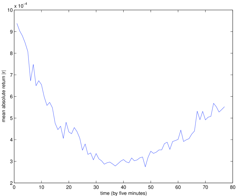
Figure 1: Average absolute return, as a function of time within a trading day. The U-shape characterizes the so-called lunch effect.

For the intra-day Nasdaq data, there are two caveats that must be addressed. First, in order to remove the effect of overnight price jumps, we have determined the returns separately for each of 289 days contained in the Nasdaq data and have taken the union of all these 289 return data sets to obtain a global return data set. Second, the volatility of intra-day data are known to exhibit a U-shape, also called “lunch-effect”, that is, an abnormally high volatility at the begining and the end of the trading day compared with a low volatility at the approximate time of lunch. Such effect is present in our data, as depicted on figure 1, where the average absolute returns are shown as a function of the time within a trading day. It is desirable to correct the data from this systematic effect. This has been performed by renormalizing the 5 minutes-returns at a given moment of the trading day by the corresponding average absolute return at the same moment. We shall refer to this time series as the corrected Nasdaq returns in contrast with the raw (incorrect) Nasdaq returns and we shall examine both data sets for comparison.

The Dow Jones daily returns also exhibit some non-stationarity. Indeed, one can observe a clear excess volatility roughly covering the time of the bubble ending in the October 1929 crash following by the Great Depression. To investigate the influence of such non-stationarity, time interval, the statistical study exposed below has been performed twice: first with the entire sample, and after having removed the period from 1927 to 1936 from the sample. The results are somewhat different, but on the whole, the conclusions about the nature of the tail are the same. Thus, only the results concerning the whole sample will be detailed in the paper.

Although the distributions of positive and negative returns are known to be very similar [JR01, for instance], we have chosen to treat them separately. For the Dow Jones, this gives us $14949$ positive and $13464$ negative data points while, for the Nasdaq, we have $11241$ positive and $10751$ negative data points.

Table 1 summarizes the main statistical properties of these two time series (both for the raw and for the corrected Nasdaq returns) in terms of the average returns, their standard deviations, the skewness and the excess kurtosis for four time scales of five minutes, an hour, one day and one month. The Dow Jones exhibits a significantly negative skewness, which can be ascribed to the impact of the market crashes. The raw Nasdaq returns are significantly positively skewed while the returns corrected for the “lunch effect” are negatively skewed, showing that the lunch effect plays an important role in the shaping of the distribution of the intra-day returns. Note also the important decrease of the kurtosis after correction of the Nasdaq returns for lunch effect, confirming the strong impact of the lunch effect. In all cases, the excess-kurtosis are high and remains significant even after a time aggregation of one month. The Jarque-Bera’s test [Cromwell], a joint statistic using skewness and kurtosis coefficients, is used to reject the normality assumption for these time series.

2.2 Existence of time dependence

It is well-known that financial time series exhibit complex dependence structures like heteroscedasticity or non-linearities. These properties are clearly observed in our two times series. For instance, we have estimated the statistical characteristic $V$ (for positive random variables) called coefficient of variation

$$V=\frac{{\rm Std}(X)}{{\rm E}(X)}~{},$$ (1)

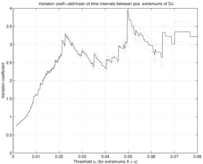
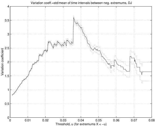
Figure 2: Coefficient of variation $V$ for the Dow Jones daily returns. An increase of $V$ characterizes the increase of “clustering”.

which is often used as a testing statistic of the randomness property of a time series. It can be applied to a sequence of points (or, intervals generated by these points on the line). If these points are “absolutely random,” that is, generated by a Poissonian flow, then the intervals between them are distributed according to an exponential distribution for which $V=1$. If $V<<1$, the process is close to a periodic oscillation. Values $V>>1$ are associated with a clustering phenomenon. We estimated $V=V(u)$ for extrema $X>u$ and $X<-u$ as function of threshold $u$ (both for positive and for negative extrema). The results are shown in figure 2 for the Dow Jones daily returns. As the results are essentially the same for the Nasdaq, we do not show them. Figure 2 shows that, in the main range $|X|<0.02$, containing $\sim 95{\%}$ of the sample, $V$ increases with $u$, indicating that the “clustering” property becomes stronger as the threshold $u$ increases. The coefficient of variation has also been estimated for the Dow Jones when the time interval from 1927 to 1936 is removed. Its maximum value decreases by one, but it still significantly increases with the threshold $u$.

We have then applied several formal statistical tests of independence. We have first performed the Lagrange multiplier test proposed by Engle84 which leads to the $T\cdot R^{2}$ test statistic, where $T$ denotes the sample size and $R^{2}$ is the determination coefficient of the regression of the squared centered returns $x_{t}$ on a constant and on $q$ of their lags $x_{t-1},x_{t-2},\cdots,x_{t-q}$. Under the null hypothesis of homoscedastic time series, $T\cdot R^{2}$ follows a $\chi^{2}$-statistic with $q$ degrees of freedom. The test has been performed up to $q=10$ and, in every case, the null hypothesis is strongly rejected, at any usual significance level. Thus, the time series are heteroskedastic and exhibit volatility clustering. We have also performed a BDS test [BDS87] which allows us to detect not only volatility clustering, like in the previous test, but also departure from iid-ness due to non-linearities. Again, we strongly rejects the null-hypothesis of iid data, at any usual significance level, confirming the Lagrange multiplier test.

3 Can long memory processes lead to misleading measures of extreme properties?

Since the descriptive statistics given in the previous section have clearly shown the existence of a significant temporal dependence structure, it is important to consider the possibility that it can lead to erroneous conclusions on the estimated parameters as previously shown by KP97 for integrated GARCH processes. We first briefly recall the standard procedures used to investigate extremal properties, stressing the problems and drawbacks arising from the existence of temporal dependence. We then perform a numerical simulation to study the behavior of the estimators in presence of dependence. We put particular emphasis on the possible appearance of significant biases due to dependence in the data set. Finally, we present the results on the extremal properties of our two DJ and ND data sets in the light of the bootstrap results.

3.1 Some theoretical results

Two limit theorems allow one to study the extremal properties and to determine the maximum domain of attraction (MDA) of a distribution function in two forms.

First, consider a sample of $N$ iid realizations $X_{1},X_{2},\cdots,X_{N}$. Let $X^{\wedge}$ denotes the maximum of this sample. Then, the Gnedenko theorem states that, if, after an adequate centering and normalization, the distribution of $X^{\wedge}$ converges to a non-degenerate distribution as $N$ goes to infinity, this limit distribution is then necessarily the Generalized Extreme Value (GEV) distribution defined by

$$H_{\xi}(x)=\exp\left[-(1+\xi\cdot x)^{-1/\xi}\right]~{}.$$ (2)

When $\xi=0$, $H_{\xi}(x)$ should be understood as

$$H_{\xi=0}(x)=\exp[-\exp(-x)].$$ (3)

Thus, for $N$ large enough

$$\Pr\left\{X^{\wedge}<x\right\}=H_{\xi}\left(\frac{x-\mu}{\psi}\right),$$ (4)

for some value of the centering parameter $\mu$, scale factor $\psi$ and tail index $\xi$. It should be noted that the existence of non-degenerate limit distribution of properly centered and normalized $X^{\wedge}$ is a rather strong limitation. There are a lot of distribution functions that do not satisfy this limitation, e.g., infinitely alternating functions between a power-like and an exponential behavior.

The second limit theorem is called after Gnedenko-Pickands-Balkema-de Haan (GPBH) and its formulation is as follows. In order to state the GPBH theorem, we define the right endpoint $x_{F}$ of a distribution function $F(x)$ as $x_{F}={\rm sup}\{x:F(x)<1\}$. Let us call the function

$$\Pr\{X-u\geq x~{}|~{}X>u\}\equiv{\bar{F}}_{u}(x)$$ (5)

the excess distribution function (DF). Then, this DF ${\bar{F}}_{u}(x)$ belongs to the Maximum Domain of Attraction of $H_{\xi}(x)$ defined by eq.(2) if and only if there exists a positive scale-function $s(u)$, depending on the threshold $u$, such that

$$\lim_{u\to x_{F}}~{}~{}\sup_{0\leq x\leq x_{F}-u}|{\bar{F}}_{u}(x)-{\bar{G}}(x~{}|~{}\xi,s(u))|=0~{},$$ (6)

where

$$G(x~{}|~{}\xi,s)=1+\ln H_{\xi}\left(\frac{x}{s}\right)=1-\left(1+\xi\cdot\frac{x}{s}\right)^{-1/\xi}~{}.$$ (7)

By taking the limit $\xi\to 0$, expression (7) leads to the exponential distribution. The support of the distribution function (7) is defined as follows:

$$\begin{cases}0\leqslant x<\infty,&\text{ if $\xi\geqslant 0$}\\ 0\leqslant x\leqslant-d/\xi,&\text{ if $\xi<0$}.\end{cases}$$ (8)

Thus, the Generalized Pareto Distribution has a finite support for $\xi<0$.

The form parameter $\xi$ is of paramount importance for the form of the limiting distribution. Its sign determines three possible limiting forms of the distribution of maxima: If $\xi>0$, then the limit distribution is the Fréchet power-like distribution; If $\xi=0$, then the limit distribution is the Gumbel (double-exponential) distribution; If $\xi<0$, then the limit distribution has a support bounded from above. All these three distributions are united in eq.(2) by this parameterization. The determination of the parameter $\xi$ is the central problem of extreme value analysis. Indeed, it allows one to determine the maximum domain of attraction of the underling distribution. When $\xi>0$, the underlying distribution belongs to the Fréchet maximum domain of attraction and is regularly varying (power-like tail). When $\xi=0$, it belongs to the Gumbel Maximum Domain of Attraction and is rapidly varying (exponential tail), while if $\xi<0$ it belongs to the Weibull Maximum Domain of Attraction and has a finite right endpoint.

3.2 Examples of slow convergence to limit GEV and GPD distributions

There exist two ways of estimating $\xi$. First, if there is a sample of maxima (taken from sub-samples of sufficiently large size), then one can fit to this sample the GEV distribution, thus estimating the parameters by Maximum Likelihood method. Alternatively, one can prefer the distribution of exceedances over a large threshold given by the GPD (7), whose tail index can be estimated with Pickands’ estimator or by Maximum Likelihood, as previously. Hill’s estimator cannot be used since it assumes $\xi>0$, while the essence of extreme value analysis is, as we said, to test for the class of limit distributions without excluding any possibility, and not only to determine the quantitative value of an exponent. Each of these methods has its advantages and drawbacks, especially when one has to study dependent data, as we show below.

Given a sample of size $N$, one considers the $q$-maxima drawn from $q$ sub-samples of size $p$ (such that $p\cdot q=N$) to estimate the parameters $(\mu,\psi,\xi)$ in (4) by Maximum Likelihood. This procedure yields consistent and asymptotically Gaussian estimators, provided that $\xi>-1/2$ [Smith85]. The properties of the estimators still hold approximately for dependent data, provided that the interdependence of data is weak. However, it is difficult to choose an optimal value of $q$ of the sub-samples. It depends both on the size $N$ of the entire sample and on the underlying distribution: the maxima drawn from an Exponential distribution are known to converge very quickly to Gumbel’s distribution [HW79], while for the Gaussian law, convergence is particularly slow [Hall79].

The second possibility is to estimate the parameter $\xi$ from the distribution of exceedances (the GPD). For this, one can use either the Maximum Likelihood estimator or Pickands’ estimator. Maximum Likelihood estimators are well-known to be the most efficient ones (at least for $\xi>-1/2$ and for independent data) but, in this particular case, Pickands’ estimator works reasonably well. Given an ordered sample $x_{1}\leq x_{2}\leq\cdots x_{N}$ of size $N$, Pickands’ estimator is given by

$$\hat{\xi}_{k,N}=\frac{1}{\ln 2}\ln\frac{x_{k}-x_{2k}}{x_{2k}-x_{4k}}~{}.$$ (9)

For independent and identically distributed data, this estimator is consistent provided that $k$ is chosen so that $k\rightarrow\infty$ and $k/N\rightarrow 0$ as $N\rightarrow\infty$. Moreover, $\hat{\xi}_{k,N}$ is asymptotically normal with variance

$$\sigma(\hat{\xi}_{k,N})^{2}\cdot k=\frac{\xi^{2}(2^{2\xi+1}+1)}{(2(2^{\xi}-1)\ln 2)^{2}}~{}.$$ (10)

In the presence of dependence between data, one can expect an increase of the standard deviation, as reported by KP97. For time dependence of the GARCH class, KP97 have indeed demonstrated a significant increase of the standard deviation of the tail index estimator, such as Hill’s estimator, by a factor more than seven with respect to their asymptotic properties for iid samples. This leads to very inaccurate index estimates for time series with this kind of temporal dependence.

Another problem lies in the determination of the optimal threshold $u$ of the GPD, which is in fact related to the optimal determination of the sub-samples size $q$ in the case of the estimation of the parameters of the distribution of maximum.

In sum, none of these methods seem really satisfying and each one presents severe drawbacks. The estimation of the parameters of the GEV distribution and of the GPD may be less sensitive to the dependence of the data, but this property is only asymptotic, thus a bootstrap investigation is required to be able to compare the real power of each estimation method for samples of moderate size.

As a first simple example illustrating the possibly very slow convergence to the limit distributions of extreme value theory mentioned above, let us consider a simulated sample of iid Weibull random variables (we thus fulfill the most basic assumption of extreme values theory, i.e, iid-ness). We take two values for the exponent of the Weibull distribution: $c=0.7$ and $c=0.3$, with $d=1$ (scale parameter). An estimation of $\xi$ by the distribution of the GPD of exceedance should give estimated values of $\xi$ close to zero in the limit of large $N$. In order to use the GPD, we have taken the conditional Weibull distribution under condition $X>U_{k},k=1...15$, where the thresholds $U_{k}$ are chosen as: $U_{1}=0.1;~{}U_{2}=0.3;~{}U_{3}=1;~{}U_{4}=3;~{}U_{5}=10;~{}U_{6}=30;~{}U_{7}=100;~{}U_{8}=300;~{}U_{9}=1000;~{}U_{10}=3000;~{}U_{11}=10^{4};~{}U_{12}=3\cdot 10^{4};~{}U_{13}=10^{5};~{}U_{14}=3\cdot 10^{5}$ and $U_{15}=10^{6}$.

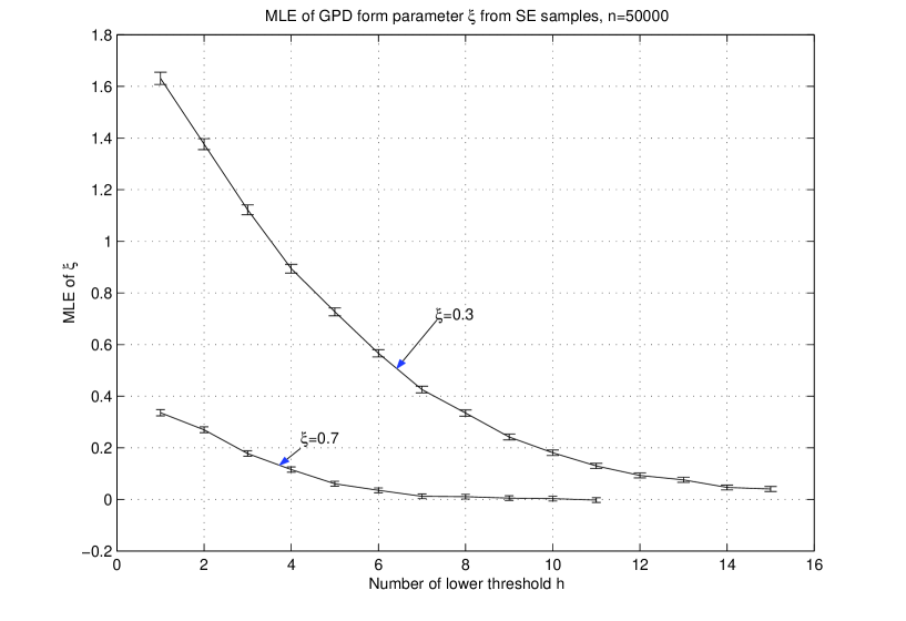
Figure 3: Maximum Likelihood estimates of the GPD form parameter for Stretched-Exponentail samples of size 50,000.

For each simulation, the size of the sample above the considered threshold $U_{k}$ is chosen equal to $50,000$ in order to get small standard deviations. The Maximum-Likelihood estimates of the GPD form parameter $\xi$ are shown in figure 3. For $c=0.7$, the threshold $U_{7}$ gives an estimate $\xi=0.0123$ with standard deviation equal to $0.0045$, i.e., the estimate for $\xi$ differs significantly from zero (recall that $\xi=0$ is the correct theoretical limit value). This occurs notwithstanding the huge size of the implied data set; indeed, the probability $\Pr{X>U_{7}}$ for $c=0.7$ is about $10^{-9}$, so that in order to obtain a data set of conditional samples from an unconditional data set of the size studied here ($50,000$ realizations above $U_{7}$), the size of such unconditional sample should be approximately $10^{9}$ times larger than the number of “peaks over threshold”, i.e., it is practically impossible to have such a sample. For $c=0.3$, the convergence to the theoretical value zero is even slower. Indeed, even the largest financial datasets for a single asset, drawn from high frequency data, are no larger than or of the order of one million points. The situation does not change even for data sets one or two orders of magnitudes larger as considered in [GMAS98, GMAS98_2, Plerouetal99], obtained by aggregating thousands of stocks. Thus, although the GPD form parameter should be zero theoretically in the limit of large sample for the Weibull distribution, this limit cannot be reached for any available sample sizes.

This is a clear illustration that a rapidly varying distribution, like the Weibull distribution with exponent smaller than one, i.e., a Stretched-Exponential distribution, can be mistaken for a Pareto or any other regularly varying distribution for any practical applications.

3.3 Generation of a long memory process with a well-defined stationary distribution

In order to study the performance of the various estimators of the tail index $\xi$ and the influence of interdependence of sample values, we have generated several samples with distinct properties. The first three samples are made of iid realizations drawn respectively from an asymptotic power-law distribution with tail index $b=3$ and from a Stretched-Exponential distribution with exponent $c=0.3$ and $c=0.7$. The other samples contain realizations exhibiting different degrees of time dependence with the same three distributions as for the first three samples: a regularly varying distribution with tail index $b=3$ and a Stretched-Exponential distribution with exponent $c=0.3$ and $c=0.7$. Thus, the three first samples are the iid counterparts of the later ones. The sample with regularly varying iid distributions converges to the Fréchet’s maximum domain of attraction with $\xi=1/3=0.33$, while the iid Stretched-Exponential distribution converges to Gumbel’s maximum domain of attraction with $\xi=0$. We now study how well can one distinguish between these two distributions belonging to two different maximum domains of attraction.

For the stochastic processes with temporal dependence, we use a simple stochastic volatility model. First, we construct a Markovian Gaussian process $\{X_{t}\}_{t\geq 1}$ whose correlation function is

$$C(t)=a^{|t|},\quad a<1.$$ (11)

Varying $a$ allows us to change the strength of the time dependence, characterized by the correlation length $\tau=-\frac{1}{\ln a}$. When $a=0$, the iid case is retrieved. In the following, we have chosen $a=0.95$ and $0.99$, which correspond to correlation lengths of about 20 and 100 lags respectively. For simplicity, we will refer to the first case as the “short-memory” process, while the second one will be called “long-memory” process. This denomination is only for convenience and does not refer to the conventional distinction between processes with short and long range memory [Beran94].

The next step consists in building the process $\{U_{t}\}_{t\geq 1}$, defined by

$$U_{t}=\Phi(X_{t})~{},$$ (12)

where $\Phi(\cdot)$ is the Gaussian distribution function. The process $\{U_{t}\}_{t\geq 1}$ exhibits also a dependence qualitatively similar to that of the process $\{X_{t}\}_{t\geq 1}$. The precise nature of the temporal dependence of the process $\{U_{t}\}_{t\geq 1}$ is revealed differently by different tools Indeed, if one quantifies dependence by copulas, then the process $\{U_{t}\}_{t\geq 1}$ has the same dependence as $\{X_{t}\}_{t\geq 1}$ because copulas are invariant under a strickly increasing change of variables. Let us recall that a copula is the mathematical embodiment of the dependence structure between different random variables [Joe97, Nelsen98]. The process $\{U_{t}\}_{t\geq 1}$ thus possesses a Gaussian copula dependence structure with long memory and uniform marginals. In contrast, if one quantifies the dependence by the correlation coefficient or the correlation ratio or other reasonable standard measures of dependence, the monotonous change of variable (12) is no more innocuous as the correlation may become as small as one wants under an suitable choice of a strickly increasing transformation (see for instance [Malconcept] for a detailed discussion of the effect of conditioning on correlation measures). However, in the present case, we can calculate exactly the correlation function of the process $\{U_{t}\}_{t\geq 1}$, which is nothing but the rank (or Spearman) correlation function of the process $\{X_{t}\}_{t\geq 1}$, so that

$$C_{U}(t) = \frac{6}{\pi}\arcsin\left(\frac{1}{2}~{}C(t)\right),$$ (13)

$$= \frac{6}{\pi}\arcsin\left(\frac{a^{|t|}}{2}\right),$$ (14)

$$\simeq \frac{3}{\pi}a^{|t|},\quad{\rm as}~{}t\rightarrow\infty.$$ (15)

For our purpose, the important point is to obtain a process with the correct asymptotic distribution tails together with some dependence: this allows us to probe some impact of the dependence on estimators and show that standard statistical estimators may become unreliable.

In the last step, we define the volatility process

$$\sigma_{t}=\sigma_{0}\cdot U_{t}^{-1/b}~{},$$ (16)

which ensures that the stationary distribution of the volatility is a Pareto distribution with tail index $b$. Such a distribution of the volatility is not realistic in the bulk which is found to be approximately a lognormal distribution for not too large volatilities [SSA00], but is in agreement with the hypothesis of an asymptotic regularly varying distribution. A change of variable more complicated than (16) can provide a more realistic behavior of the volatility on the entire range of the distribution but our main goal is not to provide a realistic stochastic volatility model but only to exhibit a stochastic process with time dependence and well-defined prescribed marginals in order to test the influence of the dependence structure.

The return process is then given by

$$r_{t}=\sigma_{t}\cdot\epsilon_{t}~{},$$ (17)

where the $\epsilon_{t}$ are Gaussian random variables independent from $\sigma_{t}$. The construction (17) ensures the de-correlation of the returns at every time lag. The stationary distribution of $r_{t}$ admits the density

$$p(r)=\frac{2^{\frac{b}{2}-1}}{\sqrt{\pi}}\cdot\Gamma\left(\frac{b+1}{2},\frac{r^{2}}{2\sigma_{0}^{2}}\right)\frac{b\cdot\sigma_{0}^{b}}{|r|^{b+1}}~{},$$ (18)

which is regularly varying at infinity since $\Gamma\left(\frac{b+1}{2},\frac{r^{2}}{2\cdot\sigma_{0}^{2}}\right)$ goes to $\Gamma\left(\frac{b+1}{2}\right)$. This completes the construction and characterization of our long memory process with regularly varying stationary distribution.

In order to obtain a process with Stretched-Exponential distribution with long range dependence, we apply to $\{r_{t}\}_{t\geq 1}$ the following increasing mapping $G:r\rightarrow y$

$$G(r)=\begin{cases}(x_{0}+\ln\frac{r}{r_{0}})^{1/c}&r>r_{0}\\ {\rm sgn}(r)\cdot|r|^{1/c}&|r|\leq r_{0}\\ -(r_{0}+\ln|r/r_{0}|)^{1/c}&r<-r_{0}~{}.\end{cases}$$ (19)

This transformation gives a stretched exponential of index $c$ for all values of the return larger than the scale factor $r_{0}$. This derives from the fact that the process $\{r_{t}\}_{t\geq 1}$ admits a regularly varying distribution function, characterized by $\bar{F}_{r}(r)=1-F_{r}(r)={\cal L}(r)|r|^{-b}$, for some slowly varying function ${\cal L}$. As a consequence, the stationary distribution of $\{Y_{t}\}_{t\geq 1}$ is given by

$$\bar{F}_{Y}(y) = {\cal L}\left(r_{0}e^{-x_{0}}\exp\left(y^{c}\right)\right)\frac{e^{br_{0}}}{x_{0}^{b}}\cdot e^{-b|y|^{c}},\quad\forall|y|>r_{0},$$ (20)

$$= {\cal L}^{\prime}(y)\cdot e^{-b|y|^{c}},\quad\text{${\cal L}^{\prime}$ is slowly varying at infinity},$$ (21)

which is a Stretched-Exponential distribution.

To summarize, starting with a Markovian Gaussian process, we have defined a stochastic process characterized by a stationary distribution function of our choice, thanks to the invariance of the temporal dependence structure (the copula) under strictly increasing change of variable. In particular, this approach gives stochastic processes with a regularly varying marginal distribution and with a stretched-exponential distribution. Notwithstanding the difference in their marginals, these two processes possess by construction exactly the same time dependence. This allows us to compare the impact of the same dependence on these two classes of marginals.

3.4 Results of numerical simulations

We have generated $1000$ replications of each process presented in the previous section, i.e., iid Stretched-Exponential, iid Pareto, short and long memory processes with a Pareto distribution and with a Stretched-Exponential distribution. Each sample contains $10,000$ realizations, which is approximately the number of points in each tail of our real samples.

Panel (a) of table 2 presents the mean values and standard deviations of the Maximum Likelihood estimates of $\xi$, using the Generalized Extreme Value distribution and the Generalized Pareto Distribution for the three samples of iid data. To estimate the parameters of the GEV distribution and study the influence of the sub-sample size, we have grouped the data in clusters of size $q=10,20,100$ and $200$. For the analysis in terms of the GPD, we have considered four different large thresholds $u$, corresponding to the quantiles $90\%$, $95\%$, $99\%$ and $99.5\%$. The estimates of $\xi$ obtained from the distribution of maxima are compatible (at the $95\%$ confidence level) with the expected value for the Stretched-Exponential with $c=0.7$ for all cluster sizes and for the Pareto distribution for clusters of size larger than 10. For the Stretched-Exponential with fractional exponent $c=0.3$, we obtain an average value $\xi$ larger than $0.2$ over the four different sizes of sub-samples. Except for the largest cluster, this value is significantly different from the theoretical value $\xi=0.0$. This clearly shows that the distribution of the maximum drawn from a Stretched-Exponential distribution with $c=0.7$ converges very quickly toward the theoretical asymptotic GEV distribution, while for $c=0.3$ the convergence is extremely slow. Such a fast convergence for $c=0.7$ is not surprising since, for this value of the fractional index, the Stretched-Exponential distribution remains close to the Exponential distribution, which is known to converge very quickly to the GEV distribution [HW79]. For $c=0.3$, the Stretched-Exponential distribution behaves, over a wide range, like the power law - as we shall see in the next section - thus it is not surprising to obtain an estimate of $\xi$ which remains significantly positive.

Overall, the results are slightly better for the Maximum Likelihood estimates obtained from the GPD. Indeed, the bias observed for the Stretched-Exponential with $c=0.3$ seems smaller for large quantiles than the smallest biases reached by the GEV method. Thus, it appears that the distribution of exceedance converges faster to its asymptotic distribution than the distribution of maximum. However, while in line with the theoretical values, the standard deviations are found almost always larger than in the previous case, which testifies of the higher variability of this estimator. Thus, for such sample sizes, the GEV and GPD Maximum Likelihood estimates should be handled with care and there results interpreted with caution due to possibly important bias and statistical fluctuations. If a small value of $\xi$ seems to allow one to reliably conclude in favor of a rapidly varying distribution, a positive estimate does not appear informative, and in particular does not allow one to reject the rapidly varying behavior of a distribution.

Panel (b) and (c) of table 2 presents the same results for data with short and long memory, respectively. We note the presence of a significant downward bias (with respect to the iid case) in almost every cases for the GPD estimates: the stronger the dependence, the more important is the bias. At the same time, the empirical values of the standard deviations remain comparable with those obtained in the previous case for iid data. The downward bias can be ascribed to the dependence between data. Indeed, positive dependence yields important clustering of extremes and accumulation of realizations around some values, which – for small samples – could (misleadingly) appear as the consequence of the compactness of the support of the underlying distribution. This rationalizes the negative $\xi$ estimates obtained for the Stretched-Exponential distribution with $c=0.7$. In other words, for finite sample, the dependence prevents the full exploration of the tails and create clusters that mimics a thinner tail (even if the clusters are occurring all at large values since what is important is the range of exploration of the tail in order to control the value of $\xi$).

The situation is different for the GEV estimates which show either an upward or downward bias (with respect to the iid case). Here two effects are competing. On the one hand, the dependence creates a downward bias, as explained above, while, on the other hand, the lack of convergence of the distribution of maxima toward its GEV asymptotic distribution results in an upward bias, as observed on iid data. This last phenomemon is strengthened by the existence of time dependence which leads to decrease the “effective” sample size ( the actual size divided by the correlation length $\lambda=\sum C(t)=(1-a)^{-1}$) and thus slows down the convergence rate toward the asymptotic distribution even more. Interestingly, both the GEV and GPD estimators for the Pareto distribution may be utterly wrong in presence of long range dependence for any cluster sizes.

To summarize, two opposite effects are competing. On the one hand, non-asymptotic effects due to the slow convergence toward the asymptotic GEV or GPD distributions yield an upward or downward bias. This effect seems more pronounced for GEV distributions and becomes more important when the correlation length increases since the “effective” sample size decreases. On the other hand, the presence of dependence in the data induces a downward bias and sometimes an increase of the standard deviation of the estimated values. The qualitative effect can be described as follows: the larger $a$ is, the smaller is the $\xi$-estimate, provided - of course - that the “effective” sample size is kept constant, everything being otherwise taken equal.

These two entangled effects, which sometimes compete and sometimes oppose each other, have also been observed for non-Markovian processes drawn from Gaussian processes with long range correlation. Thus, the existence of an important bias and the increase in the scattering of estimates is a general and genuine progeny of the time dependence. It leads us to the conclusion that the Maximum Likelihood estimators derived from the GEV or GPD distributions are not very efficient for the investigation of the financial data whose sample sizes are moderate and which exhibit complicated serial dependence. The only positive note is that the GPD estimator correctly recovers the range of the index $\xi$ with an uncertainty smaller than $20\%$ for data with a pure Pareto distribution while it is cannot reject the hypothesis that $\xi=0$ when the data is generated with a Stretched-Exponential distribution, albeit with a very large uncertainty, in other words with little power.

Table 3 focuses on the results given by Pickands’ estimator for the tail index of the GPD. For each thresholds $u$, corresponding to the quantiles $90\%$, $95\%$, $99\%$ and $99.5\%$ respectively, the results of our simulations are given for two particular values of $k$ (defined in (9)) corresponding to $N/k=4$, which is the largest admissible value, and $N/k=10$ corresponding to be sufficiently far in the tail of the GPD. Table 3 provides the mean value and the numerically estimated as well as the theoretical (given by (10)) standard deviation of $\hat{\xi}_{k,N}$. Panel (a) gives the result for iid data. The mean values do not exhibit a significant bias for the Pareto distribution and the Stretched-Exponential with $c=0.7$, but are utterly wrong in the case $c=0.3$ since the estimates are comparable with those given for the Pareto distribution. In each case, we note a very good agreement between the empirical and theoretical standard deviations, even for the larger quantiles (and thus the smaller samples). Panels (b-c) present the results for dependent data. The estimated standard deviations remains of the same order as the theoretical ones, contrarily to results reported by KP97 for IGARCH processes. However, like these authors, we find that the bias, either positive or negative, becomes very significant and leads one to misclassify a Stretched-Exponential distribution with $c=0.3$ for a Pareto distribution with $b=3$. Thus, in presence of dependence, Pickands’ estimator is unreliable.

To summarize, the determination of the maximum domain of attraction with usual estimators does not appear to be a very efficient way to study the extreme properties of dependent times series. Almost all the previous studies which have investigated the tail behavior of asset returns distributions have focused on these methods (see the influential works of Longin96 for instance) and may thus have led to spurious results on the determination of the tail behavior. In particular, our simulations show that rapidly varying function may be mistaken for regularly varying functions. Thus, according to our simulations, this casts doubts on the strength of the conclusion of previous works that the distributions of returns are regularly varying as seems to have been the consensus until now and suggests to re-examine the possibility that the distribution of returns may be rapidly varying as suggested by GJ98 or LS99 for instance. We now turn to this question using the framework of GEV and GDP estimators just described.

3.5 GEV and GPD estimators of the Dow Jones and Nasdaq data sets

We have applied the same analysis as in the previous section on the real samples of the Dow Jones and Nasdaq (raw and corrected) returns. In order to estimate the standard deviations of Pickands’ estimator for the GPD derived from the upper quantiles of these distributions, and of ML-estimators for the distribution of maximum and for the GPD, we have randomly generated one thousand sub-samples, each sub-sample being constituted of ten thousand data points in the positive or negative parts of the samples respectively (with replacement). It should be noted that the ML-estimates themselves were derived from the full samples. The results are given in tables 4 and 5.

These results confirm the confusion about the tail behavior of the returns distributions and it seems impossible to exclude a rapidly varying behavior of their tails. Indeed, even the estimations performed by Maximum Likelihood with the GPD tail index, which have appeared as the least unreliable estimator in our previous tests, does not allow us to clearly reject the hypothesis that the tails of the empirical distributions of returns are rapidly varying, in particular for large quantile values. For the Nasdaq dataset, accounting for the lunch effect does not yield any significant change in the estimations. This observation will be confirmed by the other tests presented in the next sections.

As a last non-parametric attempt to distinguish between a regularly varying tail and a rapidly varying tail of the exponential or Stretched-Exponential families, we study the Mean Excess Function which is one of the known methods that often can help in deciding what parametric family is appropriate for approximation (see for details EKM97). The Mean Excess Function $MEF(u)$ of a random value $X$ (also called “shortfall” when applied to negative returns in the context of financial risk management) is defined as

$$MEF(u)={\rm E}(X-u|X>u)~{}.$$ (22)

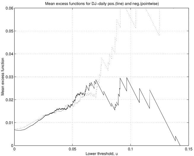
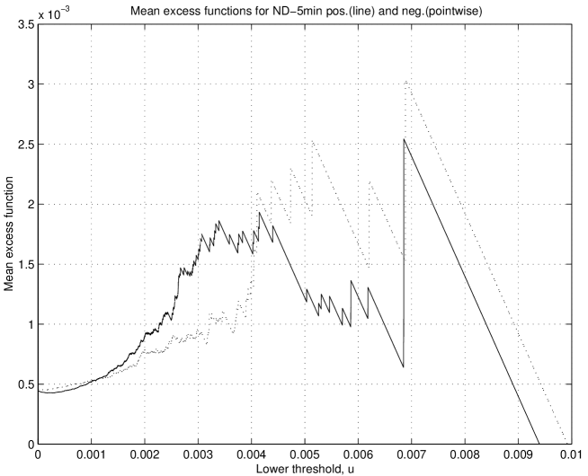
Figure 4: Mean excess functions for the Dow Jones daily returns (upper panel) and the Nasdaq five minutes returns (lower panel). The plain line represents the positive returns and the dotted line the negative ones

The Mean Excess Function $MEF(u)$ is obviously related to the GPD for sufficiently large threshold $u$ and its behavior can be derived in this limit for the three maximum domains of attraction. In addition, more precise results can be given for particular random variables, even in a non-asymptotic regime. Indeed, for an exponential random variable $X$, the $MEF(u)$ is just a constant. For a Pareto random variable, the $MEF(u)$ is a straight increasing line, whereas for the Stretched-Exponential and the Gauss distributions, the $MEF(u)$ is a decreasing function. We evaluated the sample analogues of the $MEF(u)$ [EKM97, p.296] which are shown in figure 4. All attempts to find a constant or a linearly increasing behavior of the $MEF(u)$ on the main central part of the range of returns were ineffective. In the central part of the range of negative returns $(|X|>0.002$; $q\cong 98\%$ for ND data, and $|X|>0.025$ ; $q\cong 96\%$ for DJ data), the $MEF(u)$ behaves like a convex function which exclude both exponential and power (Pareto) distributions. Thus, the $MEF(u)$ tool does not support using any of these two distributions.

An alternative to the Mean Excess function is provided by the Mean Log-Excess function:

$$MLEF(u)={\rm E}(\log(X/u)|X>u).$$ (23)

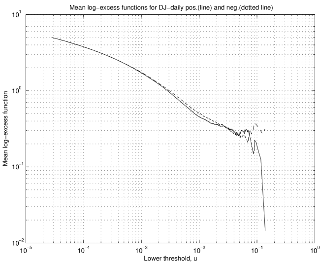
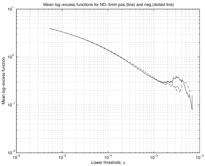
Figure 5: Mean Log-excess functions for the Dow Jones daily returns (upper panel) and the Nasdaq five minutes returns (lower panel). The plain line represents the positive returns and the dotted line the negative ones

$MLEF(u)$ is again related to the GPD (of the variable $\log X$ instead of $X$) for sufficiently large threhold $u$. In particular, when $X$ follows asymtotically a power law, $\log X$ is asymptotically exponentially distributed, so that $MLEF(u)$ goes to a constant equal to $\alpha^{-1}$, where $\alpha$ denotes the tail index of the distribution of $X$. For a Stretched-Exponential variable $X$ with fractional exponent $c$, it turns out that $MLEF(u)$ behaves like a regularly varying function whose tail index equals $-c$. Thus, in a double logarithmic plot, such a behavior is characterized by a decreasing straigth line with slope $-c$. Sample estimates of $MLEF(u)$ are shown in figure 5. On about $90\%$ of the range of the sample, the Mean Log-Excess functions behaves as expected for Stretched-Exponentially distributed variables, while in the tail range (about $10\%$ of the largest values), the results are very confusing, due to the importance of the statistical fluctuations. Such behavior of $MLEF(u)$ in the tails cannot be attributed definitely to a regularly varying or to a Stretched-Exponentially distributed random variable. Therefore, a change of regime cannot be excluded in the extreme tail of the distributions.

In view of the stalemate reached with the above non-parametric approaches and in particular with the standard extreme value estimators, the sequel of this paper is devoted to the investigation of a parametric approach in order to decide which class of extreme value distributions, rapidly versus regularly varying, accounts best for the empirical distributions of returns.

4 Fitting distributions of returns with parametric densities

Since our previous results lead to doubt the validity of the rejection of the hypothesis that the distribution of returns are rapidly varying, we now propose to pit a parametric champion for this class of functions against the Pareto champion of regularly varying functions. To represent the class of rapidly varying functions, we propose the family of Stretched-Exponentials. As discussed in the introduction, the class of stretched exponentials is motivated in part from a theoretical view point by the fact that the large deviations of multiplicative processes are generically distributed with stretched exponential distributions [FrischSor]. Stretched exponential distributions are also parsimonious examples of sub-exponential distributions with fat tails for instance in the sense of the asymptotic probability weight of the maximum compared with the sum of large samples [Feller]. Notwithstanding their fat-tailness, Stretched Exponential distributions have all their moments finite, in contrast with regularly varying distributions for which moments of order equal to or larger than the index $b$ are not defined. This property may provide a substantial advantage to exploit in generalizations of the mean-variance portfolio theory using higher-order moments [R73, FL97, HS99, SSA00, AS01, JM02, MSmm02, for instance ]. Moreover, the existence of all moments is an important property allowing for an efficient estimation of any high-order moment, since it ensures that the estimators are asymptotically Gaussian. In particular, for Stretched-Exponentially distributed random variables, the variance, skewness and kurtosis can be well estimated, contrarily to random variables with regularly varying distribution with tail index in the range $3-5$.

4.1 Definition of two parametric families

4.1.1 A general $3$-parameters family of distributions

We thus consider a general $3$-parameters family of distributions and its particular restrictions corresponding to some fixed value(s) of two (one) parameters. This family is defined by its density function given by:

$$f_{u}(x|b,c,d)=\begin{cases}A(b,c,d,u)~{}x^{-(b+1)}\exp\left[-\left(\frac{x}{d}\right)^{c}\right]&\text{if $x\geqslant u>0$}\\ 0&\text{if $x<u$}.\end{cases}$$ (24)

Here, $b,c,d$ are unknown parameters, $u$ is a known lower threshold that will be varied for the purposes of our analysis and $A(b,c,d,u)$ is a normalizing constant given by the expression:

$$A(b,c,d,u)=\frac{d^{b}~{}c}{\Gamma(-b/c,(u/d)^{c})},$$ (25)

where $\Gamma(a,x)$ denotes the (non-normalized) incomplete Gamma function. The parameter $b$ ranges from minus infinity to infinity while $c$ and $d$ range from zero to infinity. In the particular case where $c=0$, the parameter $b$ also needs to be positive to ensure the normalization of the probability density function (pdf). The interval of definition of this family is the positive semi-axis. Negative log-returns will be studied by taking their absolute values. The family (24) includes several well-known pdf’s often used in different applications. We enumerate them.

1. The Pareto distribution:

   $$F_{u}(x)=1-(u/x)^{b},$$ (26)

   which corresponds to the set of parameters $(b>0,c=0)$ with $A(b,c,d,u)=b\cdot u^{b}$. Several works have attempted to derive or justified the existence of a power tail of the distribution of returns from agent-based models [chalmar], from optimal trading of large funds with sizes distributed according to the Zipf law [gabaixstan] or from stochastic processes [SF02, Biham98, 2002].

2. The Weibull distribution:

   $$F_{u}(x)=1-\exp\left[-\left(\frac{x}{d}\right)^{c}+\left(\frac{u}{d}\right)^{c}\right],$$ (27)

   with parameter set $(b=-c,c>0,d>0)$ and normalization constant $A(b,c,d,u)=\frac{c}{d^{c}}\exp\left[\left(\frac{u}{d}\right)^{c}\right]$. This distribution is said to be a “Stretched-Exponential” distribution when the exponent $c$ is smaller than $1$, namely when the distribution decays more slowly than an exponential distribution.

3. The exponential distribution:

   $$F_{u}(x)=1-\exp\left(-\frac{x}{d}+\frac{u}{d}\right),$$ (28)

   with parameter set $(b=-1,~{}c=1,~{}d>0)$ and normalization constant $A(b,c,d,u)=\frac{1}{d}\exp\left(-\frac{u}{d}\right)$. For sufficiently high quantiles, the exponential behavior can for instance derive, from the hyperbolic model introduced by Eberlein or from a simple model where stock price dynamics is governed by a geometrical (multiplicative) Brownian motion with stochastic variance. Dragu have found an excellent fit of the Dow-Jones index for time lags from 1 to 250 trading days with a model with an asymptotic exponential tail of the distribution of log-returns.

4. The incomplete Gamma distribution:

   $$F_{u}(x)=1-\frac{\Gamma(-b,x/d)}{\Gamma(-b,u/d)}$$ (29)

   with parameter set $(b,~{}c=1,~{}d>0)$ and normalization $A(b,c,d,u)=\frac{d^{b}}{\Gamma(-b,u/d)}$. Such an asymptotic tail behavior can, for instance, be observed for the generalized hyperbolic models, whose description can be found in Prause.

Thus, the Pareto distribution (PD) and exponential distribution (ED) are one-parameter families, whereas the stretched exponential (SE) and the incomplete Gamma distribution (IG) are two-parameter families. The comprehensive distribution (CD) given by equation (24) contains three unknown parameters.

Interesting links between these different models reveal themselves under specific asymptotic conditions. Very interesting for our present study is the behavior of the (SE) model when $c\to 0$ and $u>0$. In this limit, and provided that

$$c\cdot\left(\frac{u}{d}\right)^{c}\rightarrow\beta,\quad\text{as}~{}c\rightarrow 0~{}.$$ (30)

the (SE) model goes to the Pareto model. Indeed, we can write

$$\frac{c}{d^{c}}\cdot x^{c-1}\cdot\exp\left(-\frac{x^{c}-u^{c}}{d^{c}}\right) = c\left(\frac{u}{d}\right)^{c}\cdot\frac{x^{c-1}}{u^{c}}\exp\left[-\left(\frac{u}{d}\right)^{c}\cdot\left(\left(\frac{x}{u}\right)^{c}-1\right)\right]~{},$$ (31)

$$\simeq \beta\cdot x^{-1}\exp\left[-c\left(\frac{u}{d}\right)^{c}\cdot\ln\frac{x}{u}\right],\quad\text{as}~{}c\rightarrow 0$$

$$\simeq \beta\cdot x^{-1}\exp\left[-\beta\cdot\ln\frac{x}{u}\right]~{},$$

$$\simeq \beta\frac{u^{\beta}}{x^{\beta+1}}~{},$$

which is the pdf of the (PD) model with tail index $\beta$. The condition (30) comes naturally from the properties of the maximum-likelihood estimator of the scale parameter $d$ given by equation (52) in Appendix A. It implies that, as $c\to 0$, the characteristic scale $d$ of the (SE) model must also go to zero with $c$ to ensure the convergence of the (SE) model towards the (PD) model.

This shows that the Pareto model can be approximated with any desired accuracy on an arbitrary interval $(u>0,U)$ by the (SE) model with parameters $(c,d)$ satisfying equation (30) where the arrow is replaced by an equality. Although the value $c=0$ does not give strickly speaking a Stretched-Exponential distribution, the limit $c\rightarrow 0$ provides any desired approximation to the Pareto distribution, uniformly on any finite interval $(u,U)$. This deep relationship between the SE and PD models allows us to understand why it can be very difficult to decide, on a statistical basis, which of these models fits the data best.

Another interesting behavior is obtained in the limit $b\to+\infty$, where the Pareto model tends to the Exponential model [BP00]. Indeed, provided that the scale parameter $u$ of the power law is simultaneously scaled as $u^{b}=(b/\alpha)^{b}$, we can write the tail of the cumulative distribution function of the PD as $u^{b}/(u+x)^{b}$ which is indeed of the form $u^{b}/x^{b}$ for large $x$. Then, $u^{b}/(u+x)^{b}=(1+\alpha x/b)^{-b}\to\exp(-\alpha x)$ for $b\to+\infty$. This shows that the Exponential model can be approximated with any desired accuracy on intervals $(u,u+A)$ by the (PD) model with parameters $(\beta,u)$ satisfying $u^{b}=(b/\alpha)^{b}$, for any positive constant A. Although the value $b\to+\infty$ does not give strickly speaking a Exponential distribution, the limit $u\propto b\rightarrow+\infty$ provides any desired approximation to the Exponential distribution, uniformly on any finite interval $(u,u+A)$. This limit is thus less general that the SE $\to$ PD limit since it is valid only asymptotically for $u\rightarrow+\infty$ while $u$ can be finite in the SE $\to$ PD limit.

4.1.2 The log-Weibull family of distributions

Let us also introduce the two-parameter log-Weibull family:

$$1-F(x)=\exp\left[-b\left(\ln(x/u)\right)^{c}\right]~{},~{}~{}~{}~{}{\rm for}~{}~{}x\geq u~{}.$$ (32)

whose density is

$$f_{u}(x|b,c,d)=\begin{cases}\frac{b\cdot c}{x}\left(\ln\frac{x}{u}\right)^{c-1}\exp\left[-b\left(\ln\frac{x}{u}\right)^{c}\right],&\text{if $x\geqslant u>0$}\\ 0,&\text{if $x<u$}.\end{cases}$$ (33)

This family of pdf interpolates smoothly between the Stretched-Exponential and Pareto classes. It recovers the Pareto family for $c=1$, in which case the parameter $b$ is the tail exponent. For $c$ larger than $1$, the tail of the log-Weibull is thinner than any Pareto distribution but heavier than any Stretched-Exponential. In particular, when $c$ equals two, the log-normal distribution is retrieved (above threshold $u$). For $c$ smaller than $1$, the tails of the SLE are even heavier than any Pareto distributions. This range of parameter is probably not useful except maybe to account of “outliers” in the spirit of JS02; this will require a specific investigation.

4.2 Methodology

We start with fitting our two data sets (DJ and ND) by the five distributions enumerated above (24) and (26-29). Our first goal is to show that no single parametric representation among any of the cited pdf’s fits the whole range of the data sets. Recall that we analyze separately positive and negative returns (the later being converted to the positive semi-axis). We shall use in our analysis a movable lower threshold $u$, restricting by this threshold our sample to observations satisfying to $x>u$.

In addition to estimating the parameters involved in each representation (24,26-29) by maximum likelihood for each particular threshold $u$, we need a characterization of the goodness-of-fit. For this, we propose to use a distance between the estimated distribution and the sample distribution. Many distances can be used: mean-squared error, Kullback-Liebler distance, Kolmogorov distance, Sherman distance (as in Longin96) or Anderson-Darling distance, to cite a few. We can also use one of these distances to determine the parameters of each pdf according to the criterion of minimizing the distance between the estimated distribution and the sample distribution. The chosen distance is thus useful both for characterizing and for estimating the parametric pdf. In the later case, once an estimation of the parameters of particular distribution family has been obtained according to the selected distance, we need to quantify the statistical significance of the fit. This requires to derive the statistics associated with the chosen distance. These statistics are known for most of the distances cited above, in the limit of large sample.

We have chosen the Anderson-Darling distance to derive our estimated parameters and perform our tests of goodness of fit. The Anderson-Darling distance between a theoretical distribution function $F(x)$ and its empirical analog $F_{N}(x)$, estimated from a sample of $N$ realizations, is evaluated as follows:

$${\rm ADS} = N\cdot\int\frac{[F_{N}(x)-F(x)]^{2}}{F(x)(1-F(x))}~{}dF(x)$$ (34)

$$= -N-2\sum\limits_{1}^{N}{\{w_{k}\log(F(y_{k}))+(1-w_{k})\log(1-F(y_{k}))\}},$$ (35)

where $w_{k}=2k/(2N+1)$, $k=1\ldots N$ and $y_{1}\leqslant\ldots\leqslant y_{N}$ is its ordered sample. If the sample is drawn from a population with distribution function $F(x)$, the Anderson-Darling statistics (ADS) has a standard AD-distribution free of the theoretical df F(x) [AD52], similarly to the $\chi^{2}$ for the $\chi^{2}$-statistic, or the Kolmogorov distribution for the Kolmogorov statistic. It should be noted that the ADS weights the squared difference in eq.(34) by $1/F(x)(1-F(x))$ which is nothing but the inverse of the variance of the difference in square brackets. The AD distance thus emphasizes more the tails of the distribution than, say, the Kolmogorov distance which is determined by the maximum absolute deviation of $F_{n}(x)$ from $F(x)$ or the mean-squared error, which is mostly controlled by the middle of range of the distribution. Since we have to insert the estimated parameters into the ADS, this statistic does not obey any more the standard AD-distribution: the ADS decreases because the use of the fitting parameters ensures a better fit to the sample distribution. However, we can still use the standard quantiles of the AD-distribution as upper boundaries of the ADS. If the observed ADS is larger than the standard quantile with a high significance level $(1-\varepsilon)$, we can then conclude that the null hypothesis $F(x)$ is rejected with significance level larger than $(1-\varepsilon)$. If we wish to estimate the real significance level of the ADS in the case where it does not exceed the standard quantile of a high significance level, we are forced to use some other method of estimation of the significance level of the ADS, such as the bootstrap method.

In the following, the estimates minimizing the Anderson-Darling distance will be refered to as AD-estimates. The maximum likelihood estimates (ML-estimates) are asymptotically more efficient than AD-estimates for independent data and under the condition that the null hypothesis (given by one of the four distributions (26-29), for instance) corresponds to the true data generating model. When this is not the case, the AD-estimates provide a better practical tool for approximating sample distributions compared with the ML-estimates.

We have determined the AD-estimates for $18$ standard significance levels $q_{1}\ldots q_{18}$ given in table 6. The corresponding sample quantiles corresponding to these significance levels or thresholds $u_{1}\ldots u_{18}$ for our samples are also shown in table 6. Despite the fact that thresholds $u_{k}$ vary from sample to sample, they always corresponded to the same fixed set of significance levels $q_{k}$ throughout the paper and allows us to compare the goodness-of-fit for samples of different sizes.

4.3 Empirical results

The Anderson-Darling statistics (ADS) for six parametric distributions (Weibull or Stretched-Exponential, Generalized Pareto, Gamma, Exponential, Pareto and Log-Weibull) are shown in table 7 for two quantile ranges, the first top half of the table corresponding to the $90\%$ lowest thresholds while the second bottom half corresponds to the $10\%$ highest ones. For the lowest thresholds, the ADS rejects all distributions, except the Stretched-Exponential for the Nasdaq. Thus, none of the considered distributions is really adequate to model the data over such large ranges. For the $10\%$ highest quantiles, only the exponential model is rejected at the $95\%$ confidence level. The Log-Weibull and the Stretched-Exponential distributions are the best, just above the Pareto distribution and the Incomplete Gamma that cannot be rejected. We now present an analysis of each case in more details.

4.3.1 Pareto distribution

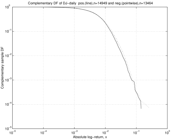
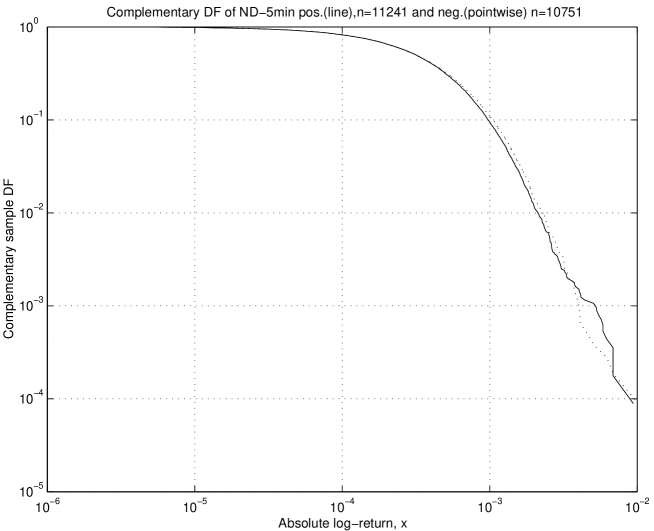
Figure 6: Cumulative sample distributions for the Dow Jones (a) and for the Nasdaq (b) data sets.

Figure 6a shows the cumulative sample distribution function $1-F(x)$ for the Dow Jones Industrial Average index, and in figure 6b the cumulative sample distribution function for the Nasdaq Composite index. The mismatch between the Pareto distribution and the data can be seen with the naked eye: if samples were taken from a Pareto population, the graph in double log-scale should be a straight line. Even in the tails, this is doubtful. To formalize this impression, we calculate the Hill and AD estimators for each threshold $u$. Denoting $y_{1}\geqslant\ldots\geqslant y_{n_{u}}$ the ordered sub-sample of values exceeding $u$ where $N_{u}$ is the size of this sub-sample, the Hill maximum likelihood estimate of parameter $b$ is [Hill75]

$$\hat{b}_{u}=\left[\frac{1}{N_{u}}~{}\sum\limits_{1}^{N_{u}}{\log(y_{k}/u)}\right]^{-1}~{}.$$ (36)

The standard deviations of $\hat{b}_{u}$ can be estimated as

$${\rm Std}(\hat{b}_{u})=\hat{b}_{u}/\sqrt{N_{u}},$$ (37)

under the assumption of iid data, but very severely underestimate the true standard deviation when samples exhibit dependence, as reported by KP97.

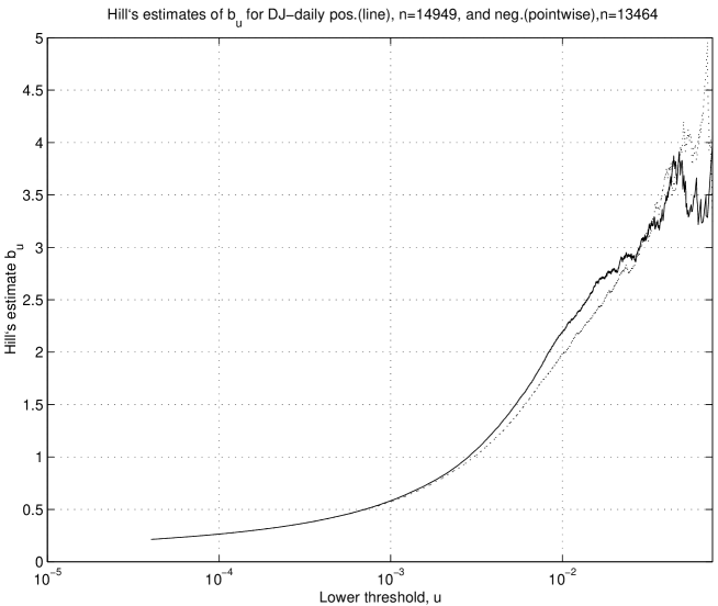
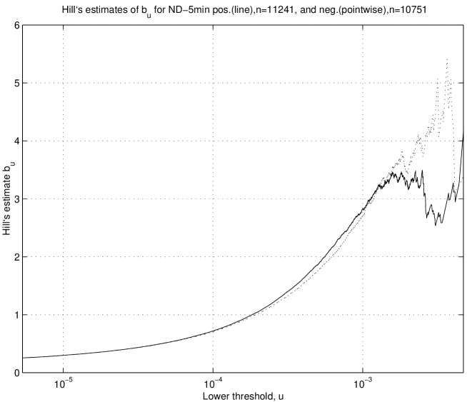
Figure 7: Hill estimates $\hat{b}_{u}$ as a function of the threshold $u$ for the Dow Jones (a) and for the Nasdaq (b).

Figure 7a and 7b shows the Hill estimates $\hat{b}_{u}$ as a function of $u$ for the Dow Jones and for the Nasdaq. Instead of an approximately constant exponent (as would be the case for true Pareto samples), the tail index estimator increases until $u\cong 0.04$, beyond which it seems to slow its growth and oscillates around a value $\approx 3-4$ up to the threshold $u\cong.08$. It should be noted that the interval $[0,0.04]$ contains $99.12\%$ of the sample whereas the interval $[0.04,0.08]$ contains only $0.64\%$ of the sample. The behavior of $\hat{b}_{u}$ for the ND shown in figure 7b is similar: Hill’s estimate $\hat{b}_{u}$ seems to slow its growth already at $u\cong 0.0013$ corresponding to the $95\%$ quantile. Are these slowdowns of the growth of $\hat{b}_{u}$ genuine signatures of a possible constant well-defined asymptotic value that would qualify a regularly varying function?

As a first answer to this question, table 8 compares the AD-estimates of the tail exponent $b$ with the corresponding maximum likelihood estimates for the 18 intervals $u_{1}\ldots u_{18}$. Both maximum likelihood and Anderson-Darling estimates of $b$ steadily increase with the threshold $u$ (except for the highest quantiles of the positive tail of the Nasdaq). The corresponding figures for positive and negative returns are very close to each other and almost never significantly different at the usual $95\%$ confidence level. Some slight non-monotonicity of the increase for the highest thresholds can be explained by small sample sizes. One can observe that both MLE and ADS estimates continue increasing as the interval of estimation is contracting to the extreme values. It seems that their growth potential has not been exhausted even for the largest quantile $u_{18}$, except for the positive tail of the Nasdaq sample. This statement might not be very strong as the standard deviations of the tail index estimators also grow when exploring the largest quantiles. However, the non-exhausted growth is observed for three samples out of the four tails. Moreover, this effect is seen for several threshold values while random fluctuations would distort the $b$-curve in a random manner rather than according to the increasing trend observed in three out of four tails.

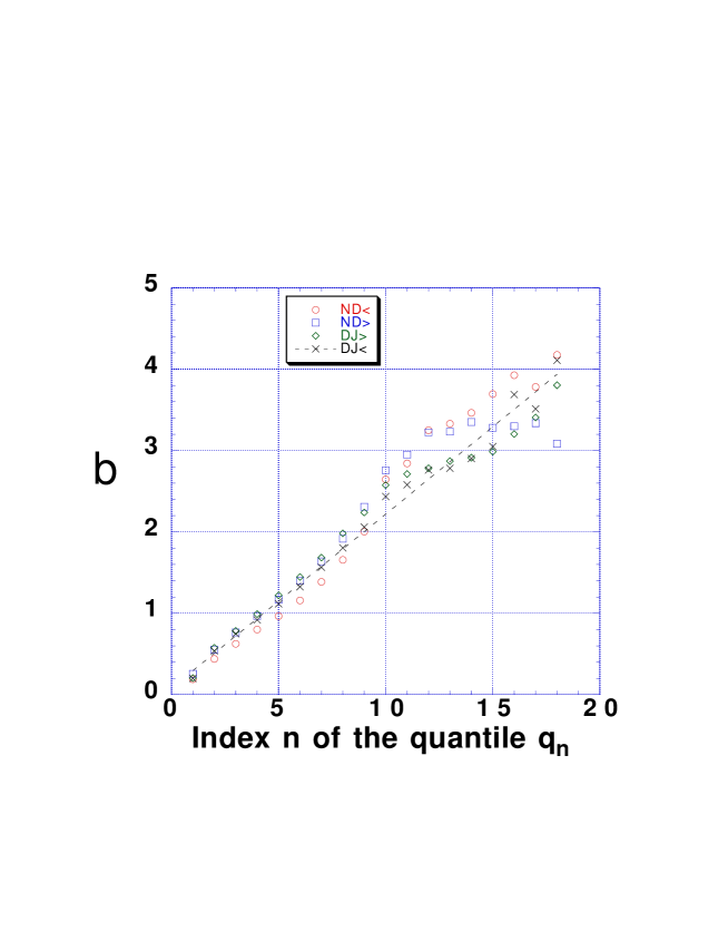
Figure 8: Hill estimator $\hat{b}_{u}$ for all four data sets (positive and negative branches of the distribution of returns for the DJ and for the ND) as a function of the index $n=1,...,18$ of the $18$ quantiles or standard significance levels $q_{1}\ldots q_{18}$ given in table 6. The dashed line is expression (39) with $1-q_{n}=3.08~{}e^{-0.342n}$ given by (38).

Assuming that the observation, that the sample distribution can be approximated by a Pareto distribution with a growing index $b$, is correct, an important question arises: how far beyond the sample this growth will continue? Judging from table 8, we can think this growth is still not exhausted. Figure 8 suggests a specific form of this growth, by plotting the hill estimator $\hat{b}_{u}$ for all four data sets (positive and negative branches of the distribution of returns for the DJ and for the ND) as a function of the index $n=1,...,18$ of the $18$ quantiles or standard significance levels $q_{1}\ldots q_{18}$ given in table 6. Similar results are obtained with the AD estimates. Apart from the positive branch of the ND data set, all other three branches suggest a continuous growth of the Hill estimator $\hat{b}_{u}$ as a function of $n=1,...,18$. Since the quantiles $q_{1}\ldots q_{18}$ given in table 6 have been chosen to converge to $1$ approximately exponentially as

$$1-q_{n}=3.08~{}e^{-0.342n}~{},$$ (38)

the linear fit of $\hat{b}_{u}$ as a function of $n$ shown as the dashed line in figure 8 corresponds to

$$\hat{b}_{u}(q_{n})=0.08+0.626\ln\frac{3.08}{1-q_{n}}~{}.$$ (39)

Expression (39) suggests an unbound logarithmic growth of $\hat{b}_{u}$ as the quantile approaches $1$. For instance, for a quantile $1-q=0.1\%$, expression (39) predicts $\hat{b}_{u}(1-q=10^{-3})=5.1$. For a quantile $1-q=0.01\%$, expression (39) predicts $\hat{b}_{u}(1-q=10^{-4})=6.5$, and so on. Each time the quantile $1-q$ is divided by a factor $10$, the apparent exponent $\hat{b}_{u}(q)$ is increased by the additive constant $\cong 1.45$: $\hat{b}_{u}((1-q)/10)=\hat{b}_{u}(1-q)+1.45$. This very slow growth uncovered here may be an explanation for the belief and possibly mistaken conclusion that the Hill and other estimators of the tail index tends to a constant for high quantiles. Indeed, it is now clear that the slowdowns of the growth of $\hat{b}_{u}$ seen in figures 7 decorated by large fluctuations due to small size effects is mostly the result of a dilatation of the data expressed in terms of threshold $u$. When recast in the more natural logarithm scale of the quantiles $q_{1}\ldots q_{18}$, this slowdown disappears. Of course, it is impossible to know how long this growth given by (39) may go on as the quantile $q$ tends to $1$. In other words, how can we escape from the sample range when estimating quantiles? How can we estimate the so-called “high quantiles” at the level $q>1-1/T$ where $T$ is the total number of sampled points. EKM97 have summarized the situation in this way: “there is no free lunch when it comes to high quantiles estimation!” It is possible that $\hat{b}_{u}(q)$ will grow without limit as would be the case if the true underlying distribution was rapidly varying. Alternatively, $\hat{b}_{u}(q)$ may saturate to a large value, as predicted for instance by the traditional GARCH model which yields tails indices which can reach $10-20$ [EP01, SP99] or by the recent multifractal random walk (MRW) model which gives an asymptotic tail exponent in the range $20-50$ [Muzyetal, musor]. According to (39), a value $\hat{b}_{u}\approx 20$ (respectively $50$) would be attained for $1-q\approx 10^{-13}$ (respectively $1-q\approx 10^{-34}$)! If one believes in the prediction of the MRW model, the tail of the distribution of returns is regularly varying but this insight is completely useless for all practical purposes due to the astronomically high statistics that would be needed to sample this regime. In this context, we cannot hope to get access to the true nature of the pdf of returns but only strive to define the best effective or apparent most parsimonious and robust model. By comparing distributions of aggregated returns with their corresponding reshuffled counterparts, Viswanathan suggest that the fat tail nature of the returns result mainly from the existence of long-range dependence, in agreement with the construction of GARCH and MRW processes.

4.3.2 Weibull distributions

Let us now fit our data with the Weibull (SE) distribution (27). The Anderson-Darling statistics (ADS) for this case are shown in table 7. The ML-estimates and AD-estimates of the form parameter $c$ are represented in table 9. Table 7 shows that, for the highest quantiles, the ADS for the Stretched-Exponential is the smallest of all ADS, suggesting that the SE is the best model of all. Moreover, for the lowest quantiles, it is the sole model not systematically rejected at the $95\%$ level.

The $c$-estimates are found to decrease when increasing the order $q$ of the threshold $u_{q}$ beyond which the estimations are performed. In addition, the $c$-estimate is identically zero for $u_{18}$. However, this does not automatically imply that the SE model is not the correct model for the data even for these highest quantiles. Indeed, numerical simulations show that, even for synthetic samples drawn from genuine Stretched-Exponential distributions with exponent $c$ smaller than $0.5$ and whose size is comparable with that of our data, in about one case out of three (depending on the exact value of $c$) the estimated value of $c$ is zero. This a priori surprising result comes from condition (56) in appendix A which is not fulfilled with certainty even for samples drawn for SE distributions.

Notwithstanding this cautionary remark, note that the $c$-estimate of the positive tail of the Nasdaq data equal zero for all quantiles higher than $q_{14}=0.97\%$. In fact, in every cases, the estimated $c$ is not significantly different from zero - at the $95\%$ significance level - for quantiles higher than $q_{12}$-$q_{14}$. In addition, table 10 gives the values of the estimated scale parameter $d$, which are found very small - particularly for the Nasdaq - beyond $q_{12}=95\%$. In contrast, the Dow Jones keeps significant scale factors until $q_{16}-q_{17}$.

These evidences taken all together provide a clear indication on the existence of a change of behavior of the true pdf of these four distributions: while the bulks of the distributions seem rather well approximated by a SE model, a fatter tailed distribution than that of the (SE) model is required for the highest quantiles. Actually, the fact that both $c$ and $d$ are extremely small may be interpreted according to the asymptotic correspondence given by (30) and (31) as the existence of a possible power law tail.

4.3.3 Exponential and incomplete Gamma distributions

Let us now fit our data with the exponential distribution (28). The average ADS for this case are shown in table 7. The maximum likelihood- and Anderson-Darling estimates of the scale parameter $d$ are given in table 11. Note that they always decrease as the threshold $u_{q}$ increases. Comparing the mean ADS-values of table 7 with the standard AD quantiles, we can conclude that, on the whole, the exponential distribution (even with moving scale parameter d) does not fit our data: this model is systematically rejected at the $95\%$ confidence level for the lowest and highest quantiles - excepted for the negative tail of the Nasdaq.

Finally, we fit our data by the IG-distribution (29). The mean ADS for this class of functions are shown in table 7. The Maximum likelihood and Anderson Darling estimates of the power index $b$ are represented in table 12. Comparing the mean ADS-values of table 7 with the standard AD quantiles, we can again conclude that, on the whole, the IG-distribution does not fit our data. The model is rejected at the $95\%$ confidence level excepted for the negative tail of the Nasdaq for which it is not rejected marginally (significance level: $94.13\%$). However, for the largest quantiles, this model becomes again relevant since it cannot be rejected at the $95\%$ level.

4.3.4 Log-Weibull distributions

The parameters $b$ and $c$ of the log-Weibull defined by (32) are estimated with both the Maximum Likelihood and Anderson-Darling methods for the $18$ standard significance levels $q_{1}\ldots q_{18}$ given in table 6. The results of these estimations are given in table 13. For both positive and negative tails of the Dow Jones, we find very stable results for all quantiles lower than $q_{10}$: $c=1.09\pm 0.02$ and $b=2.71\pm 0.07$. These results reject the Pareto distribution degeneracy $c=1$ at the $95\%$ confidence level. Only for the quantiles higher than or equal to $q_{16}$, we find an estimated value $c$ compatible with the Pareto distribution. Moreover both for the positive and negative Dow Jones tails, we find that $c\approx 0.92$ and $b\approx 3.6-3.8$, suggesting a possible change of regime or a sensitivity to “outliers” or a lack of robustness due to the small sample size. For the positive Nasdaq tail, the exponent $c$ is found compatible with $c=1$ (the Pareto value), at the $95\%$ significance level, above $q_{11}$ while $b$ remains almost stable at $b\simeq 3.2$. For the negative Nasdaq tail, we find that $c$ decreases almost systematically from $1.1$ for $q_{10}$ to $1$ for $q_{18}$ for both estimators while $b$ regularly increases from about $3.1$ to about $4.2$. The Anderson-Darling distances are not worse but not significantly better than for the SE and this statistics cannot be used to conclude neither in favor of nor against the log-Weibull class.

4.4 Summary

At this stage, two conclusions can be drawn. First, it appears that none of the considered distributions fit the data over the entire range, which is not a surprise. Second, for the highest quantiles, four models seem to be able to represent to data, the Gamma model, the Pareto model, the Stretched-Exponential model and the log-Weibull model. The two last ones have the lowest Anderson-Darling statistics and thus seems to be the most reasonable models among the four models compatible with the data. For all the samples, their Anderson-Darling statistic remain so close to each other for the quantiles higher than $q_{10}$ that the descriptive power of these two models cannot be distinguished.

5 Comparison of the descriptive power of the different families

As we have seen by comparing the Anderson-Darling statistics corresponding to the five parametric families (26-29) and (33), the best models in the sense of minimizing the Anderson-Darling distance are the Stretched-Exponential and the Log-Weibull distributions.

We now compare the four distributions (26-29) with the comprehensive distribution (24) using Wilks’ theorem [Wilks38] of nested hypotheses to check whether or not some of the four distributions are sufficient compared with the comprehensive distribution to describe the data. It will appear that the Pareto and the Stretched-Exponential models are the most parsimonious. We then turn to a direct comparison of the best two parameter models (the SE and log-Weibull models) with the best one parameter model (the Pareto model), which will require an extension of Wilks’ theorem derived in Appendix D that will allow us to directly test the SE model against the Pareto model.

5.1 Comparison between the four parametric families (26-29) and the comprehensive distribution (24)

According to Wilks’ theorem, the doubled generalized log-likelihood ratio $\Lambda$:

$$\Lambda=2~{}\log\frac{\max{\cal L}(CD,X,\Theta)}{\max{\cal L}(z,X,\theta)},$$ (40)

has asymptotically (as the size $N$ of the sample $X$ tends to infinity) the $\chi^{2}$-distribution. Here ${\cal L}$ denotes the likelihood function, $\theta$ and $\Theta$ are parametric spaces corresponding to hypotheses $z$ and $CD$ correspondingly (hypothesis $z$ is one of the four hypotheses (26-29) that are particular cases of the $CD$ under some parameter relations). The statement of the theorem is valid under the condition that the sample $X$ obeys hypothesis $z$ for some particular value of its parameter belonging to the space $\theta$. The number of degrees of freedom of the $\chi^{2}$-distribution equals to the difference of the dimensions of the two spaces $\Theta$ and $\theta$. We have $\dim(\Theta)=3,\dim(\theta)=2$ for the Stretched-Exponential and for the Incomplete Gamma distributions while $\dim(\theta)=1$ for the Pareto and the Exponential distributions. This corresponds to one degree of freedom for the two former cases and two degrees of freedom for the later pdf’s. The maximum of the likelihood in the numerator of (40) is taken over the space $\Theta$, whereas the maximum of the likelihood in the denominator of (40) is taken over the space $\theta$. Since we have always $\theta\subset\Theta$, the likelihood ratio is always larger than $1$, and the log-likelihood ratio is non-negative. If the observed value of $\Lambda$ does not exceed some high-confidence level (say, $99\%$ confidence level) of the $\chi^{2}$, we then reject the hypothesis CD in favor of the hypothesis $z$, considering the space $\Theta$ redundant. Otherwise, we accept the hypothesis CD, considering the space $\theta$ insufficient.

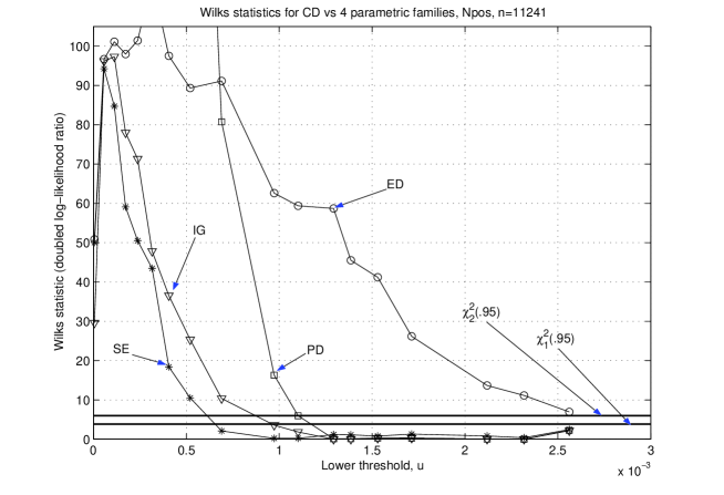
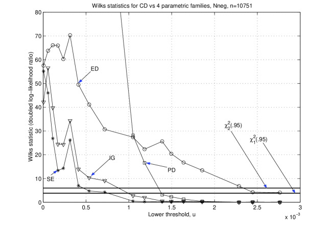
Figure 9: Wilks statistic for the comprehensive distribution versus the four parametric distributions : Pareto (PD), Weibull (SE), Exponential (ED) and Incomplete Gamma (IG) for the Nasdaq five minutes returns. The upper panel refers to the positive returns and lower panel to the negative ones.

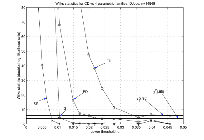
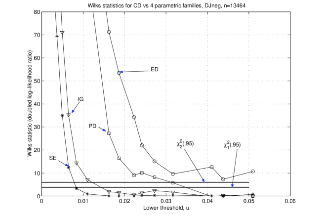
Figure 10: Wilks statistic for the comprehensive distribution versus the four parametric distributions : Pareto (PD), Weibull (SE), Exponential (ED) and Incomplete Gamma (IG) for the Dow Jones daily returns. The upper panel refers to the positive returns and the lower panel to the negative ones.

The doubled log-likelihood ratios (40) are shown in figures 9 for the positive and negative branches of the distribution of returns of the Nasdaq and in figures 10 for the Dow Jones. The $95\%$ $\chi^{2}$ confidence levels for $1$ and $2$ degrees of freedom are given by the horizontal lines.

For the Nasdaq data, figure 9 clearly shows that Exponential distribution is completely insufficient: for all lower thresholds, the Wilks log-likelihood ratio exceeds the $95\%$ $\chi_{1}^{2}$ level $3.84$. The Pareto distribution is insufficient for thresholds $u_{1}-u_{11}$ ($92.5\%$ of the ordered sample) and becomes comparable with the Comprehensive distribution in the tail $u_{12}-u_{18}$ ($7.5\%$ of the tail probability). It is natural that two-parametric families Incomplete Gamma and Stretched-Exponential have higher goodness-of-fit than the one-parametric Exponential and Pareto distributions. The Incomplete Gamma distribution is comparable with the Comprehensive distribution starting with $u_{10}$ ($90\%$), whereas the Stretched-Exponential is somewhat better ($u_{9}$ or $u_{8}$ , i.e., $70\%$). For the tails representing $7.5\%$ of the data, all parametric families except for the Exponential distribution fit the sample distribution with almost the same efficiency. The results obtained for the Dow Jones data shown in figure 10 are similar. The Stretched-Exponential is comparable with the Comprehensive distribution starting with $u_{8}$ ($70\%$). On the whole, one can say that the Stretched-Exponential distribution performs better than the three other parametric families.

We should stress that each log-likelihood ratio represented in figures 9 and 10, so-to say “acts on its own ground,” that is, the corresponding $\chi^{2}$-distribution is valid under the assumption of the validity of each particular hypothesis whose likelihood stands in the numerator of the double log-likelihood (40). It would be desirable to compare all combinations of pairs of hypotheses directly, in addition to comparing each of them with the comprehensive distribution. Unfortunately, the Wilks theorem can not be used in the case of pair-wise comparison because the problem is not more that of comparing nested hypothesis (that is, one hypothesis is a particular case of the comprehensive model). As a consequence, our results on the comparison of the relative merits of each of the four distributions using the generalized log-likelihood ratio should be interpreted with a care, in particular, in a case of contradictory conclusions. Fortunately, the main conclusion of the comparison (an advantage of the Stretched-Exponential distribution over the three other distribution) does not contradict our earlier results discussed above.

5.2 Pair-wise comparison of the Pareto model with the Stretched-Exponential and Log-Weibull models

We now want to compare formally the descriptive power of the Stretched-Exponential distribution and the Log-Weibull distribution (the two best two-parameter models) with that of the Pareto distribution (the best one-parameter model). For the comparison of the Log-Weibull model versus the Pareto model, Wilks’ theorem can still be applied since the Log-Weibull distribution encompasses the Pareto distribution. A contrario, the comparison of the Stretched-Exponential versus the Pareto distribution should in principle require that we use the methods for testing non-nested hypotheses [GM94], such as the Wald encompassing test or the Bayes factors [Kass]. Indeed, the Pareto model and the (SE) model are not, strictly speaking, nested. However, as exposed in section 4.1.1, the Pareto distribution is a limit case of the Stretched-Exponential distribution, as the fractional exponent $c$ goes to zero. Changing the parametric representation of the (SE) model into

$$f(x|b,c)=b~{}u^{c}~{}x^{c-1}\exp\left[-\frac{b}{c}\left(\left(\frac{x}{u}\right)^{c}-1\right)\right],\quad x>u,$$ (41)

i.e., setting $b=c\cdot\left(\frac{u}{d}\right)^{c}$, where the parameter $d$ refers to the former (SE) representation (27), we show in Appendix D that the doubled log-likelihood ratio

$$W=2\log\frac{\max_{b,c}{\cal L}_{SE}}{\max_{b}{\cal L}_{PD}}$$ (42)

still follows Wilks’ statistic, namely is asymptotically distributed according to a $\chi^{2}$-distribution, with one degree of freedom in the present case. Thus, even in this case of non-nested hypotheses, Wilks’ statistic still allows us to test the null hypothesis $H_{0}$ according to which the Pareto model is sufficient to describe the data.

The results of these tests are given in tables 14 and 15. The $p$-value (figures within parentheses) gives the significance with which one can reject the null hypothesis $H_{0}$ that the Pareto distribution is sufficient to accurately describe the data. Table 14 compares the Stretched-Exponential with Pareto distribution. $H_{0}$ is found to be more often rejected for the Dow Jones than for the Nasdaq. Indeed, beyond quantile $q_{12}=95\%$, $H_{0}$ cannot be rejected at the $95\%$ confidence level for the Nasdaq data. For the Dow Jones, we must consider quantiles higher than $q_{16}=99\%$ -at least for the negative tail- in order not to reject $H_{0}$ at the $95\%$ significance level. These results are in qualitative agreement with what we could expect from the action of the central limit theorem: the power-law regime (if it really exists) is pushed back to higher quantiles due to time aggregation (recall that the Dow Jones data is at the daily scale while the Nasdaq data is at the $5$ minutes time scale).

Table 15 shows Wilks’ test for the Pareto distribution versus the log-Weibull distribution. For quantiles above $q_{12}$, the Wilks’ statistic is mostly insignificant, that is, the Pareto distribution cannot be rejected in favor of of the Log-Weibull. This parallels the lack of rejection of the Pareto distribution against the Stretched-Exponential beyond the significance level $q_{12}$.

In summary, Stretched-Exponential and Log-Weibull models encompass the Pareto model as soon as one considers quantiles higher than $q_{6}=50\%$. The null hypothesis that the true distribution is the Pareto distribution is strongly rejected until quantiles $90\%-95\%$ or so. Thus, within this range, the (SE) and (SLE) models seem the best and the Pareto model is insufficient to describe the data. But, for the very highest quantiles (above $95\%-98\%$), we cannot reject any more the hypothesis that the Pareto model is sufficient compared with the (SE) and (SLE) model. These two parameter models can then be seen as a redundant parameterization for the extremes compared with the Pareto distribution.

6 Discussion and Conclusions

6.1 Is there a best model of tails?

We have presented a statistical analysis of the tail behavior of the distributions of the daily log-returns of the Dow Jones Industrial Average and of the $5$-minutes log-returns of the Nasdaq Composite index. We have emphasized practical aspects of the application of statistical methods to this problem. Although the application of statistical methods to the study of empirical distributions of returns seems to be an obvious approach, it is necessary to keep in mind the existence of necessary conditions that the empirical data must obey for the conclusions of the statistical study to be valid. Maybe the most important condition in order to speak meaningfully about distribution functions is the stationarity of the data, a difficult issue that we have barely touched upon here. In particular, the importance of regime switching is now well established [RS98, AB01] and its possible role should be accounted for.

Our purpose here has been to revisit a generally accepted fact that the tails of the distributions of returns present a power-like behavior. Although there are some disagreements concerning the exact value of the power indices (the majority of previous workers accepts index values between $3$ and $3.5$, depending on the particular asset and the investigated time interval), the power-like character of the tails of distributions of returns is not subjected to doubts. Often, the conviction of the existence of a power-like tail is based on the Gnedenko theorem stating the existence of only three possible types of limit distributions of normalized maxima (a finite maximum value, an exponential tail, and a power-like tail) together with the exclusion of the first two types by experimental evidence. The power-like character of the log-return tail $\bar{F}(x)$ follows then simply from the power-like distribution of maxima. However, in this chain of arguments, the conditions needed for the fulfillment of the corresponding mathematical theorems are often omitted and not discussed properly. In addition, widely used arguments in favor of power law tails invoke the self-similarity of the data but are often assumptions rather than experimental evidence or consequences of economic and financial laws.

Here, we have shown that standard statistical estimators of heavy tails are much less efficient that often assumed and cannot in general clearly distinguish between a power law tail and a Stretched Exponential tail even in the absence of long-range dependence in the volatility. In fact, this can be rationalized by our discovery that, in a certain limit where the exponent $c$ of the stretched exponential pdf goes to zero (together with condition (30) as seen in the derivation (31)), the stretched exponential pdf tends to the Pareto distribution. Thus, the Pareto (or power law) distribution can be approximated with any desired accuracy on an arbitrary interval by a suitable adjustment of the pair $(c,d)$ of the parameters of the stretched exponential pdf. We have then turned to parametric tests which indicate that the class of Stretched Exponential and log-Weibull distributions provide a significantly better fit to empirical returns than the Pareto, the exponential or the incomplete Gamma distributions. All our tests are consistent with the conclusion that these two model provide the best effective apparent and parsimonious models to account for the empirical data on the largest possible range of returns.

However, this does not mean that the stretched exponential (SE) or the log-Weibull model is the correct description of the tails of empirical distributions of returns. Again, as already mentioned, the strength of these models come from the fact that they encompass the Pareto model in the tail and offers a better description in the bulk of the distribution. To see where the problem arises, we report in table 16 our best ML-estimates for the SE parameters $c$ (form parameter) and $d$ (scale parameter) restricted to the quantile level $q_{12}=95\%$, which offers a good compromise between a sufficiently large sample size and a restricted tail range leading to an accurate approximation in this range.

One can see that $c$ is very small (and all the more so for the scale parameter $d$) for the tail of positive returns of the Nasdaq data suggesting a convergence to a power law tail. The exponents $c$ for the three other tails are an order of magnitude larger but our tests show that they are not incompatible with an asymptotic power tail either. Indeed, we have shown in section 5.2 that, for the very highest quantiles (above $95\%-98\%$), we cannot reject the hypothesis that the Pareto model is sufficient compared with the (SE) model.

Note also that the exponents $c$ seem larger for the daily DJ data than for the $5$-minutes ND data, in agreement with an expected (slow) convergence to the Gaussian law according to the central limit theory . However, a $t$-test does not allow us to reject the hypotheses that the exponents $c$ remains the same for a given tail (positive or negative) of the Dow Jones data. Thus, we confirm previous results [Lux96, JR01, for instance] according to which the extreme tails can be considered as symmetric, at least for the Dow Jones data. In contrast, we find a very strong asymmetry for the $5$-minute sampled Nasdaq data.

These are the evidence in favor of the existence of an asymptotic power law tail. Balancing this, many of our tests have shown that the power law model is not as powerful compared with the SE and SLE models, even arbitrarily far in the tail (as far as the available data allows us to probe). In addition, our attempts for a direct estimation of the exponent $b$ of a possible power law tail has failed to confirm the existence of a well-converged asymptotic value (except maybe for the positive tail of the Nasdaq). In contrast, we have found that the exponent $b$ of the power law model systematically increases when going deeper and deeper in the tails, with no visible sign of exhausting this growth. We have proposed a parameterization of this growth of the apparent power law exponent. We note again that this behavior is expected from models such as the GARCH or the Multifractal Random Walk models which predict asymptotic power law tails but with exponents of the order of $20$ or larger, that would be sampled at unattainable quantiles.

Attempting to wrap up the different results obtained by the battery of tests presented here, we can offer the following conservative conclusion: it seems that the four tails examined here are decaying faster than any (reasonable) power law but slower than any stretched exponentials. Maybe log-normal or log-Weibull distributions could offer a better effective description of the distribution of returns. Such a model has already been suggested by [lognoserva].

In sum, the PD is sufficient above quantiles $q_{12}=95\%$ but is not stable enough to ascertain with strong confidence a power law asymptotic nature of the pdf. Other studies using much larger database of up to tens of millions of data points [GMAS98, GMAS98_2, Plerouetal99, matia, mizumo] seem to confirm an asymptotic power law with exponent close to $3$ but the effect of aggregation of returns from different assets may distort the information and the very structure of the tails of pdf if they exhibit some intrinsic variability [matia].

6.2 Implications for risk assessment

The correct description of the distribution of returns has important implications for the assessment of large risks not yet sampled by historical time series. Indeed, the whole purpose of a characterization of the functional form of the distribution of returns is to extrapolate currently available historical time series beyond the range provided by the empirical reconstruction of the distributions. For risk management, the determination of the tail of the distribution is crucial. Indeed, many risk measures, such as the Value-at-Risk or the Expected-Shortfall, are based on the properties of the tail of the distributions of returns. In order to assess risk at probability levels of $95\%$ or more, non-parametric methods have merits. However, in order to estimate risks at high probability level such as $99\%$ or larger, non-parametric estimations fail by lack of data and parametric models become unavoidable. This shift in strategy has a cost and replaces sampling errors by model errors. The considered distribution can be too thin-tailed as when using normal laws, and risk will be underestimated, or it is too fat-tailed and risk will be over estimated as with Lévy law and possibly with Pareto tails according to the present study. In each case, large amounts of money are at stake and can be lost due to a too conservative or too optimistic risk measurement.

In order to bypass these problems, some authors [Bali03, Longin00, MF00, among many others] have proposed to estimate the extreme quantiles of the distributions in a semi-parametric way, which allows one (i) to avoid the model errors and (ii) to limit the sampling errors with respect to non-parametric methods and thus to keep a reasonable accuracy in the estimation procedure. To this aim, it has been suggested to use the extreme value theory . However, as emphasized in section 3.4, estimates of the parameters of such (GEV or GPD) distributions can be very unreliable in presence of dependence, so that such methods finally appears to be not very accurate and one cannot avoid a parametric approach for the estimations of the highest quantiles.

Our present study suggests that the Paretian paradigm leads to an overestimation of the probability of large events and therefore leads to the adoption of too conservative positions. Generalizing to larger time scales, the overly pessimistic view of large risks deriving from the Paretian paradigm should be all the more revised, due to the action of the central limit theorem. Our comparison between several models which turn out to be almost undistinguishable such as the stretched exponential, the Pareto and the log-Weibull distributions, offers the important possibility of developing scenarios that can test the sensitivity of risk assessment to errors in the determination of parameters and even more interesting with respect to the choice of models, often refered to as model errors.

Finally, an additional note of caution is in order. This study has focused on the marginal distributions of returns calculated at fixed time scales and thus neglects the possible occurrence of runs of dependencies, such as in cumulative drawdowns. In the presence of dependencies between returns, and especially if the dependence is non stationary and increases in time of stress, the characterization of the marginal distributions of returns is not sufficient. As an example, JS02 have recently shown that the recurrence time of very large drawdowns cannot be predicted from the sole knowledge of the distribution of returns and that transient dependence effects occurring in time of stress make very large drawdowns more frequent, qualifying them as abnormal “outliers.”

Appendix A Maximum likelihood estimators

In this appendix, we give the expressions of the maximum likelihood estimators derived from the four distributions (26-29)

A.1 The Pareto distribution

According to expression (26), the Pareto distribution is given by

$$F_{u}(x)=1-\left(\frac{u}{x}\right)^{b},\quad x\geq u$$ (43)

and its density is

$$f_{u}(x|b)=b\frac{u^{b}}{x^{b+1}}$$ (44)

Let us denote by

$$L_{T}^{PD}(\hat{b})=\max_{b}\sum_{i=1}^{T}\ln f_{u}(x_{i}|b)$$ (45)

the maximum of log-likelihood function derived under hypothesis (PD). $\hat{b}$ is the maximum likelihood estimator of the tail index $b$ under such hypothesis.

The maximum of the likelihood function is solution of

$$\frac{1}{b}+\ln u-\frac{1}{T}\sum\ln x_{i}=0,$$ (46)

which yields

$$\hat{b}=\left[\frac{1}{T}\sum_{i=1}^{T}\ln x_{i}-\ln u\right]^{-1},\quad\text{and}\quad\frac{1}{T}~{}L_{T}^{PD}(\hat{b})=\ln\frac{\hat{b}}{u}-\left(1+\frac{1}{\hat{b}}\right).$$ (47)

Moreover, one easily shows that $\hat{b}$ is asymptotically normally distributed:

$$\sqrt{T}(\hat{b}-b)\sim{\cal N}(0,b).$$ (48)

A.2 The Weibull distribution

The Weibull distribution is given by equation (27) and its density is

$$f_{u}(x|c,d)=\frac{c}{d^{c}}\cdot e^{\left(\frac{u}{d}\right)^{c}}~{}x^{c-1}\cdot\exp\left[-\left(\frac{x}{d}\right)^{c}\right],\quad x\geq u.$$ (49)

The maximum of the log-likelihood function is

$$L_{T}^{SE}(\hat{c},\hat{d})=\max_{c,d}\sum_{i=1}^{T}\ln f_{u}(x_{i}|c,d)$$ (50)

Thus, the maximum likelihood estimators $(\hat{c},\hat{d})$ are solution of

$$\frac{1}{c} = \frac{\frac{1}{T}\sum_{i=1}^{T}\left(\frac{x_{i}}{u}\right)^{c}\ln\frac{x_{i}}{u}}{\frac{1}{T}\sum_{i=1}^{T}\left(\frac{x_{i}}{u}\right)^{c}-1}-\frac{1}{T}\sum_{i=1}^{T}\ln\frac{x_{i}}{u},$$ (51)

$$d^{c} = \frac{u^{c}}{T}\sum_{i=1}^{T}\left(\frac{x_{i}}{u}\right)^{c}-1.$$ (52)

Equation (51) depends on $c$ only and must be solved numerically. Then, the resulting value of $c$ can be reinjected in (52) to get $d$. The maximum of the log-likelihood function is

$$\frac{1}{T}~{}L_{T}^{SE}(\hat{c},\hat{d})=\ln\frac{\hat{c}}{\hat{d}^{\hat{c}}}+\frac{\hat{c}-1}{T}\sum_{i=1}^{T}\ln x_{i}-1.$$ (53)

Since $c>0$, the vector $\sqrt{N}(\hat{c}-c,\hat{d}-d)$ is asymptotically normal, with a covariance matrix whose expression is given in appendix B.

It should be noted that the maximum likelihood equations (51-52) do not admit a solution with positive $c$ for all possible samples $(x_{1},\cdots,x_{N})$. Indeed, the function

$$h(c)=\frac{1}{c}-\frac{\frac{1}{T}\sum_{i=1}^{T}\left(\frac{x_{i}}{u}\right)^{c}\ln\frac{x_{i}}{u}}{\frac{1}{T}\sum_{i=1}^{T}\left(\frac{x_{i}}{u}\right)^{c}-1}+\frac{1}{T}\sum_{i=1}^{T}\ln\frac{x_{i}}{u},$$ (54)

which is the total derivative of $L_{T}^{SE}(c,\hat{d}(c))$, is a decreasing function of $c$. It means, as one can expect, that the likelihood function is concave. Thus, a necessary and sufficient condition for equation (51) to admit a solution is that $h(0)$ is positive. After some calculations, we find

$$h(0)=\frac{2\left(\frac{1}{T}\sum\ln\frac{x_{i}}{u}\right)^{2}-\frac{1}{T}\sum\ln^{2}\frac{x_{i}}{u}}{\frac{2}{T}\sum\ln\frac{x_{i}}{u}},$$ (55)

which is positive if and only if

$$2\left(\frac{1}{T}\sum\ln\frac{x_{i}}{u}\right)^{2}-\frac{1}{T}\sum\ln^{2}\frac{x_{i}}{u}>0.$$ (56)

However, the probability of occurrence of a sample leading to a negative maximum-likelihood estimate of $c$ tends to zero (under the Hypothesis of SE with a positive $c$) as

$$\Phi\left(-\frac{c\sqrt{T}}{\sigma}\right)\simeq\frac{\sigma}{\sqrt{2\pi~{}T}c}e^{-\frac{c^{2}T}{2\sigma^{2}}},$$ (57)

i.e. exponentially with respect to $T$. $\sigma^{2}$ is the variance of the limit Gaussian distribution of maximum-likelihood $c$-estimator that can be derived explicitly. If $h(0)$ is negative, $L_{T}^{SE}$ reaches its maximum at $c=0$ and in such a case

$$\frac{1}{T}L_{T}^{SE}(c=0)=-\ln\left(\frac{1}{T}\sum\ln\frac{x_{i}}{u}\right)-\frac{1}{T}\sum\ln x_{i}-1~{}.$$ (58)

In contrast, if the maximum likelihood estimation based on the SE assumption is applied to samples distributed differently from the SE, negative $c$-estimate can then be obtained with some positive probability not tending to zero with $N\rightarrow\infty$. If the sample is distributed according to the Pareto distribution, for instance, then the maximum-likelihood $c$-estimate converges in probability to a Gaussian random variable with zero mean, and thus the probability for negative $c$-estimates converges to $0.5$.

A.3 The Exponential distribution

The Exponential distribution function is given by equation (28), and its density is

$$f_{u}(x|d)=\frac{\exp\left[\frac{u}{d}\right]}{d}~{}\exp\left[-\frac{x}{d}\right],\quad x\geq u.$$ (59)

The maximum of the log-likelihood function is reach at

$$\hat{d}=\frac{1}{T}\sum_{i=1}^{T}x_{i}-u,$$ (60)

and is given by

$$\frac{1}{T}L_{T}^{ED}(\hat{d})=-(1+\ln\hat{d}).$$ (61)

The random variable $\sqrt{T}(\hat{d}-d)$ is asymptotically normally distributed with zero mean and variance $d^{2}/T$.

A.4 The Incomplete Gamma distribution

The expression of the Incomplete Gamma distribution function is given by (29) and its density is

$$f_{u}(x|b,d)=\frac{d^{b}}{\Gamma\left(-b,\frac{u}{d}\right)}\cdot x^{-(b+1)}\exp\left[-\left(\frac{x}{d}\right)\right],\quad x\geq u.$$ (62)

Let us introduce the partial derivative of the logarithm of the incomplete Gamma function:

$$\Psi(a,x)=\frac{\partial}{\partial a}\ln\Gamma(a,x)=\frac{1}{\Gamma(a,x)}\int_{x}^{\infty}dt~{}\ln t~{}t^{a-1}~{}e^{-t}.$$ (63)

The maximum of the log-likelihood function is reached at the point $(\hat{b},\hat{d})$ solution of

$$\frac{1}{T}\sum_{i=1}^{T}\ln\frac{x_{i}}{d} = \Psi\left(-b,\frac{u}{d}\right),$$ (64)

$$\frac{1}{T}\sum_{i=1}^{T}\frac{x_{i}}{d} = \frac{1}{\Gamma\left(-b,\frac{u}{d}\right)}~{}\left(\frac{u}{d}\right)^{-b}e^{-\frac{u}{d}}-b,$$ (65)

and is equal to

$$\frac{1}{T}~{}L_{T}^{IG}(\hat{b},\hat{d})=-\ln\hat{d}-\ln\Gamma\left(-b,\frac{u}{d}\right)+(b+1)\cdot\Psi\left(-b,\frac{u}{d}\right)+b-\frac{1}{\Gamma\left(-b,\frac{u}{d}\right)}~{}\left(\frac{u}{d}\right)^{-b}e^{-\frac{u}{d}}.$$ (66)

A.5 The Log-Weibull distribution

The Log-Weibull distribution is given by equation (33) and its density is

$$f_{u}(x|b,c)=\frac{b\cdot c}{x}\cdot\left(\ln\frac{x}{u}\right)^{c-1}\cdot\exp\left[-b\left(\ln\frac{x}{d}\right)^{c}\right],\quad x\geq u.$$ (67)

The maximum of the log-likelihood function is

$$L_{T}^{SE}(\hat{b},\hat{c})=\max_{b,c}\sum_{i=1}^{T}\ln f_{u}(x_{i}|b,c)$$ (68)

Thus, the maximum likelihood estimators $(\hat{b},\hat{b})$ are solution of

$$b^{-1} = \frac{1}{T}\sum_{i=1}^{T}\left(\ln\frac{x_{i}}{u}\right)^{c},$$ (69)

$$\frac{1}{c} = \frac{\frac{1}{T}\sum_{i=1}^{T}\left(\ln\frac{x_{i}}{u}\right)^{c}\ln\left(\ln\frac{x_{i}}{u}\right)}{\frac{1}{T}\sum_{i=1}^{T}\left(\ln\frac{x_{i}}{u}\right)^{c}}-\frac{1}{T}\sum_{i=1}^{T}\ln\left(\ln\frac{x_{i}}{u}\right).$$ (70)

The solution of these equations is unique and it can be shown that the vector $\sqrt{T}(\hat{b}-b,\hat{c}-c)$ is asymptotically Gaussian with a covariance which can be deduced from matrix (87) given in appendix B.

Appendix B Asymptotic variance-covariance of maximum likelihood estimators of the SE parameters

We consider the Stretched-Exponential (SE) parametric family with complementary distribution function

$$\bar{F}=1-F(x)=\exp\left[-\left(\frac{x}{d}\right)^{c}+\left(\frac{u}{d}\right)^{c}\right]\quad x\geqslant u,$$ (71)

where $c,d$ are unknown parameters and $u$ is a known lower threshold.

Let us take a new parameterization of (SE) distribution, more appropriate for the derivation of asymptotic variances. It should be noted that this reparameterization does not affect asymptotic variance of the form parameter $c$. In the new parameterization, the complementary distribution function has form:

$$\bar{F}(x)=\exp\left[-v\left(\left(\frac{x}{u}\right)^{c}-1\right)\right],\quad x\geqslant u.$$ (72)

Here, the parameter $v$ involves both unknown parameters $c,d$ and the known threshold $u$:

$$v=\left(\frac{u}{d}\right)^{c}.$$ (73)

The log-likelihood $L$ for sample $(x_{1}\ldots x_{N})$ has the form:

$$L=N\ln v+N\ln c+(c-1)\sum_{i=1}^{N}\ln\frac{x_{i}}{u}-v\sum_{i=1}^{N}\left[\left(\frac{x_{i}}{u}\right)^{c}-1\right].$$ (74)

Now we derive the Fisher matrix $\Phi$:

$$\Phi=\left({\begin{array}[]{*{20}c}{E\left[-\partial^{2}_{v}L\right]}&{E\left[-\partial^{2}_{v,c}L\right]}\\ {E\left[-\partial^{2}_{c,v}L\right]}&{E\left[-\partial^{2}_{c}L\right]}\\ \end{array}}\right).$$ (75)

We find:

$$\frac{\partial^{2}L}{\partial v^{2}} = -\frac{N}{v^{2}},$$ (76)

$$\frac{\partial^{2}L}{\partial v\partial c} = -N\cdot\frac{1}{N}\sum_{i=1}^{N}\left(\frac{x_{i}}{u}\right)^{c}\ln\frac{x_{i}}{u}\stackrel{{\scriptstyle N\rightarrow\infty}}{{\longrightarrow}}-NE\left[\left(\frac{x}{u}\right)^{c}\ln\frac{x}{u}\right],$$ (77)

$$\frac{\partial^{2}L}{\partial c^{2}} = -\frac{N}{c^{2}}-Nv\cdot\frac{1}{N}\sum_{i=1}^{N}\left(\frac{x_{i}}{u}\right)^{c}\ln^{2}\frac{x_{i}}{u}\stackrel{{\scriptstyle N\rightarrow\infty}}{{\longrightarrow}}-\frac{N}{c^{2}}-Nv\cdot E\left[\left(\frac{x}{u}\right)^{c}\ln^{2}\frac{x}{u}\right].$$ (78)

After some calculations we find:

$$E\left[\left(\frac{x}{u}\right)^{c}\ln\left(\frac{x}{u}\right)\right]=\frac{1+E_{1}(v)}{c\cdot v},$$ (79)

where $E_{1}(v)$ is the integral exponential function:

$$E_{1}(v)=\int_{v}^{\infty}\frac{e^{-t}}{t}~{}dt.$$ (80)

Similarly we find:

$$E\left[\left(\frac{x}{u}\right)^{c}\ln^{2}\frac{x}{u}\right]=\frac{2e^{v}}{v\cdot c^{2}}[E_{1}(v)+E_{2}(v)-\ln(v)E_{1}(v)],$$ (81)

where $E_{2}(v)$ is the partial derivative of the incomplete Gamma function:

$$E_{2}(v)=\left.\int_{v}^{\infty}\frac{\ln(t)}{t}\cdot e^{-t}dt=\frac{\partial}{\partial a}\left.\int_{v}^{\infty}{t^{a-1}}e^{-t}dt\right|_{a=0}=\frac{\partial}{\partial a}\Gamma(a,x)\right|_{a=0}.$$ (82)

Now we find the Fisher matrix (multiplied by $N$) :

$$N\Phi=\left(\begin{array}[]{*{20}c}\frac{1}{v^{2}}&\frac{1+e^{v}E_{1}(v)}{c\cdot v}\\ \frac{1+e^{v}E_{1}(v)}{c\cdot v}&\frac{1}{c^{2}}(1+2e^{v}\left[E_{1}(v)+E_{2}(v)-\ln(v)E_{1}(v)\right])\end{array}\right)$$ (83)

The covariance matrix $B$ of ML-estimates ($\tilde{v},\tilde{c})$ is equal to the inverse of the Fisher matrix. Thus, inverting the Fisher matrix $\Phi$ in equation (83) we find:

$$B=\left(\begin{array}[]{*{20}c}\frac{v^{2}}{NH(v)}[1+2e^{v}E_{1}(v)+2e^{v}E_{2}(v)-\ln(v)e^{v}E_{1}(v)]&-\frac{cv}{NH(v)}[1+e^{v}E_{1}(v)]\\ -\frac{cv}{NH(v)}[1+e^{v}E_{1}(v)]&\frac{c^{2}}{NH(v)}\end{array}\right)$$ (84)

where $H(v)$ has form:

$$H(v)=2e^{v}E_{2}(v)-2\ln(v)e^{v}E_{1}(v)-(e^{v}E_{1}(v))^{2}.$$ (85)

Thus, the matrix (84) provides the desired covariance matrix.

We present here as well the covariance matrix of the limit distribution of ML-estimates for the SE distribution on the whole semi-axis $(0,\infty)$:

$$1-F(x)=\exp(-g\cdot x^{c}),\quad x\geqslant 0.$$ (86)

After some calculations by the same scheme as above we find the covariance matrix $B$ of the limit Gaussian distribution of ML-estimates ($\tilde{g},\tilde{c})$:

$$B=\frac{6}{N\pi^{2}}\left(\begin{array}[]{*{20}c}g^{2}\left[\frac{\pi^{2}}{6}+\gamma+\ln(g)-1)^{2}\right]&g\cdot c~{}[\gamma+\ln(g)-1]\\ g\cdot c~{}[\gamma+\ln(g)-1]&c^{2}\end{array}\right)$$ (87)

where $\gamma$ is the Euler number: $\gamma\simeq 0.577~{}215\ldots$

Appendix C Minimum Anderson-Darling Estimators

We derive in this appendix the expressions allowing the calculation of the parameters which minimize the Anderson-Darling distance between the assumed distribution and the true distribution.

Given the ordered sample $x_{1}\leq x_{2}\leq\cdots\leq x_{N}$, the AD-distance is given by

$$AD_{N}=-N-2\sum_{k=1}^{N}\left[w_{k}\log F(x_{k}|\alpha)+(1-w_{k})\log(1-F(x_{k}|\alpha))\right],$$ (88)

where $\alpha$ represents the vector of parameters and $w_{k}=2k/(2N+1)$. It is easy to show that the minimum is reached at the point $\hat{\alpha}$ solution of

$$\sum_{k=1}^{N}\left(1-\frac{w_{k}}{F(x_{k}|\alpha)}\right)\log(1-F(x_{k}|\alpha))=0.$$ (89)

C.1 The Pareto distribution

Applying equation (89) to the Pareto distribution yields

$$\sum_{k=1}^{N}\frac{w_{k}}{1-\left(\frac{u}{x_{k}}\right)^{b}}\ln\frac{u}{x_{k}}=\sum_{k=1}^{N}\ln\frac{u}{x_{k}}.$$ (90)

This equation always admits a unique solution, and can easily be solved numerically.

C.2 Stretched-Exponential distribution

In the Stretched-Exponential case, we obtain the two following equations

$$\sum_{k=1}^{N}\left(1-\frac{w_{k}}{F_{k}}\right)\left[\ln\frac{u}{d}\left(\frac{u}{d}\right)^{c}-\ln\frac{x_{k}}{d}\left(\frac{x_{k}}{d}\right)^{c}\right] = 0,$$ (91)

$$\sum_{k=1}^{N}\left(1-\frac{w_{k}}{F_{k}}\right)\left(u^{c}-x_{k}^{c}\right) = 0,$$ (92)

with

$$F_{k}=1-\exp\left[-\frac{u^{c}-x_{k}^{c}}{d^{c}}\right].$$ (93)

After some simple algebraic manipulations, the first equation can be slightly simplified, to finally yields

$$\sum_{k=1}^{N}\left(1-\frac{w_{k}}{F_{k}}\right)\ln\frac{x_{k}}{u}\left(\frac{x_{k}}{u}\right)^{c} = 0,$$ (94)

$$\sum_{k=1}^{N}\left(1-\frac{w_{k}}{F_{k}}\right)\left(\left(\frac{x_{k}}{u}\right)^{c}-1\right) = 0.$$ (95)

However, these two equations remain coupled. Moreover, we have not yet been able to prove the unicity of the solution.

C.3 Exponential distribution

In the exponential case, equation(89) becomes

$$\sum_{k=1}^{N}\left(\frac{w_{k}}{F_{k}}-1\right)(u-x_{k})=0,$$ (96)

with

$$F_{k}=1-\exp\left[-\frac{u-x_{k}}{d}\right].$$ (97)

Here again, we can show that this equation admits a unique solution.

Appendix D Testing the Pareto model versus the (SE) model using Wilks’ test

Our goal is to test the (SE) hypothesis $f_{1}(x|c,b)$ versus the Pareto hypothesis $f_{0}(x|b)$ on a semi-infinite interval $(u,\infty),~{}u>0$. Here, we use the parameterization

$$f_{1}(x|c,b)=b~{}u^{c}x^{c-1}\exp\left[-\frac{b}{c}\left(\left(\frac{x}{u}\right)^{c}-1\right)\right];\quad x\geq u$$ (98)

for the stretched-exponential distribution and

$$f_{0}(x|b)=b~{}\frac{u^{b}}{x^{1+b}};\quad x\geq u$$ (99)

for the Pareto distribution.

Theorem: Assuming that the sample $x_{1}\ldots x_{N}$ is generated from the Pareto distribution (99), and taking the supremums of the log-likelihoods $L_{0}$ and $L_{1}$ of the Pareto and (SE) models respectively over the domains $(b>0)$ for $L_{0}$ and $(b>0,c>0)$ for $L_{1}$, then Wilks’ log-likelihood ratio $W$:

$$W=2\left[\sup_{b,c}L_{1}-\sup_{b}L_{0}\right],$$ (100)

is distributed according to the $\chi^{2}$-distribution with one degree of freedom, in the limit $N\to\infty$.

Proof

The log-likelihood $L_{0}$ reads

$$L_{0}=\sum\limits_{i=1}^{N}\log x_{i}+N\log(b)-b\sum\limits_{i=1}^{N}\log\frac{x_{i}}{u}.$$ (101)

The supremum over $b$ of $L_{0}$ given by (101) is reached at

$$\tilde{b}=\left[\frac{1}{N}\sum\limits_{i=1}^{N}\log\frac{x_{i}}{u}\right]^{-1},$$ (102)

and is equal to

$$\sup_{b}L_{0}=-N\left(1+\log u+\frac{1}{b}-\log\tilde{b}\right).$$ (103)

The log-likelihood $L_{1}$ is

$$L_{1}=-N\left\{\log u-(c-1)\sum\limits_{i=1}^{N}\log\frac{x_{i}}{u}+\log b+\frac{b}{c}\sum\limits_{i=1}^{N}\left[\left(\frac{x_{i}}{u}\right)^{c}-1\right]\right\}~{}.$$ (104)

The supremum over $b$ of $L_{1}$ given by (104) is reached at

$$\bar{b}=c\left(\frac{1}{N}\sum\limits_{i=1}^{N}\left[\left(\frac{x_{i}}{u}\right)^{c}-1\right]\right)^{-1}$$ (105)

and is equal to

$$\sup_{b}L_{1}=-N\left(1+\log u-(c-1)\frac{1}{N}\sum\limits_{i=1}^{N}\log\frac{x_{i}}{u}-\log\bar{b}\right)~{}.$$ (106)

Taking the derivative of expression (106) with respect to $c$ obtains the maximum likelihood equation for the (SE) parameter $c$

$$\frac{1}{c}=\frac{\frac{1}{N}\sum_{i=1}^{N}\left(\frac{x_{i}}{u}\right)^{c}\log\frac{x_{i}}{u}}{\frac{1}{N}\sum_{i=1}^{N}\left(\frac{x_{i}}{u}\right)^{c}-1}-\frac{1}{N}\sum_{i=1}^{N}\log\frac{x_{i}}{u}~{}.$$ (107)

If the sample $x_{1}\ldots x_{N}$ is generated by the Pareto distribution (99), then by the strong law of large numbers, we have with probability $1$ as $N\to+\infty$

$$\frac{1}{N}\sum\limits_{i=1}^{N}\log\frac{x_{i}}{u} \longrightarrow \frac{1}{b},$$ (108)

$$\frac{1}{N}\sum\limits_{i=1}^{N}\left[\left(\frac{x_{i}}{u}\right)^{c}-1\right] \longrightarrow \frac{c}{b-c},$$ (109)

$$\frac{1}{N}\sum\limits_{i=1}^{N}\left(\frac{x_{i}}{u}\right)^{c}\log\frac{x_{i}}{u} \longrightarrow \frac{b}{(b-c)^{2}}~{}.$$ (110)

Inserting these limit values into (107), the only limit solution of this equation is $c=0$. Thus, the solution of equation (107) for finite $N$, denoted as $c(N)$, converges with probability $1$ to zero as $N\to+\infty$.

Expanding $(x_{i}/u)^{c}$ in power series in the neighborhood of $c=0$ gives

$$\left(\frac{x_{i}}{u}\right)^{c}\cong 1+c\cdot\log\left(\frac{x_{i}}{u}\right)+\frac{c^{2}}{2}\cdot\log^{2}\left(\frac{x_{i}}{u}\right)+\frac{c^{3}}{6}\cdot\log^{3}\left(\frac{x_{i}}{u}\right)+\cdots,\quad\text{as}~{}c\to 0~{},$$ (111)

which yields

$$\frac{1}{N}\sum\left(\frac{x_{i}}{u}\right)^{c} \cong 1+c\cdot S_{1}+\frac{c^{2}}{2}\cdot S_{2}+\frac{c^{3}}{3}S_{3},$$ (112)

$$\frac{1}{N}\sum\left(\frac{x_{i}}{u}\right)^{c}\log\left(\frac{x_{i}}{u}\right) \cong S_{1}+c\cdot S_{2}+\frac{c^{2}}{2}S_{3}~{},$$ (113)

where

$$S_{1}=\frac{1}{N}\sum_{i=1}^{N}\log\left(\frac{x_{i}}{u}\right),$$ (114)

$$S_{2}=\frac{1}{N}\sum_{i=1}^{N}\log^{2}\left(\frac{x_{i}}{u}\right),$$ (115)

$$S_{3}=\frac{1}{N}\sum_{i=1}^{N}\log^{3}\left(\frac{x_{i}}{u}\right).$$ (116)

Putting these expansions into (107) and keeping only the terms of lowest orders in $c$, the solution of equation (107) reads

$$\bar{c}\simeq\frac{\frac{1}{2}S_{2}-S_{1}^{2}}{\frac{1}{2}S_{1}S_{2}-\frac{1}{3}S_{3}}~{}.$$ (118)

Inserting this solution (118) for $c$ into (106) gives $\sup_{b,c}L_{1}$. Using equation (103) for $\sup_{b}L_{0}$, we obtain the explicit formula

$$W = 2\left[\sup_{b,c}L_{1}-\sup_{b}L_{0}\right],$$ (119)

$$= 2N[\log S_{1}+\bar{c}-1].$$ (120)

Now, accounting for the fact that the variables $\xi_{1}=S_{1}-b^{-1}$, $\xi_{2}=S_{2}-2b^{-2}$ and $\xi_{3}=S_{3}-6b^{-3}$ are asymptotically Gaussian random variables with zero mean and variance of order $N^{-1/2}$, at the lowest order in $N^{-1/2}$, we obtain

$$\bar{c}=b^{2}\left(2\xi_{1}-\frac{b}{2}\xi_{2}\right)~{},$$ (121)

and

$$W=N{\bar{c}}^{2}/(\tilde{b})^{2}~{}.$$ (122)

Thus, $\bar{c}$ converges in probability to a Gaussian random variable with standard deviation $b/\sqrt{N}$ since

$${\rm Var}(\xi_{1})=\frac{1}{Nb^{2}},\quad{\rm Var}(\xi_{2})=\frac{20}{Nb^{4}},\quad\text{and}~{}{\rm Cov}(\xi_{1},\xi_{2})=\frac{4}{Nb^{3}}~{}.$$ (123)

Since $\tilde{b}$ converges to $b$, the Wilks’ statistic $W$ converges to a $\chi^{2}$-random variable with one degree of freedom.

	Mean	St. Dev.	Skewness	Ex. Kurtosis	Jarque-Bera
Nasdaq (5 minutes) †	1.80 $\cdot 10^{-6}$	6.61 $\cdot 10^{-4}$	0.0326	11.8535	1.30 $\cdot 10^{5}$ (0.00)
Nasdaq (1 hour) †	2.40 $\cdot 10^{-5}$	3.30 $\cdot 10^{-3}$	1.3396	23.7946	4.40 $\cdot 10^{4}$ (0.00)
Nasdaq (5 minutes) ‡	- 6.33 $\cdot 10^{-9}$	3.85 $\cdot 10^{-4}$	-0.0562	6.9641	4.50 $\cdot 10^{4}$ (0.00)
Nasdaq (1 hour) ‡	1.05 $\cdot 10^{-6}$	1.90 $\cdot 10^{-3}$	-0.0374	4.5250	1.58 $\cdot 10^{3}$ (0.00)
Dow Jones (1 day)	8.96$\cdot$10-5	4.70 $\cdot 10^{-3}$	-0.6101	22.5443	6.03 $\cdot$105 (0.00)
Dow jones (1 month)	1.80 $\cdot 10^{-3}$	2.54 $\cdot 10^{-2}$	-0.6998	5.3619	1.28 $\cdot$103 (0.00)

Table 1: Descriptive statistics for the Dow Jones returns calculated over one day and one month and for the Nasdaq returns calculated over five minutes and one hour. The numbers within parenthesis represent the $p$-value of Jarque-Bera’s normality test. ^(†) raw data, ^(‡) data corrected for the $U$-shape of the intra-day volatility due to the opening, lunch and closing effects.

Stretched-Exponential c=0.7						Stretched-Exponential c=0.3						Pareto Distribution b=3
(a)	Independent Data
	GEV						GEV						GEV
cluster	10	20	100	200		cluster	10	20	100	200		cluster	10	20	100	200
mean	-0.050	-0.001	0.032	0.023		mean	0.209	0.230	0.229	0.208		mean	0.240	0.288	0.338	0.335
Emp Std	0.055	0.064	0.098	0.131		Emp Std	0.025	0.038	0.085	0.132		Emp Std	0.027	0.040	0.095	0.149
	GPD						GPD						GPD
quantile	0.9	0.95	0.99	0.995		quantile	0.9	0.95	0.99	0.995		quantile	0.9	0.95	0.99	0.995
mean	0.012	0.030	0.013	-0.009		mean	0.226	0.231	0.187	0.160		mean	0.236	0.296	0.314	0.295
Emp Std	0.032	0.048	0.122	0.175		Emp Std	0.037	0.055	0.134	0.193		Emp Std	0.037	0.058	0.142	0.220
Theor std	0.032	0.046	0.101	0.140		Theor std	0.039	0.055	0.119	0.164		Theor std	0.037	0.058	0.140	0.218
(b)	Dependent Data, Correlation length $\tau=20$
	GEV						GEV						GEV
cluster	10	20	100	200		cluster	10	20	100	200		cluster	10	20	100	200
mean	-0.148	-0.065	0.012	0.022		mean	0.206	0.216	0.297	0.268		mean	0.136	0.223	0.361	0.364
Emp Std	0.031	0.038	0.047	0.053		Emp Std	0.036	0.046	0.088	0.129		Emp Std	0.034	0.043	0.085	0.144
	GPD						GPD						GPD
quantile	0.9	0.95	0.99	0.995		quantile	0.9	0.95	0.99	0.995		quantile	0.9	0.95	0.99	0.995
mean	0.000	0.018	-0.024	-0.080		mean	0.217	0.217	0.144	0.085		mean	0.229	0.290	0.290	0.249
Emp Std	0.050	0.066	0.130	0.182		Emp Std	0.061	0.082	0.151	0.206		Emp Std	0.061	0.084	0.168	0.230
Theor std	0.032	0.046	0.098	0.130		Theor std	0.039	0.054	0.114	0.153		Theor std	0.039	0.064	0.134	0.177
(c)	Dependent Data, Correlation length $\tau=100$
	GEV						GEV						GEV
cluster	10	20	100	200		cluster	10	20	100	200		cluster	10	20	100	200
mean	-0.162	-0.080	0.110	0.112		mean	0.197	0.186	0.305	0.320		mean	0.131	0.196	0.372	0.439
Emp Std	0.043	0.046	0.094	0.128		Emp Std	0.052	0.059	0.117	0.158		Emp Std	0.061	0.073	0.116	0.156
	GPD						GPD						GPD
quantile	0.9	0.95	0.99	0.995		quantile	0.9	0.95	0.99	0.995		quantile	0.9	0.95	0.99	0.995
mean	-0.026	-0.019	-0.089	-0.157		mean	0.187	0.174	0.072	-0.019		mean	0.207	0.252	0.184	0.151
Emp Std	0.078	0.087	0.131	0.173		Emp Std	0.107	0.114	0.153	0.182		Emp Std	0.108	0.131	0.184	0.222
Theor std	0.031	0.044	0.091	0.119		Theor std	0.038	0.053	0.107	0.139		Theor std	0.038	0.056	0.121	0.163

Table 2: Mean values and standard deviations of the Maximum Likelihood estimates of the parameter $\xi$ (inverse of the Pareto exponent) for the distribution of maxima (cf. equation 4) when data are clustered in samples of size $10,20,100$ and $200$ and for the Generalized Pareto Distribution (7) for thresholds $u$ corresponding to quantiles $90\%,95\%,99\%$ ans $99.5\%$. In panel (a), we have used iid samples of size $10000$ drawn from a Stretched-Exponential distribution with $c=0.7$ and $c=0.3$ and a Pareto distribution with tail index $b=3$, while in panel (b) the samples are drawn from a long memory process with Stretched-Exponential marginals and regularly-varying marginal as explained in the text.

Stretched-Exponential c=0.7						Stretched-Exponential c=0.3						Pareto Distribution b=3
(a)	Independent data
quantile	0.9	0.95	0.99	0.995		quantile	0.9	0.95	0.99	0.995		quantile	0.9	0.95	0.99	0.995
N/k=4						N/k=4						N/k=4
mean	-0.1846	-0.0309	0.0436	0.0370		mean	0.2135	0.2783	0.2782	0.2886		mean	0.1224	0.2489	0.3294	0.3297
emp. Std	0.1157	0.1699	0.3713	0.5646		emp. Std	0.1230	0.1723	0.3853	0.5354		emp. Std	0.1201	0.1772	0.3866	0.5888
th. Std	0.1119	0.1607	0.3624	0.5121		th. Std	0.1173	0.1675	0.3746	0.5307		th. Std	0.1158	0.1668	0.3778	0.5343
N/k=10						N/k=10						N/k=10
mean	0.0031	0.0620	0.0458	0.0329		mean	0.2946	0.3042	0.2809	0.2608		mean	0.2802	0.3412	0.3413	0.3423
emp. Std	0.1757	0.2571	0.6228	0.8576		emp. Std	0.2004	0.2699	0.5989	0.8702		emp. Std	0.1842	0.2683	0.6522	0.8903
th. Std	0.1803	0.2568	0.5731	0.8093		th. Std	0.1878	0.2660	0.5926	0.8354		th. Std	0.1874	0.2677	0.5985	0.8466
(b)	Dependent data, Correlation length $\tau=20$
quantile	0.9	0.95	0.99	0.995		quantile	0.9	0.95	0.99	0.995		quantile	0.9	0.95	0.99	0.995
N/k=4						N/k=4						N/k=4
mean	-0.1879	-0.0267	0.0324	0.0364		mean	0.2204	0.2705	0.2628	0.2464		mean	0.1194	0.2536	0.3154	0.3274
emp. Std	0.1189	0.1674	0.3711	0.5334		emp. Std	0.1231	0.1798	0.3741	0.5483		emp. Std	0.1261	0.1779	0.3914	0.5600
th. Std	0.1119	0.1607	0.3619	0.5120		th. Std	0.1174	0.1673	0.3737	0.5272		th. Std	0.1157	0.1669	0.3769	0.5341
N/k=10						N/k=10						N/k=10
mean	0.0077	0.0444	0.0132	0.0095		mean	0.2955	0.2982	0.2336	0.1699		mean	0.2847	0.3226	0.3063	0.3118
emp. Std	0.1769	0.2678	0.5966	0.8306		emp. Std	0.1957	0.2752	0.6018	0.8499		emp. Std	0.1885	0.2834	0.6236	0.8722
th. Std	0.1804	0.2563	0.5709	0.8070		th. Std	0.1878	0.2658	0.5882	0.8241		th. Std	0.1875	0.2668	0.5951	0.8423
(c)	Dependent data, Correlation length $\tau=100$
quantile	0.9	0.95	0.99	0.995		quantile	0.9	0.95	0.99	0.995		quantile	0.9	0.95	0.99	0.995
N/k=4						N/k=4						N/k=4
mean	-0.1946	-0.0424	0.0220	-0.0217		mean	0.2056	0.2677	0.2479	0.1952		mean	0.1122	0.2386	0.2934	0.2641
emp. Std	0.1295	0.1793	0.3729	0.5142		emp. Std	0.1455	0.1968	0.3890	0.5676		emp. Std	0.1478	0.2005	0.3985	0.5792
th. Std	0.1118	0.1605	0.3614	0.5086		th. Std	0.1172	0.1673	0.3729	0.5231		th. Std	0.1156	0.1665	0.3756	0.5286
N/k=10						N/k=10						N/k=10
mean	-0.0157	0.0138	-0.0412	-0.1016		mean	0.2793	0.2694	0.1494	0.0807		mean	0.2639	0.2880	0.2228	0.1682
emp. Std	0.1971	0.2676	0.5732	0.8222		emp. Std	0.2188	0.2940	0.6115	0.8567		emp. Std	0.2230	0.3005	0.6252	0.8707
th. Std	0.1799	0.2553	0.5674	0.7974		th. Std	0.1874	0.2645	0.5810	0.8141		th. Std	0.1869	0.2653	0.5873	0.8239

Table 3: Pickands estimates (9) of the parameter $\xi$ for the Generalized Pareto Distribution (7) for thresholds $u$ corresponding to quantiles $90\%,95\%,99\%$ ans $99.5\%$ and two different values of the ratio $N/k$ respectively equal to $4$ and $10$. In panel (a), we have used iid samples of size $10000$ drawn from a Stretched-Exponential distribution with $c=0.7$ and $c=0.3$ and a Pareto distribution with tail index $b=3$, while in panel (b) the samples are drawn from a long memory process with Stretched-Exponential marginals and regularly-varying marginal.

(a)	Dow Jones
Positive Tail						Negative Tail
GEV						GEV
cluster	20	40	200	400		cluster	20	40	200	400
$\xi$	0.273	0.280	0.304	0.322		$\xi$	0.262	0.295	0.358	0.349
Emp Std	0.029	0.039	0.085	0.115		Emp Std	0.030	0.045	0.103	0.143
GPD						GPD
quantile	0.9	0.95	0.99	0.995		quantile	0.9	0.95	0.99	0.995
$\xi$	0.248	0.247	0.174	0.349		$\xi$	0.214	0.204	0.250	0.345
Emp Std	0.036	0.053	0.112	0.194		Emp Std	0.041	0.062	0.156	0.223
Theor Std	0.032	0.046	0.096	0.156		Theor Std	0.033	0.046	0.108	0.164
(b)	Nasdaq (Raw data)
Positive Tail						Negative Tail
GEV						GEV
cluster	20	40	200	400		cluster	20	40	200	400
$\xi$	0.209	0.193	0.388	0.516		$\xi$	0.191	0.175	0.292	0.307
Emp Std	0.031	0.115	0.090	0.114		Emp Std	0.030	0.038	0.094	0.162
GPD						GPD
quantile	0.9	0.95	0.99	0.995		quantile	0.9	0.95	0.99	0.995
$\xi$	0.200	0.289	0.389	0.470		$\xi$	0.143	0.202	0.229	0.242
Emp Std	0.040	0.058	0.120	0.305		Emp Std	0.040	0.057	0.143	0.205
Theor Std	0.036	0.054	0.131	0.196		Theor Std	0.035	0.052	0.118	0.169
(c)	Nasdaq (Corrected data)
Positive Tail						Negative Tail
GEV						GEV
cluster	20	40	200	400		cluster	20	40	200	400
$\xi$	0.090	0.175	0.266	0.405		$\xi$	0.099	0.132	0.138	0.266
Emp Std	0.029	0.039	0.085	0.187		Emp Std	0.030	0.041	0.079	0.197
GPD						GPD
quantile	0.9	0.95	0.99	0.995		quantile	0.9	0.95	0.99	0.995
$\xi$	0.209	0.229	0.307	0.344		$\xi$	0.165	0.160	0.210	0.054
Emp Std	0.039	0.052	0.111	0.192		Emp Std	0.039	0.052	0.150	0.209
Theor Std	0.036	0.052	0.123	0.180		Theor Std	0.036	0.050	0.116	0.143

Table 4: Mean values and standard deviations of the Maximum Likelihood estimates of the parameter $\xi$ for the distribution of maximum (cf. equation 4) when data are clustered in samples of size $20,40,200$ and $400$ and for the Generalized Pareto Distribution (7) for thresholds $u$ corresponding to quantiles $90\%,95\%,99\%$ ans $99.5\%$. In panel (a), are presented the results for the Dow Jones, in panel (b) for the Nasdaq for raw data and in panel (c) the Nasdaq corrected for the “lunch effect”.

(a)	Dow Jones
Negative Tail						Positive Tail
quantile	0.9	0.95	0.99	0.995		quantile	0.9	0.95	0.99	0.995
N/k	4					N/k	4
$\xi$	0.2314	0.2944	-0.1115	0.3314		$\xi$	0.2419	0.4051	-0.3752	0.5516
emp. Std	0.1073	0.1550	0.3897	0.6712		emp. Std	0.0915	0.1274	0.3474	0.5416
th. Std	0.1176	0.1680	0.3563	0.5344		th. Std	0.1178	0.1712	0.3497	0.5562
N/k	10					N/k	10
mean	0.3119	0.0890	-0.3452	0.9413		$\xi$	0.3462	0.3215	0.9111	-0.3873
emp. Std	0.1523	0.2219	0.8294	1.1352		emp. Std	0.1766	0.1929	0.6983	1.6038
th. Std	0.1883	0.2577	0.5537	0.9549		th. Std	0.1894	0.2668	0.6706	0.7816
(b)	Nasdaq (Raw data)
Negative Tail						Positive Tail
quantile	0.9	0.95	0.99	0.995		quantile	0.9	0.95	0.99	0.995
N/k	4					N/k	4
$\xi$	0.0493	0.0539	-0.0095	0.4559		$\xi$	0.0238	0.1511	0.1745	1.1052
emp. Std	0.1129	0.1928	0.4393	0.6205		emp. Std	0.1003	0.1599	0.4980	0.6180
th. Std	0.1147	0.1623	0.3601	0.5462		th. Std	0.1143	0.1644	0.3688	0.6272
N/k	10					N/k	10
$\xi$	0.2623	0.1583	-0.8781	0.8855		$\xi$	0.2885	0.1435	1.3734	-0.8395
emp. Std	0.1940	0.3085	0.9126	1.5711		emp. Std	0.2166	0.3220	0.7359	1.5087
th. Std	0.1868	0.2602	0.5543	0.9430		th. Std	0.1876	0.2596	0.7479	0.7824
(c)	Nasdaq (Corrected data)
Negative Tail						Positive Tail
quantile	0.9	0.95	0.99	0.995		quantile	0.9	0.95	0.99	0.995
N/k	4					N/k	4
$\xi$	0.2179	0.0265	0.3977	0.1073		$\xi$	0.2545	-0.0402	-0.0912	1.3915
emp. Std	0.1211	0.1491	0.4585	0.7206		emp. Std	0.1082	0.1643	0.4317	0.6220
th. Std	0.1174	0.1617	0.3822	0.5167		th. Std	0.1180	0.1605	0.3570	0.6720
N/k	10					N/k	10
$\xi$	-0.0878	0.4619	0.0329	0.3742		$\xi$	0.0877	0.3907	1.4680	0.1098
emp. Std	0.1882	0.2728	0.7561	1.1948		emp. Std	0.1935	0.2495	0.8045	1.2345
th. Std	0.1786	0.2734	0.5722	0.8512		th. Std	0.1822	0.2699	0.7655	0.8172

Table 5: Pickands estimates (9) of the parameter $\xi$ for the Generalized Pareto Distribution (7) for thresholds $u$ corresponding to quantiles $90\%,95\%,99\%$ ans $99.5\%$ and two different values of the ratio $N/k$ respectiveley equal to $4$ and $10$. In panel (a), are presented the results for the Dow Jones, in panel (b) for the Nasdaq for raw data and in panel (c) the Nasdaq corrected for the “lunch effect”.

	Nasdaq					Dow Jones
	Pos. Tail		Neg. Tail			Pos. Tail		Neg. Tail
q	$10^{3}u$	$n_{u}$	$10^{3}u$	$n_{u}$		$10^{2}u$	$n_{u}$	$10^{2}u$	$n_{u}$
$q_{1}$=0	0.0053	11241	0.0053	10751		0.0032	14949	0.0028	13464
$q_{2}$=0.1	0.0573	10117	0.0571	9676		0.0976	13454	0.0862	12118
$q_{3}$=0.2	0.1124	8993	0.1129	8601		0.1833	11959	0.1739	10771
$q_{4}$=0.3	0.1729	7869	0.1723	7526		0.2783	10464	0.263	9425
$q_{5}$=0.4	0.238	6745	0.2365	6451		0.3872	8969	0.3697	8078
$q_{6}$=0.5	0.3157	5620	0.3147	5376		0.5055	7475	0.4963	6732
$q_{7}$=0.6	0.406	4496	0.412	4300		0.6426	5980	0.6492	5386
$q_{8}$=0.7	0.5211	3372	0.5374	3225		0.8225	4485	0.8376	4039
$q_{9}$=0.8	0.6901	2248	0.7188	2150		1.0545	2990	1.1057	2693
$q_{10}$=0.9	0.973	1124	1.0494	1075		1.4919	1495	1.6223	1346
$q_{11}$=0.925	1.1016	843	1.1833	806		1.6956	1121	1.8637	1010
$q_{12}$=0.95	1.2926	562	1.3888	538		1.9846	747	2.2285	673
$q_{13}$=0.96	1.3859	450	1.4955	430		2.1734	598	2.4197	539
$q_{14}$=0.97	1.53	337	1.639	323		2.413	448	2.7218	404
$q_{15}$=0.98	1.713	225	1.8557	215		2.7949	299	3.1647	269
$q_{16}$=0.99	2.1188	112	1.8855	108		3.5704	149	4.1025	135
$q_{17}$=0.9925	2.3176	84	2.4451	81		3.9701	112	4.3781	101
$q_{18}$=0.995	3.0508	56	2.7623	54		4.5746	75	5.0944	67

Table 6: Significance levels $q_{k}$ and their corresponding lower thresholds $u_{k}$ for the four different samples. The number $n_{u}$ provides the size of the sub-sample beyond the threshold $u_{k}$.

Mean AD-statistic for u1 – u9
	N-pos		N-neg		DJ-pos		DJ-neg
Weibull	1.37	(79.97%)	.851	(54.70%)	4.96	(99.71%)	3.86	(98.92%)
Gen. Pareto	3.37	(98.21%)	2.28	(93.49%)	7.21	(99.996%)	3.90	(98.97%)
Gamma	3.04	(97.39%)	2.36	(94.13%)	5.44	(99.82%)	4.73	(99.62%)
Exponential	5.41	(99.81%)	3.33	(98.13%)	16.48	(99.996%)	10.30	(99.996%)
Pareto	475.0	(99.996%)	441.4	(99.996%)	691.3	(99.996%)	607.3	(99.996%)
Log-Weibull	35.90	(99.996%)	30.92	(99.996%)	32.30	(99.996%)	28.27	(99.996%)
Mean AD-statistic for u10 – u18
Weibull	.674	(42.11%)	.498	(29.13%)	.377	(20.55%)	.349	(18.65%)
Gen. Pareto	2.29	(93.57%)	1.88	(89.52%)	1.95	(90.28%)	1.36	(79.67%)
Gamma	2.49	(95.00%)	1.90	(89.74%)	2.12	(92.01%)	1.63	(86.02%)
Exponential	3.06	(97.45%)	1.97	(90.48%)	3.06	(97.45%)	1.89	(89.63%)
Pareto	1.30	(77.73%)	1.33	(78.33%)	.775	(49.42%)	1.26	(76.30%)
Log-Weibull	.459	(28.90%)	.490	(29.51%)	.375	(20.52%)	.685	(43.45%)

Table 7: Mean Anderson-Darling distances in the range of thresholds $u_{1}$-$u_{9}$ and in the range $u_{10}$-$u_{18}$. The figures within parenthesis characterize the goodness of fit: they represent the significance levels with which the considered model can be rejected. Note that these significance levels are only lower bounds since one or two parameters are fitted.

	Nasdaq					Dow Jones
	Pos. Tail		Neg. Tail			Pos. Tail		Neg. Tail
	MLE	ADE	MLE	ADE		MLE	ADE	MLE	ADE
1	0.256 (0.002)	0.192	0.254 (0.002)	0.191		0.204 (0.002)	0.150	0.199 (0.002)	0.147
2	0.555 (0.006)	0.443	0.548 (0.006)	0.439		0.576 (0.005)	0.461	0.538 (0.005)	0.431
3	0.765 (0.008)	0.630	0.755 (0.008)	0.625		0.782 (0.007)	0.644	0.745 (0.007)	0.617
4	0.970 (0.011)	0.819	0.945 (0.011)	0.800		0.989 (0.010)	0.833	0.920 (0.009)	0.777
5	1.169 (0.014)	1.004	1.122 (0.014)	0.965		1.219 (0.013)	1.053	1.114 (0.012)	0.960
6	1.400 (0.019)	1.227	1.325 (0.018)	1.157		1.447 (0.017)	1.279	1.327 (0.016)	1.169
7	1.639 (0.024)	1.460	1.562 (0.024)	1.386		1.685 (0.022)	1.519	1.563 (0.021)	1.408
8	1.916 (0.033)	1.733	1.838 (0.032)	1.655		1.984 (0.030)	1.840	1.804 (0.028)	1.659
9	2.308 (0.049)	2.145	2.195 (0.047)	1.999		2.240 (0.041)	2.115	2.060 (0.040)	1.921
10	2.759 (0.082)	2.613	2.824 (0.086)	2.651		2.575 (0.067)	2.474	2.436 (0.066)	2.315
11	2.955 (0.102)	2.839	3.008 (0.106)	2.836		2.715 (0.081)	2.648	2.581 (0.081)	2.467
12	3.232 (0.136)	3.210	3.352 (0.145)	3.259		2.787 (0.102)	2.707	2.765 (0.107)	2.655
13	3.231 (0.152)	3.193	3.441 (0.166)	3.352		2.877 (0.118)	2.808	2.782 (0.120)	2.642
14	3.358 (0.183)	3.390	3.551 (0.198)	3.479		2.920 (0.138)	2.841	2.903 (0.144)	2.740
15	3.281 (0.219)	3.306	3.728 (0.254)	3.730		2.989 (0.173)	2.871	3.059 (0.186)	2.870
16	3.327 (0.313)	3.472	3.990 (0.384)	3.983		3.226 (0.263)	3.114	3.690 (0.318)	3.668
17	3.372 (0.366)	3.636	3.917 (0.435)	3.860		3.427 (0.322)	3.351	3.518 (0.350)	3.397
18	3.136 (0.415)	3.326	4.251 (0.578)	4.302		3.818 (0.441)	3.989	4.168 (0.506)	4.395

Table 8: Maximum Likelihood and Anderson-Darling estimates of the Pareto parameter $b$. Figures within parentheses give the standard deviation of the Maximum Likelihood estimator.

	Nasdaq					Dow Jones
	Pos. Tail		Neg. Tail			Pos. Tail		Neg. Tail
	MLE	ADE	MLE	ADE		MLE	ADE	MLE	ADE
1	1.007 (0.008)	1.053	0.987 (0.008)	1.017		1.040 (0.007)	1.104	0.975 (0.007)	1.026
2	0.983 (0.011)	1.051	0.953 (0.011)	0.993		0.973 (0.010)	1.075	0.910 (0.010)	0.989
3	0.944 (0.014)	1.031	0.912 (0.014)	0.955		0.931 (0.013)	1.064	0.856 (0.012)	0.948
4	0.896 (0.018)	0.995	0.876 (0.018)	0.916		0.878 (0.015)	1.038	0.821 (0.015)	0.933
5	0.857 (0.021)	0.978	0.861 (0.021)	0.912		0.792 (0.019)	0.955	0.767 (0.018)	0.889
6	0.790 (0.026)	0.916	0.833 (0.026)	0.891		0.708 (0.023)	0.873	0.698 (0.022)	0.819
7	0.732 (0.033)	0.882	0.796 (0.033)	0.859		0.622 (0.028)	0.788	0.612 (0.028)	0.713
8	0.661 (0.042)	0.846	0.756 (0.042)	0.834		0.480 (0.035)	0.586	0.531 (0.035)	0.597
9	0.509 (0.058)	0.676	0.715 (0.059)	0.865		0.394 (0.047)	0.461	0.478 (0.047)	0.527
10	0.359 (0.092)	0.631	0.522 (0.099)	0.688		0.304 (0.074)	0.346	0.403 (0.076)	0.387
11	0.252 (0.110)	0.515	0.481 (0.120)	0.697		0.231 (0.087)	0.158	0.379 (0.091)	0.337
12	0.039 (0.138)	0.177	0.273 (0.155)	0.275		0.269 (0.111)	0.207	0.357 (0.119)	0.288
13	0.057 (0.155)	0.233	0.255 (0.177)	0.274		0.253 (0.127)	0.147	0.428 (0.136)	0.465
14	$<10^{-8}$	0	0.215 (0.209)	0.194		0.290 (0.150)	0.174	0.448 (0.164)	0.641
15	$<10^{-8}$	0	0.103 (0.260)	0		0.379 (0.192)	0.407	0.451 (0.210)	0.863
16	$9.6\cdot 10^{-8}$	0	0.064 (0.390)	0		0.398 (0.290)	0.382	0.022 (0.319)	0.110
17	$<10^{-8}$	0	0.158 (0.452)	0.224		0.307 (0.346)	0.255	0.178 (0.367)	0.703
18	$<10^{-8}$	0	$<10^{-8}$	0		$2\cdot 10^{-8}$	0	$<10^{-8}$	0

Table 9: Maximum Likelihood and Anderson-Darling estimates of the form parameter $c$ of the Weibull (Stretched-Exponential) distribution.

	Nasdaq					Dow Jones
	Pos. Tail		Neg. Tail			Pos. Tail		Neg. Tail
	MLE	ADE	MLE	ADE		MLE	ADE	MLE	ADE
1	0.443 (0.004)	0.441	0.455 (0.005)	0.452		7.137 (0.060)	7.107	7.268 (0.068)	7.127
2	0.429 (0.006)	0.440	0.436 (0.006)	0.443		6.639 (0.082)	6.894	6.726 (0.094)	6.952
3	0.406 (0.008)	0.432	0.410 (0.009)	0.424		6.236 (0.113)	6.841	6.108 (0.131)	6.640
4	0.372 (0.011)	0.414	0.383 (0.012)	0.402		5.621 (0.155)	6.655	5.656 (0.175)	6.515
5	0.341 (0.015)	0.404	0.369 (0.016)	0.399		4.515 (0.215)	5.942	4.876 (0.235)	6.066
6	0.283 (0.020)	0.364	0.345 (0.021)	0.383		3.358 (0.277)	5.081	3.801 (0.305)	5.220
7	0.231 (0.026)	0.339	0.309 (0.028)	0.358		2.192 (0.326)	4.073	2.475 (0.366)	3.764
8	0.166 (0.034)	0.311	0.269 (0.039)	0.336		0.682 (0.256)	1.606	1.385 (0.389)	2.149
9	0.053 (0.030)	0.164	0.225 (0.057)	0.365		0.195 (0.163)	0.510	0.810 (0.417)	1.297
10	0.005 (0.010)	0.128	0.058 (0.057)	0.184		0.019 (0.048)	0.065	0.276 (0.361)	0.207
11	0.000 (0.001)	0.049	0.036 (0.053)	0.194		0.001 (0.003)	0.000	0.169 (0.316)	0.065
12	0.000 (0.000)	0.000	0.000 (0.001)	0.000		0.005 (0.025)	0.000	0.103 (0.291)	0.012
13	0.000 (0.000)	0.000	0.000 (0.001)	0.000		0.001 (0.010)	0.000	0.427 (0.912)	0.729
14	0.000 (0.000)	-	0.000 (0.000)	0.000		0.009 (0.055)	0.000	0.577 (1.357)	3.509
15	0.000 (0.000)	-	0.000 (0.000)	-		0.149 (0.629)	0.282	0.613 (1.855)	9.640
16	0.000 (0.000)	-	0.000 (0.000)	-		0.145 (0.960)	0.179	0.000 (0.000)	0.000
17	0.000 (0.000)	-	0.000 (0.000)	0.000		0.007 (0.109)	0.002	0.000 (0.000)	5.528
18	0.000 (0.000)	-	0.000 (0.000)	-		0.000 (0.000)	-	0.000 (0.000)	-

Table 10: Maximum Likelihood and Anderson-Darling estimates of the form parameter $d(\times 10^{3})$ of the Weibull (Stretched-Exponential) distribution.

	Nasdaq					Dow Jones
	Pos. Tail		Neg. Tail			Pos. Tail		Neg. Tail
	MLE	ADE	MLE	ADE		MLE	ADE	MLE	ADE
1	0.441 (0.004)	0.441	0.458 (0.004)	0.451		7.012 (0.057)	7.055	7.358 (0.063)	7.135
2	0.435 (0.004)	0.431	0.454 (0.005)	0.444		6.793 (0.059)	6.701	7.292 (0.066)	6.982
3	0.431 (0.005)	0.424	0.452 (0.005)	0.438		6.731 (0.062)	6.575	7.275 (0.070)	6.890
4	0.428 (0.005)	0.416	0.453 (0.005)	0.437		6.675 (0.065)	6.444	7.358 (0.076)	6.938
5	0.429 (0.005)	0.415	0.458 (0.006)	0.443		6.607 (0.070)	6.264	7.429 (0.083)	6.941
6	0.429 (0.006)	0.411	0.464 (0.006)	0.447		6.630 (0.077)	6.186	7.529 (0.092)	6.951
7	0.436 (0.006)	0.413	0.472 (0.007)	0.453		6.750 (0.087)	6.207	7.700 (0.105)	7.005
8	0.447 (0.008)	0.421	0.483 (0.009)	0.463		6.920 (0.103)	6.199	8.071 (0.127)	7.264
9	0.462 (0.010)	0.425	0.503 (0.011)	0.482		7.513 (0.137)	6.662	8.797 (0.170)	7.908
10	0.517 (0.015)	0.468	0.529 (0.016)	0.496		8.792 (0.227)	7.745	10.205 (0.278)	9.175
11	0.540 (0.019)	0.479	0.551 (0.019)	0.514		9.349 (0.279)	8.148	10.835 (0.341)	9.751
12	0.574 (0.024)	0.489	0.570 (0.025)	0.516		10.487 (0.383)	9.265	11.796 (0.454)	10.657
13	0.615 (0.029)	0.526	0.594 (0.029)	0.537		11.017 (0.451)	9.722	12.598 (0.543)	11.581
14	0.653 (0.035)	0.543	0.627 (0.035)	0.564		11.920 (0.563)	10.626	13.349 (0.664)	12.386
15	0.750 (0.050)	0.625	0.671 (0.046)	0.594		13.251 (0.766)	12.062	14.462 (0.880)	13.521
16	0.917 (0.086)	0.741	0.760 (0.073)	0.674		15.264 (1.246)	13.943	15.294 (1.316)	13.285
17	0.991 (0.107)	0.783	0.827 (0.092)	0.744		15.766 (1.483)	14.210	17.140 (1.705)	15.327
18	1.178 (0.156)	0.978	0.857 (0.117)	0.742		16.207 (1.871)	13.697	16.883 (2.047)	13.476

Table 11: Maximum Likelihood- and Anderson-Darling estimates of the scale parameter $d=10^{-3}d^{\prime}$ of the Exponential distribution.Figures within parentheses give the standard deviation of the Maximum Likelihood estimator.

	Nasdaq					Dow Jones
	Pos. Tail		Neg. Tail			Pos. Tail		Neg. Tail
	MLE	ADE	MLE	ADE		MLE	ADE	MLE	ADE
1	-1.03	-1.09	-1.00	-1.03		-1.12	-1.18	-0.100	-1.05
2	-1.02	-1.13	-0.934	-1.01		-1.01	-1.19	-0.862	-1.01
3	-0.931	-1.13	-0.821	-0.955		-0.921	-1.23	-0.710	-0.943
4	-0.787	-1.09	-0.701	-0.887		-0.766	-1.24	-0.594	-0.944
5	-0.655	-1.12	-0.636	-0.914		-0.458	-1.09	-0.397	-0.870
6	-0.395	-1.01	-0.518	-0.911		-0.119	-0.929	-0.118	-0.715
7	-0.142	-1.03	-0.351	-0.906		0.261	-0.763	0.251	-0.462
8	0.206	-1.09	-0.149	-0.97		0.881	-0.202	0.619	-0.160
9	0.971	-0.754	0.101	-1.35		1.31	0.127	0.930	-0.018
10	1.83	-1.04	1.17	-1.33		1.82	0.408	1.40	0.435
11	2.34	-0.441	1.45	-1.53		2.10	0.949	1.59	0.420
12	3.12	-0.445	2.52	-0.435		2.04	0.733	1.78	0.403
13	3.10	-0.444	2.63	-0.402		2.16	0.886	1.57	-0.375
14	3.35	1.43	2.89	-0.419		2.07	0.786	1.58	-0.425
15	3.27	1.57	3.36	1.35		1.82	-0.282	1.64	-2.75
16	3.30	2.97	3.80	-0.411		1.88	-0.129	3.60	-0.428
17	3.34	3.19	3.46	-0.412		2.35	-0.317	3.19	-0.433
18	2.74	2.90	4.22	-0.408		3.73	3.27	4.11	0.374

Table 12: Maximum Likelihood- and Anderson-Darling estimates of the form parameter $b$ of the Incomplete Gamma distribution.

	Nasdaq Positive Tail					Nasdaq Negative Tail
	MLE		ADE			MLE		ADE
	c	b	c	b		c	b	c	b
1	3.835 (0.006)	0.004 (0.000)	4.310	0.002		3.872 (0.006)	0.003 (0.000)	4.220	0.002
2	2.175 (0.010)	0.217 (0.002)	2.280	0.198		2.126 (0.010)	0.219 (0.002)	2.220	0.202
3	1.797 (0.012)	0.508 (0.005)	1.860	0.493		1.753 (0.012)	0.506 (0.005)	1.790	0.495
4	1.590 (0.013)	0.812 (0.009)	1.620	0.800		1.558 (0.013)	0.785 (0.009)	1.580	0.775
5	1.479 (0.014)	1.096 (0.013)	1.500	1.092		1.472 (0.014)	1.032 (0.013)	1.480	1.030
6	1.363 (0.015)	1.412 (0.019)	1.380	1.412		1.385 (0.015)	1.312 (0.018)	1.390	1.311
7	1.301 (0.015)	1.723 (0.026)	1.310	1.724		1.310 (0.016)	1.622 (0.025)	1.310	1.623
8	1.243 (0.017)	2.065 (0.036)	1.250	2.070		1.250 (0.017)	1.968 (0.035)	1.250	1.969
9	1.152 (0.018)	2.479 (0.052)	1.160	2.488		1.228 (0.020)	2.425 (0.052)	1.230	2.427
10	1.124 (0.023)	2.981 (0.089)	1.130	3.003		1.148 (0.024)	3.113 (0.095)	1.140	3.106
11	1.090 (0.025)	3.141 (0.108)	1.100	3.175		1.148 (0.027)	3.343 (0.118)	1.150	3.344
12	1.000 (0.028)	3.226 (0.136)	1.020	3.268		1.037 (0.030)	3.448 (0.149)	1.040	3.460
13	1.042 (0.033)	3.327 (0.157)	1.050	3.356		1.051 (0.033)	3.582 (0.173)	1.050	3.584
14	1.020 (0.036)	3.401 (0.185)	1.020	3.390		1.064 (0.038)	3.738 (0.208)	1.040	3.676
15	1.037 (0.046)	3.359 (0.224)	1.020	3.333		0.967 (0.043)	3.601 (0.245)	0.941	3.521
16	0.961 (0.061)	3.202 (0.301)	0.959	3.195		1.020 (0.061)	4.030 (0.388)	0.991	3.953
17	0.888 (0.067)	3.064 (0.332)	0.861	3.003		1.015 (0.071)	3.924 (0.436)	1.010	3.937
18	0.864 (0.083)	2.807 (0.372)	0.816	2.710		0.999 (0.084)	4.168 (0.567)	1.010	4.255
	Dow Jones Positive Tail					Dow jones Negative Tail
	MLE		ADE			MLE		ADE
	c	b	c	b		c	b	c	b
1	5.262 (0.005)	0.000 (0.000)	5.55	0.000		5.085 (0.005)	0.000 (0.000)	5.320	0.000
2	2.140 (0.009)	0.241 (0.002)	2.25	0.220		2.125 (0.009)	0.211 (0.002)	2.240	0.191
3	1.790 (0.010)	0.531 (0.005)	1.87	0.510		1.751 (0.010)	0.495 (0.005)	1.800	0.481
4	1.616 (0.012)	0.830 (0.008)	1.65	0.820		1.593 (0.012)	0.744 (0.008)	1.630	0.735
5	1.447 (0.012)	1.165 (0.012)	1.47	1.160		1.459 (0.013)	1.022 (0.011)	1.480	1.015
6	1.339 (0.012)	1.472 (0.017)	1.36	1.473		1.353 (0.013)	1.311 (0.016)	1.370	1.311
7	1.259 (0.013)	1.768 (0.023)	1.28	1.773		1.269 (0.014)	1.609 (0.022)	1.270	1.610
8	1.173 (0.013)	2.097 (0.031)	1.17	2.096		1.188 (0.015)	1.885 (0.030)	1.190	1.887
9	1.125 (0.015)	2.362 (0.043)	1.12	2.358		1.158 (0.017)	2.178 (0.042)	1.150	2.174
10	1.090 (0.020)	2.705 (0.070)	1.08	2.695		1.087 (0.022)	2.545 (0.069)	1.090	2.545
11	1.035 (0.022)	2.771 (0.083)	1.03	2.762		1.074 (0.024)	2.688 (0.085)	1.070	2.681
12	1.047 (0.027)	2.867 (0.105)	1.04	2.857		1.068 (0.029)	2.880 (0.111)	1.050	2.857
13	1.046 (0.030)	2.960 (0.121)	1.03	2.933		1.067 (0.032)	2.900 (0.125)	1.080	2.924
14	1.044 (0.034)	3.000 (0.142)	1.03	2.976		1.132 (0.038)	3.171 (0.158)	1.120	3.155
15	1.090 (0.043)	3.174 (0.184)	1.09	3.165		1.163 (0.047)	3.439 (0.209)	1.180	3.472
16	1.085 (0.059)	3.424 (0.280)	1.09	3.425		1.025 (0.056)	3.745 (0.322)	1.010	3.731
17	1.093 (0.066)	3.666 (0.345)	1.09	3.650		1.108 (0.069)	3.822 (0.380)	1.120	3.891
18	0.935 (0.071)	3.556 (0.411)	0.902	3.484		0.921 (0.071)	3.804 (0.461)	0.933	3.846

Table 13: Maximum Likelihood- and Anderson-Darling estimates of the parameters $b$ and $c$ of the log-Weibull distribution. Numbers in parenthesis give the standard deviations of the estimates.

	Nasdaq					Dow Jones
	Pos. Tail		Neg. Tail			Pos. Tail		Neg. Tail
1	19335	(100%)	18201	(100%)		28910	(100%)	24749	(100%)
2	7378	(100%)	6815	(100%)		9336	(100%)	8377	(100%)
3	4162	(100%)	3795	(100%)		5356	(100%)	4536	(100%)
4	2461	(100%)	2311	(100%)		3172	(100%)	2832	(100%)
5	1532	(100%)	1520	(100%)		1734	(100%)	1681	(100%)
6	853	(100%)	933	(100%)		930	(100%)	933	(100%)
7	491	(100%)	555	(100%)		483	(100%)	466	(100%)
8	248	(100%)	301	(100%)		177	(100%)	218	(100%)
9	78.6	(100%)	141	(100%)		68.0	(100%)	98.0	(100%)
10	16.1	(99.99%)	28	(100%)		16	(99.99%)	27	(100% )
11	5.70	(98.3%)	16	(98.6%)		6.69	(99.0%)	16	(99.99%)
12	.102	(24.8%)	3.03	(91.7%)		5.71	(98.3%)	9.0	(99.7%)
13	.141	(30.1%)	2.17	(86.2%)		3.70	(94.5%)	9.9	(99.8%)
14	9e-6	(7e-3%)	1.04	(68.3%)		3.48	(93.2%)	7.9	(99.5%)
15	5e-6	(3e-3%)	.149	(30.1%)		3.73	(94.5%)	5.4	(97.8%)
16	2e-7	(1e-3%)	.028	(13.8%)		1.77	(82.5%)	.007	(6.00%)
17	2e-6	(1e-2%)	.127	(27.5%)		.729	(41.1%)	.30	(41.6%)
18	3e-7	(2e-3%)	7e-7	(4e-3%)		1e-6	(1e-3%)	2e-6	(1e-2%)

Table 14: Wilks’ test for the Pareto distribution versus the Stretched-Exponentail distribution. The p-value (figures within parentheses) gives the significance with which one can reject the null hypothesis that the Pareto distribution is sufficient to accurately describe the data.

	Nasdaq					Dow Jones
	Pos. Tail		Neg. Tail			Pos. Tail		Neg. Tail
1	17235	(100%)	16689	(100%)		27632	(100%)	23670	(100%)
2	6426	(100%)	5834	(100%)		8262	(100%)	7313	(100%)
3	3533	(100%)	3134	(100%)		4680	(100%)	3933	(100%)
4	2051	(100%)	1795	(100%)		2959	(100%)	2497	(100%)
5	1308	(100%)	1209	(100%)		1587	(100%)	1482	(100%)
6	698	(100%)	730	(100%)		853	(100%)	817	(100%)
7	426	(100%)	421	(100%)		442	(100%)	414	(100%)
8	226	(100%)	222	(100%)		164	(100%)	172	(100%)
9	57.9	(100%)	127	(100%)		62.4	(100%)	84.9	(100%)
10	22.9	(99.99%)	30.5	(100%)		15.8	(100%)	14.0	(99.99% )
11	9.77	(99.8%)	22.9	(100%)		2.09	(85.2%)	6.91	(99.15%)
12	0.008	(7.1%)	0.506	(52.3%)		2.48	(88.5%)	4.35	(96.3%)
13	0.675	(58.9%)	1.56	(78.8%)		2.05	(84.8%)	2.40	(87.9%)
14	0.185	(33.3%)	0.892	(65.5%)		1.25	(73.7%)	7.88	(99.5%)
15	0.073	(21.3%)	0.599	(56.1%)		2.89	(91.1%)	9.12	(99.75%)
16	0.308	(42.2%)	0.103	(25.2%)		1.53	(78.4%)	0.00062	(2%)
17	2.21	(86.3%)	0.309	(42.2%)		1.14	(71.5%)	0.909	(66.0%)
18	2.17	(85.9%)	0.032	(14.2%)		1.03	(69.0%)	0.848	(64.3%)

Table 15: Wilks’ test for the Pareto distribution versus the log-Weibull distribution. The p-value (figures within parentheses) gives the significance with which one can reject the null hypothesis that the Pareto distribution is sufficient to accurately describe the data.

Sample		$c$	$d$	$c(u_{12}/d)^{c}$
ND positive returns		0.039 (0.138)	4.54 $\cdot$ 10-52 (2.17$\cdot$ 10-49)	$3.03$
ND negative returns		0.273 (0.155)	1.90 $\cdot$ 10-7 (1.38$\cdot$ 10-6)	$3.10$
DJ positive returns		0.274 (0.111)	4.81 $\cdot$ 10-6 (2.49$\cdot$ 10-5)	$2.68$
DJ negative returns		0.362 (0.119)	1.02 $\cdot$ 10-4 (2.87$\cdot$ 10-4)	$2.57$

Table 16: Best parameters $c$ and $d$ of the Stretched Exponential model estimated up to quantile $q_{12}=95\%$. The apparent Pareto exponent $c(u_{12}/d)^{c}$ (see expression (30)) is also shown. $u_{12}$ are the lower thresholds corresponding to the significance levels $q_{12}$ given in table 6.

References

- [1] \harvarditemAndersen and Sornette2001AS01 Andersen, J.V. and D. Sornette, 2001, Have your cake and eat it too: increasing returns while lowering large risks! Journal of Risk Finance 2(3), 70-82 .
- [2] \harvarditemAnderson and Darling1952AD52 Anderson, T.W. and D.A. Darling, 1952, Asymptotic theory of certain “goodness of fit” criteria, Annals of Mathematical statistics 23, 193-212.
- [3] \harvarditemAndersson et al.1999AEL99 Andersson, M., B. Eklund and J. Lyhagen, 1999, A simple linear time series model with misleading nonlinear properties, Economics Letter 65, 281-285.
- [4] \harvarditemAng and Bekeart2001AB01 Ang, A. and G. Bekeart, 2001, International asset allocation with regime shifts, Review of Financial Studies 15, 1137-1187.
- [5] \harvarditemBachelier1900Bachelier00 Bachelier, L., 1900, Théorie de la spéculation, Annales de l’Ecole Normale Supérieure 17, 21-86.
- [6] \harvarditemBali2003Bali03 Bali, T.G., An extreme value approach to estimating volatility and Value-at-Risk, Journal of Business 76, forthcoming.
- [7] \harvarditemBarndorff-Nielsen1997Barndorff Barndorff-Nielsen, O.E., 1997, Normal inverse Gaussian distributions and the modelling of stock returns, Scandinavian Journal of Statistics 24, 1-13.
- [8] \harvarditemBeran1994Beran94 Beran, J., 1994, Statistics for long-memory processes, Monographs on Statistics and Applied Probability 61 (Chapman & Hall, New York).
- [9] \harvarditemBiham et al.1998Biham98 Biham, O., Malcai, O., Levy, M. and Solomon, S., 1998, Generic emergence of power law distributions and Levy-Stable intermittent fluctuations in discrete logistic systems, Phys ical Review E 58, 1352-1358.
- [10] \harvarditemBiham et al.2002biham Biham, O., Z-F. Huang, O. Malcai and S. Solomon, 2002, Long-Time Fluctuations in a Dynamical Model of Stock Market Indices, preprint at http://arXiv.org/abs/cond-mat/0208464
- [11] \harvarditemBingham et al.1987BGT87 Bingham, N.H., C.M. Goldie and J.L. Teugel, 1987, Regular variation (Cambridge University Press).
- [12] \harvarditemBlack and Scholes1973BS73 Black, F. and M. Scholes, 1973, the pricing of options and corporate liabilities, Journal of Political Economy 81, 637-653.
- [13] \harvarditemBlanchard and Watson1982Blanchardwat Blanchard, O.J. and M.W. Watson, 1982, Bubbles, Rational Expectations and Speculative Markets, in: Wachtel, P. (eds.), Crisis in Economic and Financial Structure: Bubbles, Bursts, and Shocks Lexington Books: Lexington.
- [14] \harvarditemBlattberg and Gonnedes1974Blattberg Blattberg, R. and Gonnedes, N., 1974, A comparison of stable and Student distribution as statistical models for stock prices, Journal of Business 47, 244-280.
- [15] \harvarditemBollerslev1986Bollerslev86 Bollerslev, T., 1986, Generalized autoregressive conditional heteroscedasticity, Journal of Econometrics 31, 307-327.
- [16] \harvarditemBollerslev et al.1994BEN94 Bollerslev T, R.F. Engle and D.B. Nelson, 1994, ARCH models, in Engle, R.F. and D.L. McFadden (eds.), Handbook of Econometrics IV, 2959-3038.
- [17] \harvarditemBouchaud and Potters2000BP00 Bouchaud, J.-P. and M. Potters, 2000, Theory of financial risks: from statistical physics to risk management (Cambridge University Press, Cambridge).
- [18] \harvarditemBrock et al.1987BDS87Brock, W.A., W.D. Dechert and J.A. Scheinkman, 1987, A Test for independence Based on the Correlation Dimension, Unpublished Manuscript, Department of Economics, University of Wisconsin, Madison.
- [19] \harvarditemCampbell et al.1997Campbell Campbell, J.Y., Lo, A.W. and MacKinlay, A.C., 1997, The econometrics of financial markets (Princeton University Press: Princeton).
- [20] \harvarditemChallet and Marsili2002chalmar Challet, D. and M. Marsili, 2002, Criticality and finite size effects in a simple realistic model of stock market, preprint at http://arXiv.org/abs/cond-mat/0210549
- [21] \harvarditemChampernowne1953Champenowne Champenowne, D.G, 1953, A model of income distribution, Economic Journal 63, 318-351.
- [22] \harvarditemCont et al.1997contdub Cont, R., Potters, M. and J.-P. Bouchaud, 1997, Scaling in stock market data: stable laws and beyond, in: Dubrulle, B., F. Graner and D. Sornette (eds.) Scale Invariance and Beyond (Springer: Berlin).
- [23] \harvarditemCox1961Cox61 Cox, D.R., 1961, Test of separate families of hypotheses, in : Proceedings of the Fourth Berkeley Symposium on Mathematical Statistics and Probability 1, 105-123 (University of California Press: Berkeley).
- [24] \harvarditemCox1962Cox62 Cox, D.R., 1962, Further results of separate families of hypotheses, Journal of the Royal Statistical Society B 24, 406-424.
- [25] \harvarditemCromwell et al.1994Cromwell Cromwell, J.B., W.C. Labys and M. Terraza, 1994, Univariate Tests for Time Series Models (Sage, Thousand Oaks, CA, pp. 20-22).
- [26] \harvarditemDacorogna et al.1992DMPV92 Dacorogna M.M., U.A. Müller, O.V. Pictet and C.G. de Vries, 1992, The distribution of extremal foreign exchange rate returns in large date sets, Working Paper, Olsen and Associates Internal Documents UAM, 19921022.
- [27] \harvarditemDragulescu and Yakovenko2002Dragu Dragulescu, A.A. and V.M. Yakovenko, 2002, Probability distribution of returns for a model with stochastic volatility, preprint at http://xxx.lanl.gov/abs/cond-mat/0203046
- [28] \harvarditemDrozdz et al.2002Drozdzconv Drozdz, S., J. Kwapien, F. Gruemmer, F. Ruf, and J. Speth, 2002, Are the contemporary financial fluctuations sooner converging to normal? preprint at http://arXiv.org/abs/cond-mat/0208240
- [29] \harvarditemEberlein et al.1998Eberlein Eberlein, E., Keller, U. and Prause, K., 1998, New insights into smile, mispricing and value at risk: the hyperbolic model, Journal of Business 71, 371-405.
- [30] \harvarditemEmbrechts et al.1997EKM97 Embrechts P., C.P. Klüppelberg and T. Mikosh, 1997, Modelling Extremal Events (Springer-Verlag).
- [31] \harvarditemEngle1984Engle84 Engle, R.F., 1984, Wald, Likelihood Ratio, and Lagrange Multiplier Tests in Econometrics , in: Z. Griliches and M.D. Intriligator (eds.) Handbook of Econometrics II (North-Holland: Amsterdam)
- [32] \harvarditemEngle and Patton2001EP01 Engle, R.F. and A.J. Patton, 2001, What good is a volatility model ?, Quantitative Finance 1, 237-245.
- [33] \harvarditemFama1965Fama65 Fama E.F., 1965, The Behavior of Stock Market Prices, Journal of Business 38, 34-105.
- [34] \harvarditemFama and French1996FF96 Fama E.F. and K.R. French, 1996, Multifactor explanations of asset pricing anomalies, Journal of Finance 51,
- [35] \harvarditemFang and Lai1997FL97 Fang, H. and T. Lai, 1997, Co-kurtosis and capital asset pricing, Financial Review 32, 293-307.
- [36] \harvarditemFarmer1999Farmer99 Farmer J.D., 1999, Physicists Attempt to Scale the Ivory Towers of Finance, Computing in Science and Engineering, Nov/Dec, 26-39.
- [37] \harvarditemFeller1971Feller Feller, W., 1971, An Introduction to Probability Theory and its Applications, vol. II (John Wiley and sons, New York).
- [38] \harvarditemFrisch and Sornette1997FrischSor Frisch, U. and D. Sornette, 1997, Extreme deviations and applications, J. Phys. I France 7, 1155-1171.
- [39] \harvarditemGabaix1999Gabaix Gabaix, X., 1999, Zipf’s law for cities: An explanation, Quaterly J. Econ. 114, 739-767.
- [40] \harvarditemGabaix et al.2002gabaixstan Gabaix, X., P. Gopikrishnan , V. Plerou and H.E. Stanley, 2003, A theory of power-law distributions in financial market fluctuations, Nature 423, 267-270.
- [41] \harvarditemGopikrishnan et al.1998GMAS98 Gopikrishnan P., M. Meyer, L.A.N. Amaral and H.E. Stanley, 1998, Inverse Cubic Law for the, Distribution of Stock Price Variations, European Physical Journal B 3, 139-140.
- [42] \harvarditemGopikrishnan et al.1999GMAS98_2 Gopikrishnan, P., V. Plerou, L. A. N. Amaral, M. Meyer, and H. E. Stanley, 1999, Scaling of the distributions of fluctuations of financial market indices, Phys. Rev. E 60, 5305-5316.
- [43] \harvarditemGouriéroux and Jasiak1998GJ98 Gouriéroux C. and J. Jasiak, 1998, Truncated maximum likelihood, goodness of fit tests and tail analysis, Working paper, CREST.
- [44] \harvarditemGouriéroux and Monfort1994GM94 Gouriéroux C. and A. Monfort, 1994, Testing non nested hypothesis, Handbook of Econometrics 4, 2585-2637.
- [45] \harvarditemGranger and Teräsvirta1999GT99 Granger, C.W.J. and T. Teräsvirta, 1999, A simple nonlinear model with misleading properties, Economics Letter 62, 741-782.
- [46] \harvarditemGuillaume et al.1997GDDMOP97 Guillaume D.M., M.M. Dacorogna, R.R. Davé, U.A. Müller, R.B. Olsen and O.V. Pictet, 1997, From the bird’s eye to the microscope: a survey of new stylized facts of the intra-day foreign exchange markets, Finance and Stochastics 1, 95-130.
- [47] \harvarditemHall1979Hall79 Hall, P.G, 1979, On the rate of convergence of normal extremes. Journal of Applied Probabilities 16, 433-439.
- [48] \harvarditemHall and Wellnel1979HW79 Hall, W.J. and J.A. Wellnel, 1979, The rate of convergence in law of the maximum of an exponential sample. Statistica Neerlandica 33, 151-154.
- [49] \harvarditemHill1975Hill75 Hill, B.M., 1975, A simple general approach to inference about the tail of a distribution, Annals of statistics 3, 1163-1174.
- [50] \harvarditemHwang and Satchell1999HS99 Hwang, S. and S. Satchell, 1999, Modelling emerging market risk premia using higher moments, International Journal of Finance and Economics 4, 271-296.
- [51] \harvarditemJoe1997Joe97 Joe, H, 1997, Multivariate models and dependence concepts, Chapman & Hall, London.
- [52] \harvarditemJohansen and Sornette2002JS02 Johansen, A. and D. Sornette, 2002, Large Stock Market Price Drawdowns Are Outliers, Journal of Risk 4 (2), 69-110.
- [53] \harvarditemJondeau and Rockinger2001JR01 Jondeau, E. and M. Rockinger, 2001, Testing for differences in the tails of stock-market returns. Working Paper available at
- [54] \harvarditemJurczenko and Maillet2002JM02 Jurcenko, E. and B. Maillet, 2002, The four-moment capital asset pricing model: some basic results, Working Paper.
- [55] \harvarditemKass and Raftery1995Kass Kass, R.E. and A.E. Raftery, 1995, Bayes factors, Journal of the American Statistical Association 90, 773-795.
- [56] \harvarditemKearns and Pagan1997KP97 Kearns P. and A. Pagan, 1997, Estimating the density tail index for financial time series, Review of Economics and Statistics 79, 171-175.
- [57] \harvarditemKon1984kon Kon, S., 1984, Models of stock returns: a comparison, J. Finance XXXIX, 147-165.
- [58] \harvarditemLaherrère and Sornette1999LS99 Laherrère J. and D. Sornette, 1999, Stretched exponential distributions in nature and economy: Fat tails with characteristic scales, European Physical Journal B 2, 525-539.
- [59] \harvarditemLevy et al.1996LSR96 Levy, M., S. Solomon and G. Ram, 1996, Dynamical explanation of the emergence of power law in a stock market model, Int. J. Mod. Phys. C 7, 65-72.
- [60] \harvarditemLongin1996Longin96 Longin F.M., 1996, The asymptotic distribution of extreme stock market returns, Journal of Business 96, 383-408.
- [61] \harvarditemLongin2000Longin00 Longin F.M., 2000, From value at risk to stress testing: The extreme value approach, Journal of Banking and Finance 24, 1097-1130.
- [62] \harvarditemLux1996Lux96Lux T., 1996, The stable Paretian hypothesis and the frequency of large returns: an examination of major German stocks, Applied Financial Economics 6, 463-475.
- [63] \harvarditemLux2000Lux00 Lux T., 2000, The Limiting Extreme Behavior of Speculative Returns: An Analysis of Intra-Daily Data from the Francfurt Stock Exchange, preprint,March 2000, 29 p.
- [64] \harvarditemLux and Sornette2002LuxSor Lux, L. and D. Sornette, 2002, On Rational Bubbles and Fat Tails, J. Money Credit and Banking, Part 1, 34, 589-610.
- [65] \harvarditemMalevergne and Sornette2001MalSor Malevergne, Y. and D. Sornette, 2001, Multi-dimensional Rational Bubbles and fat tails, Quantitative Finance 1, 533-541.
- [66] \harvarditemMalevergne and Sornette2002MSmm02 Malevergne, Y. and D. Sornette, 2002, Multi-Moments Method for Portfolio Management: Generalized Capital Asset Pricing Model in Homogeneous and Heterogeneous markets, working paper ()
- [67] \harvarditemMalevergne and Sornette2002Malconcept Malevergne, Y. and D. Sornette, 2002, Investigating Extreme Dependences: Concepts and Tools, working paper http://arXiv.org/abs/cond-mat/0203166
- [68] \harvarditemMandelbrot1963Mandelbrot63 Mandelbrot B., 1963, The variation of certain speculative prices, Journal of Business 36, 392-417.
- [69] \harvarditemMantegna and Stanley1995MS95 Mantegna R.N. and H.E. Stanley, 1995, Scaling behavior of an economic index, Nature 376, 46-55.
- [70] \harvarditemMantegna and Stanley2000MS00 Mantegna R.N. and H.E.Stanley, 2000, An Introduction to Econophysics, Correlations and Complexity in Finance, Cambridge Univ. Press, Cambridge UK.
- [71] \harvarditemMarkovitz1959Markovitz59 Markovitz, H., 1959, Portfolio Selection: Efficient diversification of investments, john Wiley and Sons, New York.
- [72] \harvarditemMatia et al.2002matia Matia, K., L.A.N. Amaral, S.P. Goodwin and H.E. Stanley, 2002, Different scaling behaviors of commodity spot and future prices, Physical Review E. 66, 045103.
- [73] \harvarditemMcNiel and Frey2000MF00 McNeil, A. and R. Frey, 2000, Estimation of tail-related risk measures for heteroscedastic financial time series: An extreme value approach , Journal of Empirical Finance 7, 271-300.
- [74] \harvarditemMittnik et al.1998MRP98 Mittnik S., S.T.Rachev, M.S.Paolella,1998, Stable Paretian Modeling in Finance: Some Empirical and Theoretical Aspects, In: A Practical Guide to Heavy Tails, pp.79-110, Eds. R.J.Adler, R.E.Feldman, M.S.Taqqu, Birkhauser, Boston.
- [75] \harvarditemMizon and Richard1986MR86 Mizon, G.E. and J.F. Richard, 1984, The encompassing principle and its applications to testing non-nested hypotheses, Econometrica 54, 675-678.
- [76] \harvarditemMizuno et al.2002mizumo Mizuno, T., S. Kurihara, M. Takayasu and H. Takayasu, 2002, Analysis of high-resolution foreign exchange data of USD-JPY for 13 years, working paper http://xxx.lanl.gov/abs/cond-mat/0211162
- [77] \harvarditemMüller et al.1998MDP98 Müller U.A., M.M.Dacarogna, O.V.Picktet, 1998, Heavy Tails in High-Frequency Financial Data, In: A Practical Guide to Heavy Tails, pp.55-78, Eds. R.J.Adler, R.E.Feldman, M.S.Taqqu, Birkhauser, Boston.
- [78] \harvarditemMuzy et al.2000 Muzyetal Muzy, J.-F., Delour, J. and Bacry, E., 2000, Modelling fluctuations of financial time series: from cascade process to stochastic volatility model, European Physical Journal 17, 537-548.
- [79] \harvarditemMuzy et al.2001musor Muzy, J.-F., D. Sornette, J. Delour and A. Arneodo, 2001, Multifractal returns and Hierarchical Portfolio Theory, Quantitative Finance 1, 131-148.
- [80] \harvarditemNagahara and Kitagawa1999Naga Nagahara, Y. and G. Kitagawa, 1999, A non-Gaussian stochastic volatility model, J. Computational Finance 2, 33-47.
- [81] \harvarditemNelsen1998Nelsen98 Nelsen, R., 1998, An introduction to copulas, Lectures notes in statistics 139, Springer Verlag, New York.
- [82] \harvarditemPagan1996Pagan96 Pagan A., 1996, The econometrics of financial markets, Journal of Empirical Finance 3, 15-102.
- [83] \harvarditemPicoli et al.2003Picoli Picoli Jr., S.,, R. S. Mendes, and L. C. Malacarne, 2003, -exponential, Weibull, and q-Weibull distributions: an empirical analysis, in press in Physica A (preprint at cond-mat/0301552)
- [84] \harvarditemPlerou et al.1999Plerouetal99 Plerou, V., P. Gopikrishnan, L. A. N. Amaral, M. Meyer, and H. E. Stanley, Scaling of the distribution of Pprice fluctuations of individual companies, Phys. Rev. E 60, 6519-6529.
- [85] \harvarditemPrause1998Prause Prause, K., 1998, The generalized hyperbolic model, PhD Dissertation, University of Freiburg.
- [86] \harvarditemRamcham and Susmel1998RS98 Ramshand, L. and R. Susmel, 1998, Volatility and cross correlation across major stock markets, Journal of Empirical Finance 5, 397-416.
- [87] \harvarditemRootzen et al.1998RLdH98 Rootzen H., M.R. Leadbetter and L. de Haan, 1998, On the distribution of tail array sums for strongly mixing stationary sequences, Annals of Applied Probability 8, 868-885.
- [88] \harvarditemRubinstein1973R73 Rubinstein, M., 1973, The fundamental theorem of parameter-preference security valuation. Journal of Financial and Quantitative Analysis 8, 61-69.
- [89] \harvarditemSamuelson1965Samuelson Samuelson, P.A., 1965, Proof that Properly Anticipated Prices Fluctuate Randomly, Industrial Management Review 6, 41-49.
- [90] \harvarditemServa et al.2002lognoserva Serva, M., U.L. Fulco, M.L. Lyra and G.M. Viswanathan, 2002, Kinematics of stock prices, preprint at http://arXiv.org/abs/cond-mat/0209103
- [91] \harvarditemSharpe1964Sharpe64 Sharpe, W., 1964, Capital asset prices: A theory of market equilibrium under condition of risk, Journal of finance 19, 425-442.
- [92] \harvarditemSimon1957Simon Simon, H.A., 1957, Models of man: social and rational; mathematical essays on rational human behavior in a social setting (New York, Wiley)
- [93] \harvarditemSmith1985Smith85 Smith, R.L., 1985, Maximum likelihood estimation in a class of non-regular cases, Biometrika 72, 67-90.
- [94] \harvarditemSobehart and Farengo2002SF02 Sobehart, J. and R. Farengo, Fat-tailed bulls and bears, Risk Investors (December), 20-24.
- [95] \harvarditemSornette1998DS98 Sornette, D., 1998, Linear stochastic dynamics with nonlinear fractal properties, Physica A 250, 295-314.
- [96] \harvarditemSornette2000Sorbook Sornette, D., 2000, Critical Phenomena in Natural Sciences, Chaos, Fractals, Self-organization and Disorder: Concepts and Tools, (Springer Series in Synergetics, Heidelberg).
- [97] \harvarditemSornette and Cont1997SC97 Sornette, D. and R. Cont, 1997, Convergent multiplicative processes repelled from zero: power laws and truncated power laws, J. Phys. I France 7, 431-444.
- [98] \harvarditemSornette et al.1996Sorvanleka Sornette, D., L. Knopoff, Y.Y. Kagan and C. Vanneste, 1996, Rank-ordering statistics of extreme events: application to the distribution of large earthquakes, J.Geophys.Res. 101, 13883-13893.
- [99] \harvarditemSornette et al.2000SSA00 Sornette, D., P. Simonetti and J.V. Andersen, 2000, -field theory for Portfolio optimization: “fat tails” and non-linear correlations, Physics Report 335 (2), 19-92.
- [100] \harvarditemStarica and Pictet1999SP99 Starica C. and O. Pictet, 1999, The tales the tails of GARCH(1,1) process tell. Working Paper, Univ. of Pennsylvania.
- [101] \harvarditemStuart and Ord1994SO94 Stuart A. and K. Ord, 1994, Kendall’s advances theory of statistics (John Wiley and Sons).
- [102] \harvarditemViswanathan et al.2001Viswanathan Viswanathan, G. M., U. L. Fulco, M. L. Lyra and M. Serva, 2001, The origin of fat tailed distributions in financial time series, preprint at http://arXiv.org/abs/cond-mat/0112484
- [103] \harvarditemde Vries1994deVries94 Vries, de C.G., 1994, Stylized facts of nominal exchange rate returns, in The Handbook of International Macroeconomics, F. van der Ploeg (ed.), 348-389 (Blackwell).
- [104] \harvarditemWilks1938Wilks38 Wilks, S. S., 1938, The Large Sample Distribution of the Likelihood Ratio for Testing Composite Hypotheses , Annals of Mathematical Statistics 9, 60-62.
- [105]