Nonlinear Bessel beams

Abstract

The effect of the Kerr nonlinearity on linear non-diffractive Bessel beams is investigated analytically and numerically using the nonlinear Schrödinger equation. The nonlinearity is shown to primarily affect the central parts of the Bessel beam, giving rise to radial compression or decompression depending on whether the nonlinearity is focusing or defocusing, respectively. The dynamical properties of Gaussian-truncated Bessel beams are also analysed in the presence of a Kerr nonlinearity. It is found that although a condition for width balance in the root-mean-square sense exists, the beam profile becomes strongly deformed during propagation and may exhibit the phenomena of global and partial collapse.

1 Introduction

Diffractive spreading of waves is a classical phenomenon in wave dynamics and an inherent feature of beam propagation. Much attention has been devoted to the possibility of counteracting the dispersive spreading by focusing effects due to medium nonlinearities e.g. the Kerr effect, cf. [1]. However, it has also been pointed out, [2], that non-diffracting beams are possible also in linear media. In particular, the Helmholz equation that governs the linear diffractive dynamics of a wave beam allows classes of diffraction-free solutions. In addition to the plane wave solutions, the two-dimensional counterparts, the cylindrically symmetric Bessel solutions, also propagate with preserved form, while also allowing for a concentrated beam profile. The drawback from an application point of view is the fact that these beams have infinite energy, and consequently cannot be realized physically. Various ways to circumvent this problem have been suggested, the most obvious being to truncate the Bessel beam at some radius e.g. by a Gaussian truncation, forming the so called Bessel-Gauss beams, [3]. While such a truncation clearly reintroduces diffraction, the beam broadening could be made small if the propagation length is kept smaller than the corresponding diffraction length of the Bessel-Gauss beam. In particular, since the Bessel beam diffracts sequentially, starting with the outer lobes, cf. [4], the central part of the beam remains intact for a certain distance of propagation.

Recently, there has been growing interest in nonlinear effects in connection with Bessel and Bessel-Gauss beams, [5, 6, 7, 8]. Of special interest for the present investigation is the attention given to media with an intensity dependent refractive index, i.e., Kerr media, see e.g. [7]. The work carried out in [7] considers the limit of weak nonlinearity, which makes it possible to use a perturbation approach involving an expansion around the lowest order linear (stationary) Bessel solution for solving the evolution equation, being the nonlinear Schrödinger equation.

In the present paper, we investigate in more detail the nonlinear generalisation of the linear diffraction-less Bessel beam solutions as well as the nonlinear dynamics of Bessel-Gauss beams. Stationary solutions in two dimensions are determined by the Bessel equation modified by a nonlinear term, i.e., the radially symmetric nonlinear Schrödinger equation. The modified Bessel solutions, the “nonlinear Bessel beams”, are studied using approximate analytical and numerical methods. The results show that the nonlinearity primarily affects the central high intensity parts of the beam profile, which become radially compressed or decompressed depending on whether the nonlinearity is focusing or defocusing, respectively. The beam profile for large radii remains a Bessel function with a phase shift being the only remaining effect of the nonlinearity. However, for the defocusing nonlinearity an amplitude threshold exists, above which no solutions decaying to zero exist.

The dynamical properties of Gaussian-truncated Bessel beams in the presence of a Kerr nonlinearity are also studied. An exact analytical solution was previously found for the linear dynamics of the Bessel-Gauss beams, [3]. Based on the virial theorem, which gives an exact analytical description of the variation of the beam width in the root-mean-square (RMS) sense, important information about the effect of the nonlinearity on the beam dynamics can be obtained. In particular, it is found that a focusing nonlinearity tends to cause an evolution stage where the central parts of the Bessel beams are initially compressed. Depending on the strength of the nonlinearity, different scenarios are possible, e.g. the subsequent evolution may involve an essentially diffraction-dominated behaviour, but for increasing nonlinearity, two forms of collapse may appear. Either a part of the beam collapses, while the RMS width of the beam still increases, or above a certain threshold, the RMS width goes to zero in a finite distance. Numerical simulations of the dynamics illustrate the different scenarios.

2 The nonlinear Schrödinger equation

The propagation of an optical wave in a nonlinear Kerr medium is described by the nonlinear Schrödinger equation. This implies that the slowly varying wave envelope, $\psi(z,r)$, of a cylindrically symmetric beam satisfies the following equation

$$\mathrm{i}\frac{\partial\psi}{\partial z}=\frac{1}{2k_{0}}\left(\frac{\partial^{2}\psi}{\partial r^{2}}+\frac{1}{r}\frac{\partial\psi}{\partial r}\right)+\kappa|\psi|^{2}\psi,$$ (1)

where $z$ is the distance of propagation, $k_{0}$ is the wave number in vacuum, and $\kappa$ is the nonlinear parameter. Additional physical effects, e.g. attenuation and gain, can be modelled by using complex coefficients in Eq. (1). The obtained complex equation, which in one dimension has analytical soliton solutions, [9], is the cylindrical generalisation of the Pereira-Stenflo equation. It has been investigated using a variational approach, [10], but further work is needed to fully describe the complex case. In the present work, the coefficients are assumed to be real. It is convenient to introduce the normalisation $\tilde{r}=r/a_{0}$, where $a_{0}$ is a characteristic width of the beam, and $\tilde{z}=z/L_{D}$, where $L_{D}\equiv 2k_{0}a_{0}^{2}$ is the Rayleigh length. Eq. (1) then takes the form

$$\mathrm{i}\frac{\partial\psi}{\partial\tilde{z}}=\frac{\partial^{2}\psi}{\partial\tilde{r}^{2}}+\frac{1}{\tilde{r}}\frac{\partial\psi}{\partial\tilde{r}}+\tilde{\kappa}|\psi|^{2}\psi,$$ (2)

where $\tilde{\kappa}=L_{D}\kappa$. For simplicity we will suppress the tilde in the subsequent expressions.

We begin the analysis by looking for stationary solutions of Eq. (2). For this purpose we write $\psi=\psi(z,r)=A(r)\e^{\mathrm{i}\delta z}$, which leads to the eigenvalue equation

$$\frac{d^{2}\!A}{dr^{2}}+\frac{1}{r}\frac{dA}{dr}+\delta A+\kappa A^{3}=0.$$ (3)

This equation is to be solved subject to the boundary conditions that the solution should be finite when $r=0$ and go to zero as $r\rightarrow\infty$. The lowest order solution in the physical situation when the nonlinearity balances the diffraction, i.e., the focusing case with $\kappa>0$, corresponds to the so called Townes soliton [11], which has essentially the same properties and $sech$-shaped form as the one-dimensional soliton solution, cf. [12]. In particular, this solution only exists for negative eigenvalues, which are uniquely related to the maximum amplitude.

The Bessel beams are the solutions of the linear Schrödinger equation ($\kappa=0$) and are given by $A(r)=A_{0}J_{0}(\sqrt{\delta}\,r)$. Clearly, well-behaved solutions exist only for positive eigenvalues $\delta$. In contrast to the nonlinear case, the linear eigenvalue problem has a continuous set of (positive) eigenvalues, which are independent of the amplitude of the beam profile. The first task of the present analysis is to analyse the nonlinear Bessel beams, being the solutions of Eq. (3) for positive $\delta$ and $\kappa\neq 0$. We note that by introducing

$$\bar{r}=\sqrt{|\delta|}\,r,\quad\bar{A}=\sqrt{|\kappa/\delta|}\,A,$$ (4)

only the signs of $\delta$ and $\kappa$ remain in Eq. (3). Thus, without loss of generality, it will be assumed that $\delta=1$ and $\kappa=\pm 1$.

3 Nonlinear Bessel beams

In order to analyse the properties of the nonlinear Bessel beams analytically it is instructive to start by examining the central part of the pulse, which is determined by $\sqrt{\delta}\,r\ll 1$. Since the initial derivative of $A(r)$ must be zero, we have the approximation $A(r)=A_{0}+O(r^{2})$, which implies that to second order in $r$, Eq. (3) can be approximated by the linear equation

$$\frac{d^{2}\!A}{dr^{2}}+\frac{1}{r}\frac{dA}{dr}+(\delta+\kappa A_{0}^{2})A=0,$$ (5)

with the corresponding solution

$$A=A_{0}J_{0}(\sqrt{\delta+\kappa A_{0}^{2}}\,r).$$ (6)

This solution is valid for small $r$ only, but nevertheless gives important information about the nonlinear modifications of the Bessel beam. In the focusing case ($\kappa>0$), the main lobe tends to be compressed and we expect that the amplitude of the nonlinear Bessel beam will oscillate more rapidly than the linear Bessel beam. On the other hand, in the defocusing case ($\kappa<0$), the main lobe should become wider and the nonlinear solution should oscillate slower than the linear one. In particular, if the amplitude is chosen to fulfil

$$\delta+\kappa A_{0}^{2}<0,$$ (7)

the expression under the square root will be negative. This corresponds to the modified Bessel function, which is growing with $r$. Thus the presence of a defocusing nonlinearity can qualitatively change the behaviour of the solution.

It is clear that if the second derivative of $A$ is positive initially, it will remain positive. This can be seen by rewriting the equation as

$$\frac{d^{2}\!A}{dr^{2}}+\frac{1}{r}\frac{dA}{dr}+\delta_{\mathrm{eff}}A=0,$$ (8)

where $\delta_{\mathrm{eff}}\equiv\delta+\kappa A^{2}$. If $\delta_{\mathrm{eff}}$ is negative at $r=0$, the solution will be growing for small $r$ and $\delta_{\mathrm{eff}}$ will be further decreased. This increases the derivative of the solution, and implies that a sufficiently strong defocusing nonlinear term will give rise to a monotonically growing solution, which is not compatible with the condition at infinity.

A more accurate description of the main lobe of the solution can be obtained using variational analysis and Ritz optimisation, cf. [12]. When using variational analysis, it is important to find a good set of trial functions that gives tractable calculations while maintaining sufficient accuracy. A trial function that should approximate the main lobe of the nonlinear Bessel beam reasonably well is

$$A_{T}=A_{0}J_{0}\left(j_{0}\frac{r}{r_{0}}\right),$$ (9)

where $j_{0}$ is the first zero of the Bessel function. This also has the advantage that the exact linear result is recovered in the limit $\kappa\to 0$. In the variational procedure, we assume $r_{0}$ to be given and consider $A_{0}$ as a free parameter. The Lagrangian corresponding to Eq. (3) is

$$\mathcal{L}\equiv\langle L\rangle=\int_{0}^{r_{0}}L[A_{T}]\d r,$$ (10)

where

$$L[A]=\frac{r}{2}\left(\frac{dA}{dr}\right)^{2}-\frac{r\delta A^{2}}{2}-\frac{r\kappa A^{4}}{4}.$$ (11)

Using the ansatz (9) we obtain

$$\mathcal{L}=\frac{1}{4}\left[j_{0}^{2}A_{0}^{2}J_{1}^{2}(j_{0})-r_{0}^{2}\delta A_{0}^{2}J_{1}^{2}(j_{0})-C_{1}r_{0}^{2}\kappa A_{0}^{4}\right],$$ (12)

where

$$C_{1}=\int_{0}^{1}J_{0}^{4}(j_{0}x)x\d x\approx 7.62\times 10^{-2}.$$ (13)

The variation with respect to $A_{0}$, i.e., $\partial\mathcal{L}/\partial A_{0}=0$ yields

$$A_{0}^{2}=\frac{(j_{0}^{2}-r_{0}^{2}\delta)J_{1}^{2}(j_{0})}{2C_{1}r_{0}^{2}\kappa}\quad\Longleftrightarrow\quad r_{0}^{2}=\frac{j_{0}^{2}J_{1}^{2}(j_{0})}{\delta J_{1}^{2}(j_{0})+2C_{1}\kappa A_{0}^{2}}.$$ (14)

By setting $\kappa=0$, the linear result $\sqrt{\delta}\,r_{0}=j_{0}$ is recovered. If $\kappa$ is positive the value of $r_{0}^{2}$ is decreased, which corresponds to compression of the main lobe. A negative $\kappa$ gives the opposite effect. This result confirms the previously obtained picture of the effects of the nonlinearity on the main lobe of the linear Bessel solution.

The result of the variational analysis is compared with numerical solutions in Figs. 1 and 2. Different $r_{0}$-values have been used, and they are easily identified in the figures, since the variational approximation is zero when $r=r_{0}$. For clarity the plotted curves have been normalised with respect to their amplitudes at $r=0$. It is seen that the Bessel ansatz represents a rather good approximation in the focusing case, but that the presence of the nonlinearity changes the shape for small $r$, making it more peaked than the Bessel profile. In the defocusing case, the nonlinear solution instead has a flatter form than the linear Bessel function, Fig. 2. It is also seen that for increasing $r_{0}$, or equivalently increasing $A_{0}$, the approximation deteriorates. This is due to the fact that in this case there exists a threshold value for the amplitude in order to have well-behaved solutions, cf. (7). The critical value for the amplitude is $A_{0}=1$. The variational result also predicts this behaviour, although, as is inferred from Eq. (14), the critical value is found to be slightly different

$$A_{0}>\sqrt{-\delta J_{1}^{2}(j_{0})/(2C_{1}\kappa)}\approx 1.33.$$ (15)

Clearly, as $A(0)$ approaches the threshold value, which is unity, we expect the accuracy of the variational approximation to deteriorate.

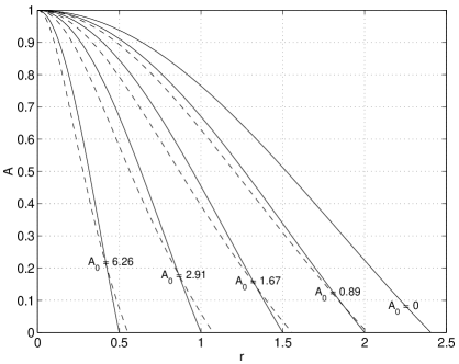
Figure 1: Comparison of the variational results (solid lines) to the numerical ones (dashed lines) for a focusing nonlinearity.

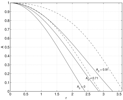
Figure 2: Comparison of the variational results (solid lines) to the numerical ones (dashed lines) for a defocusing nonlinearity.

We now turn to an investigation of the overall behaviour of the nonlinear Bessel beam profiles. The fact that the main influence of the nonlinear term is a rescaling of the radial coordinate makes it reasonable to look for an approximate solution of the form

$$A(r)\approx A_{0}J_{0}(f(r)),$$ (16)

where $f(r)$ is a function of $r$, $\delta$, $\kappa$, and $A_{0}$. It is difficult to determine $f$ using analytical methods, but by noticing that the linear solution can be written as

$$A=A_{0}J_{0}\left(\int_{0}^{r}\sqrt{\delta}\d r^{\prime}\right),$$ (17)

and by comparing with Eq. (5) it seems reasonable that a good approximation should be obtained by the implicit expression

$$A=A_{0}J_{0}\left(\int_{0}^{r}\sqrt{\delta+\kappa A^{2}(r^{\prime})}\d r^{\prime}\right).$$ (18)

Although this is, in fact, an integral equation for $A(r)$, it nevertheless provides a very simple formula for finding $A$ numerically. The corresponding approximate solution is compared to the numerical solution of the full equation in Fig. 3. When the amplitude is low the two curves are identical, since the ansatz then reduces to the Bessel function. In the case of a focusing nonlinearity, there is good agreement between the two approaches, but it is also seen that a phase shift appears between the curves for increasing $A_{0}$. Quite good agreement is seen also in the defocusing case. In particular, the initial flattening is well modelled. The phase shift is now of the opposite sign.

This approximate solution implies that the argument of the Bessel function increases approximately as $\int_{0}^{r}\sqrt{\delta+\kappa A^{2}}\d r^{\prime}$, which is a nonlinear generalisation of the linear case. Thus the main effect of a focusing nonlinearity is to increase the curvature of the peaks by increasing the growth rate of the argument, making the solution radially compressed. In the defocusing case the curvature is decreased, which is most clearly seen in the main lobe.

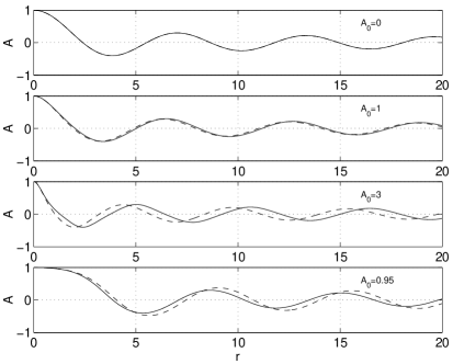
Figure 3: The implicit analytical solution given by Eq. (18) (solid lines) together with the numerical result (dashed lines). The different initial amplitudes are indicated in the graph. A defocusing nonlinearity is used in the fourth plot.

Finally, Figs. 4 and 5 further illustrate the nonlinear deformations of the linear diffraction-less Bessel solutions. The numerically obtained curves clearly show the features discussed above; the radial compression of the central lobe in the focusing case and the radial expansion in the defocusing case. The expansion effect in the latter case rapidly increases as the amplitude approaches the critical value $A_{0}=1$, above which no stationary solutions are possible. The phase shifting effect of the nonlinearity on the Bessel-like oscillations is also seen, the shift changing sign with the sign of the nonlinearity.

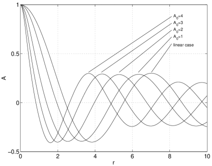
Figure 4: A focusing nonlinear term gives rise to a radial compression, which is illustrated using numerical simulations.

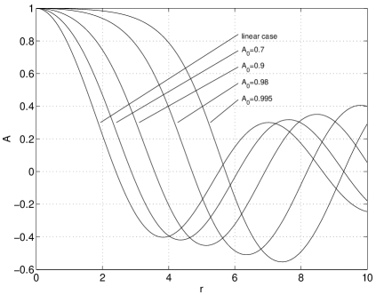
Figure 5: Numerical solutions showing the influence from a defocusing nonlinear term.

4 Analysis of nonlinear Bessel-Gauss beams

The linear diffraction properties of Bessel-Gauss beams have been analysed and solved analytically, see [3]. In the present section we will analyse the nonlinear dynamics of beams, which initially have a profile in the form of a Bessel function truncated by a Gaussian. Since a general solution of this problem cannot be given, we will use the virial theorem to obtain analytical information and numerical simulations for determining the evolution of the beam profile.

The virial theorem, see e.g. [13, 14, 15], provides exact and explicit information about the dynamic variation of the width of the beam, $\sigma$, defined in the RMS sense as $\sigma^{2}\equiv\langle r^{2}\rangle$, where

$$\langle f(r)\rangle\equiv\frac{\int_{0}^{\infty}f(r)|\psi(z,r)|^{2}r\d r}{\int_{0}^{\infty}|\psi(z,r)|^{2}r\d r}.$$ (19)

The virial theorem asserts that

$$\frac{d^{2}\sigma^{2}}{dz^{2}}=8\frac{H}{I}=\mbox{constant},$$ (20)

where $I$ and $H$ are invariants of the two-dimensional nonlinear Schrödinger equation, Eq. (1), and are defined as follows

$$I = \int_{0}^{\infty}|\psi(z,r)|^{2}r\d r,$$ (21)

$$H = \int_{0}^{\infty}\left[\left|\frac{\partial\psi(z,r)}{\partial r}\right|^{2}-\frac{\kappa}{2}|\psi(z,r)|^{4}\right]r\d r.$$ (22)

This means the invariants correspond to the (integrated) beam intensity and the Hamiltonian. Thus, the virial theorem implies that $\sigma^{2}$ must be a second order polynomial in $z$, with coefficients determined by the initial beam profile, $\psi(0,r)$. For initial phase functions that do not depend on $r$, the linear term in $z$ vanishes, and the beam width varies as

$$\sigma^{2}(z)=\sigma^{2}(0)\left(1+\operatorname{sign}(H)\frac{z^{2}}{L_{0}^{2}}\right)$$ (23)

where $L_{0}$ is a characteristic length given by

$$L_{0}^{-2}=\left|\frac{4H}{\sigma^{2}(0)I}\right|=\left|\frac{4\int_{0}^{\infty}\left[\left|\frac{\partial\psi(z,r)}{\partial r}\right|^{2}-\frac{\kappa}{2}|\psi(z,r)|^{4}\right]r\d r}{\int_{0}^{\infty}r^{2}|\psi(0,r)|^{2}r\d r}\right|.$$ (24)

Clearly this approach cannot be used for analysing the linear, or the nonlinearly modified, stationary Bessel beam solutions of the nonlinear Schrödinger equation since all integrals involved in the virial theorem are infinite. However, for a physical beam, with finite integral content, the virial theorem is useful. In general it is seen that with weak nonlinear focusing effects, the Hamiltonian is positive and the RMS width will increase quadratically with a characteristic diffraction length given by $L_{0}$. When the amplitude of the beam increases, the Hamiltonian decreases and eventually changes sign. This implies that the RMS width goes to zero after a finite length equal to $L_{0}$—the well known nonlinear collapse phenomenon, where $L_{0}$ now plays the role of collapse length.

For Bessel-Gauss beams, [3], the initial profile is of the form

$$\psi(0,r)=A_{0}J_{0}\left(\frac{r}{r_{0}}\right)\exp\left(-\frac{r^{2}}{2\rho_{0}^{2}}\right).$$ (25)

Inserting this into Eq. (24) we obtain the following expression for the characteristic length $L_{0}$

$$\left(\frac{r_{0}}{2L_{0}}\right)^{2}=\frac{S_{1}(\mu)-\Lambda S_{2}(\mu)}{S_{3}(\mu)}$$ (26)

where $\mu=r_{0}^{2}/\rho_{0}^{2}$, $\Lambda=\kappa A_{0}^{2}r_{0}^{2}$, and the integrals $S_{n}$, $n=1,2,3$, are given by

$$S_{1}(\mu) = \int_{0}^{\infty}[\mu xJ_{0}(x)+J_{1}(x)]^{2}\exp(-\mu x^{2})x\d x,$$ (27)

$$S_{2}(\mu) = \int_{0}^{\infty}J_{0}^{4}(x)\exp(-2\mu x^{2})x\d x,$$ (28)

$$S_{3}(\mu) = \int_{0}^{\infty}x^{2}J_{0}^{2}(x)\exp(-\mu x^{2})x\d x.$$ (29)

Since we are primarily interested in the case when the Gauss function truncates the outer parts of the Bessel function, we have $\mu=r_{0}^{2}/\rho_{0}^{2}\ll 1$. In this limit, the asymptotic values of the integrals, $S_{n}$, $n=1,2,3$, are obtained analytically as

$$S_{1}(\mu) \approx \frac{1}{2\sqrt{\pi}}\frac{1}{\sqrt{\mu}},$$ (30)

$$S_{2}(\mu) \approx D_{1}-\frac{3}{4\pi^{2}}\ln\mu,$$ (31)

$$S_{3}(\mu) \approx \frac{1}{4\sqrt{\pi}}\frac{1}{\mu^{3/2}},$$ (32)

Since $S_{2}(\mu)$ goes rather slowly towards infinity as $\mu$ becomes small, it is necessary to determine the constant $D_{1}$ in order to have good accuracy for finite $\mu$. Using numerical evaluation of the integral we find $D_{1}\approx 0.202$. This implies that the characteristic length can be approximated as

$$\left(\frac{r_{0}}{2L_{0}}\right)^{2}\approx 2\mu\left[1-\Lambda\sqrt{\mu}\left(D_{2}-\frac{3\ln\mu}{2\pi^{3/2}}\right)\right],$$ (33)

with $D_{2}\approx 0.715$. In the linear case, the characteristic length is seen to scale simply as $L_{0}\propto\rho_{0}$, i.e., the diffraction is determined solely by the truncation radius and as $\rho_{0}\to\infty$, the non-diffracting Bessel beam is recovered. For increasing values of the nonlinearity parameter, $\Lambda$, but for a fixed truncation radius, the value of $L_{0}$ increases and for a certain critical value of $\Lambda$, the nonlinearity balances the diffraction to give a Bessel-Gauss beam, which is diffraction-less in the RMS sense.

5 Dynamics of Bessel-Gauss beams

When a truncated linear Bessel-Gauss beam propagates, the diffraction initially affects only the outermost part of the pulse, where the truncation has changed it from the Bessel shape. The central parts are initially diffraction balanced and remains so until the “diffraction front” propagating inwards from the outer parts eventually reach the inner lobes and also these parts start to diffract outwards. On the other hand, the nonlinear effect is strongest at the centre of the beam, where the intensity is highest, and with a focusing nonlinear term, the main lobe will start to compress. In fact, it will start to compress irrespective of the degree of nonlinearity since the linear diffraction is already balanced. If the nonlinear effect is weak the compression will eventually stop, and diffraction will become the dominating effect. This evolution is illustrated in Fig. 6, where an FDTD simulation using $A_{0}=1$ and $\mu=0.01$ is shown. Although the central parts initially compress, the virial theorem predicts beam broadening in the RMS sense. Clearly this is no contradiction since the broadening of the outer parts more than compensate the compression of the centre. In order to further illustrate how the main lobe is compressed, the intensity at $r=0$ has been plotted for different initial amplitudes as a function of propagation distance in Fig. 7. The curves have been normalised with respect to their amplitudes at $r=0$ and $\mu=0.01$. We emphasise the oscillating behaviour for the highest amplitudes. If the nonlinear effect is sufficiently strong, the virial theorem predicts a collapse of the beam to zero RMS width. According to Eq. (33), the amplitude threshold for this type of behaviour is $A_{0}>A_{c}\approx 2.26$ for $\mu=0.01$. It is well known that the nonlinear evolution of two-dimensional beams may lead to a break up of the beam into a diffracting background profile with a monotonously compressing filament, that collapses in a finite distance of propagation. Thus, the width of the filament goes to zero and the intensity becomes infinite whereas the beam width in the RMS sense still increases. The simulations for the present case of Bessel-Gauss beams show that when the amplitude is increased further above $A_{0}=1$, the small second peak of Fig. 7 will start to dominate and eventually the simulations indicate a collapse of the second peak, although the RMS width still tends to infinity. In fact, even if the RMS width remains constant, the beam should still be able to undergo partial collapse.

Much effort has been devoted to the study of two-dimensional collapse phenomena induced by the Kerr nonlinearity, see e.g. [13, 14, 15] and references therein. In particular, it has been found that the virial theorem poses a sufficient but not necessary condition for the occurrence of a singularity where the amplitude becomes infinite. Thus the appearance of a partial collapse singularity below the threshold for a global collapse, as predicted by the virial theorem, is in accordance with earlier results.

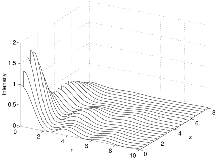
Figure 6: An example of the evolution of the radial intensity profile with distance of propagation.

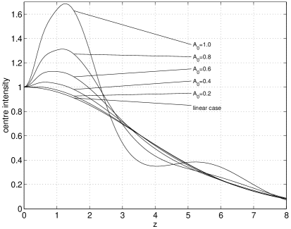
Figure 7: The intensity at $r=0$ as a function of the propagation distance using different initial amplitudes.

6 Conclusions

Based on the nonlinear Schrödinger equation in cylindrical geometry we have studied the modification of the diffraction-less linear Bessel beams caused by the nonlinear Kerr effect. The stationary as well as the dynamic properties of the solutions to this equation have been analysed and both analytical and numerical techniques have been used. The investigation shows that the nonlinearity primarily affects the main and inner lobes of the Bessel beams. In the case of the stationary solutions, the central region of the nonlinear Bessel beam tends to become radially more narrow or more extended depending on whether the nonlinearity is focusing or defocusing, respectively. Asymptotically the solutions are still of the same oscillating form as the diffraction-less Bessel beams, the only remaining feature of the nonlinearity being a phase shift as compared to the linear case. However, in the case of the defocusing nonlinearity, there is a finite amplitude threshold for well-behaved solutions to exist. Above this limit the nonlinear diffraction effect becomes larger than the linear effect, which counteracts the diffraction, and no solutions are possible which vanish at infinity.

The properties of Gaussian-truncated Bessel beams have also been studied in the presence of the Kerr nonlinearity. It has been shown, using the virial theorem, that a non-diffracting situation in the RMS sense is possible to obtain by balancing nonlinear focusing and linear diffraction. However, this situation does not correspond to a stationary case of the beam profile. Significant redistribution of the beam occurs and using numerical simulations, the dynamic interaction between linear diffraction and nonlinear focusing has been analysed for varying degrees of nonlinearity. It has been found that, in particular the central parts of the beam may become significantly distorted and may even partially collapse even though the beam width, defined in the RMS sense, remains constant or even increases. This result is in agreement with the classical picture of dynamic self focusing of two-dimensional beams in nonlinear Kerr media.

References

- [1] J. H. Marburger, Progress in Quantum Electronics 4 (1975) 35.
- [2] J. Durnin, Journal of the Optical Society of America A 4 (1987) 651.
- [3] F. Gori, G. Guattari, C. Padovani, Optics Communications 64 (1987) 491.
- [4] P. Sprangle and B. Hafizi, Comments on Plasma Physics and Controlled Fusion 14 (1991) 297.
- [5] S. Sogomonian, S. Klewitz, S. Herminghaus, Optics Communications 139 (1997) 313.
- [6] D. Ding, S. Wang, Y. Wang, Journal of Applied Physics 86 (1999) 1716.
- [7] R. Gadonas, V. Jarutis, R. Paškauskas, V. Smilgevičius, A. Stabinis, V. Vaičaitis, Optics Communications 196 (2001) 309.
- [8] R. Butgus, R. Gadonas, J. Janusonis, A. Piskarkas, K. Regelskis, V. Smilgevičius, A. Stabinis, Optics Communications 206 (2002) 201.
- [9] N. R. Pereira and L. Stenflo, The Physics of Fluids 20 (1977) 1733.
- [10] D. Anderson, F. Cattani, M. Lisak, Physica Scripta T82 (1999) 32.
- [11] R. Y. Chiao, E. Garmire, C. H. Townes, Physical Review Letters 13 (1964) 479.
- [12] D. Anderson, M. Bonnedal, M. Lisak, Physics of Fluids 22 (1979) 1838.
- [13] J. Juul Rasmussen and K. Rypdal, Physica Scripta 33 (1986) 481.
- [14] K. Rypdal and J. Juul Rasmussen, Physica Scripta 33 (1986) 498.
- [15] G. Fibich and G. Papanicolaou, Journal of Applied Mathematics and Physics 60 (1999) 183.