The VLQ Calorimeter of H1 at HERA:
A Highly Compact Device for Measurements of Electrons and Photons under Very Small Scattering Angles

Abstract

In 1998, the detector H1 at HERA has been equipped with a small backward spectrometer, the Very Low Q² (VLQ) spectrometer comprising a silicon tracker, a tungsten - scintillator sandwich calorimeter, and a Time-of-Flight system. The spectrometer was designed to measure electrons scattered under very low angles, equivalent to very low squared four - momentum transfers $Q^{2}$, and high energy photons with good energy and spatial resolution. The VLQ was in operation during the 1999 and 2000 run periods. This paper describes the design and construction of the VLQ calorimeter, a compact device with a fourfold projective energy read-out, and its performance during test runs and in the experiment.

1 Introduction

1.1 Physics Motivation

The storage ring HERA at DESY where electrons or positrons of 27.5 GeV collide with protons of 920 GeV is devoted to the investigation of deep inelastic electron - proton scattering (DIS) and photoproduction processes. The detector H1 [1] at HERA is equally well equipped for measuring electrons scattered in deep inelastic, i.e. high $Q^{2}$, reactions, by virtue of its Liquid Argon (LAr) [1] and SpaCal [2] calorimeters, and electrons which initiated photoproduction, i.e. $Q^{2}\approx 0$, reactions with the help of its low angle (w.r.t. the electron beam direction) electron spectrometers, called the “electron taggers”.

However, the available range in $Q^{2}$ which is linked to the electron’s scattering angle is limited by the inner radius of the SpaCal which corresponds to a minimal $Q^{2}$ of roughly 0.6 GeV². Therefore, a large area in phase space cannot be accessed by H1 without the help of a dedicated device, see Fig. 1 which shows the acceptance range of H1 in a $Q^{2}-y$ map. The variable $y$ is, for vanishing $Q^{2}$, defined by $~{}y=1-E^{\prime}/E~{}$ where $E$ is the energy of the incoming, $E^{\prime}$ that of the scattered electron. Therefore, $y~{}=~{}0$ corresponds to vanishing, $y~{}=~{}1$ to maximal photon energy. The region below the SpaCal - covered $Q^{2}$ range is of special interest because here the DIS and photoproduction regimes merge: The “transition region”. A measurement of the structure function $F_{2}(W^{2},Q^{2})$, or equivalently of the total photo-absorption cross section

$$\sigma(\gamma^{*}p)=4~{}\pi^{2}~{}\alpha/Q^{2}~{}F_{2}(W^{2},Q^{2}),$$

in this region is expected to shed light on the interplay between soft and hard processes in electron - proton scattering. The VLQ extends the kinematically accessible range down to values of $Q^{2}=0.03$.

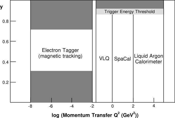
Figure 1: The acceptance region of H1 in the $y$ - $Q^{2}$ plane.

Furthermore, a measurement of vector meson production in this regime, especially a comparison between cross section behaviours for the production of light ($\rho^{0}$, $\omega$, $\phi$) and heavy (J/$\psi$, $\Upsilon$) mesons, in the transition region will help to improve the understanding of strong interaction mechanisms [3].

The VLQ calorimeter, which does not distinguish between high energy electrons and photons, can also serve to measure photons from meson decays, e.g. from $\pi^{0}$ or $\eta$ mesons, or from heavier particles which decay through these intermediate states. A field which gained new interest is meson production via “Odderon” exchange, where the Odderon is the $P=C=-1$ partner of the Pomeron. Odderon - mediated reactions are expected to lead to high energy single meson production in the “photon hemisphere”, that is in the electron beam direction [4]. The VLQ is an ideal target for photons from these meson decays [5].

1.2 Detector Design: Constraints and Concept

The VLQ spectrometer consists of two independent modules, each comprising a tracker system and an electromagnetic calorimeter, followed by a time-of-flight (ToF) system which has the purpose to recognize background particles travelling along with the proton beam. The phase space region to be covered dictates the position of the VLQ to be downstream the electron beam and close to the beam pipe. The space available to install a new detecting device there is strongly limited, enforcing a very tight structure, and especially a highly compact calorimeter. The solution chosen is a system of two identical spectrometer modules, one above and one below the beam line, fixed to a moving mechanics so that the modules can be moved close to the beam, or retracted, independently. The tracker part and the ToF system connected to the VLQ spectrometer are described in [6].

The volume available for either VLQ calorimeter module is a box of 16.3 cm length and transverse dimensions of 15.0 x 18.0 cm². The calorimeter operates in an energy range up to the electron beam energy, i.e. roughly 30 GeV. The energy resolution aimed at in this regime is 3 - 4 %. A material capable to absorb electromagnetic showers of this energy within the given distance is tungsten, with Z = 72 and a density of 19.3 g/cm³. A sandwich calorimeter type was chosen in a sophisticated layout which allows a “projective energy read-out”, i.e. a fourfold projection of the shower profile can be measured along the shower detector: A passive tungsten  plate of 2.5 mm thickness is followed by an active scintillator layer of 3 mm thickness, structured in an array of 24 vertical scintillator bars of 5 mm width each; this double layer is continued by another tungsten plate and another scintillator layer, arranged in 18 horizontal scintillator bars of the same width. In total there are 23 tungsten and 24 scintillator layers. The scintillation light which is guided by total reflection is read out at either end of each bar, and coupled into a wavelength shifter which guides the light towards photodiode detectors.

2 Calorimeter Design and Construction

2.1 Design Parameters and Optimization

Detection devices positioned very close to the beam pipe are exposed to high doses of synchrotron radiation and background generated by the proton beam. In order to protect the VLQ from background radiation, a moving mechanism retracts the spectrometer from the beam pipe during the filling phase. This condition renders a full $2\pi$ coverage in azimuth more difficult and leaves a two module solution: One module above, and another identical one below the beam pipe, fixed to the retraction mechanism which moves the modules to well defined measuring positions. The parameters of the calorimeter described below always refer to a pair of modules. The structure of a calorimeter module is sketched in Fig. 2 , an “exploded view” is shown in Fig. 3.

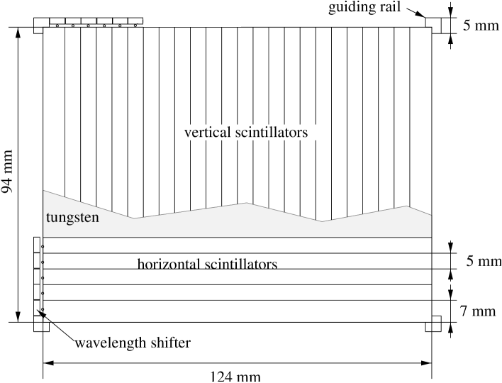
Figure 2: Front view of the calorimeter structure.

The scintillation material chosen is Bicron BC-408 with a wavelength of maximum emission of 425 nm, a decay time of the scintillation light of 2.1 ns, and a refractive index of 1.58 [7].

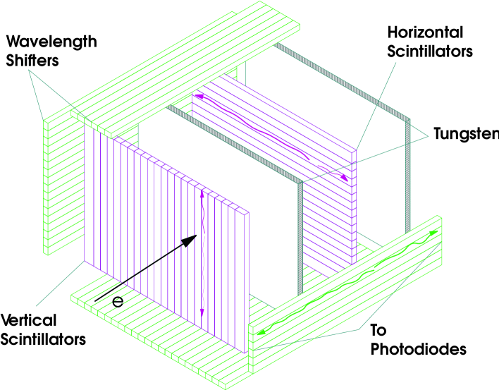
Figure 3: “Exploded view” of a calorimeter module.

Given the available space and the absorber and scintillator materials, the internal structure of the calorimeter module has to be optimized. The total length being fixed, the parameters to be varied are number and thickness of tungsten vs. scintillator plates. The optimization procedure was carried out using the simulation package GEANT [8]. The optimization criterion is derived from the behaviour of the relative energy resolution $\sigma(E)/E$ which is conventionally expanded in powers of $1/\sqrt{E}$:

$$\sigma(E)/E=S/\sqrt{E}\oplus C\oplus N/E.$$ (1)

Here, $S/\sqrt{E}$ is the so called “sampling term” governed by Poisson statistics of shower sampling. $C$ is called the “constant term” saying that the absolute energy resolution $\sigma(E)$ worsens with increasing energy. It is mainly due to incomplete shower containment and strongly dependent on the calorimeter size. $N/E$ is the noise term which is not a property of the calorimeter body itself but given by the readout system. It has the same influence on the absolute resolution at any energy, i.e. it is independent of energy.

Optimization of the mechanical layout of the calorimeter can be decoupled from the electronic read-out [9]. To find the best solution, a series of simulations was performed where the tungsten and scintillator layer thicknesses were varied [9]. The electron impact energies were 5, 15 and 25 GeV. A curve corresponding to eq. 1 was fit to the simulated energy distribution without the noise term which has not been simulated. The optimal solution, a tungsten layer thickness of 2.5 mm and a scintillator layer thickness of 3 mm, resulted in the following expression for the energy resolution:

$$\frac{\sigma(E)}{E}=\sqrt{\left(\frac{12.9\%}{\sqrt{E/\text{GeV}}}\right)^{2}\oplus(3.2\%)^{2}}.$$ (2)

A parameter for the noise term could not be derived from the simulation but was obtained from an independent investigation of the read-out chip, see [9, 10] and below (Section 2.4).

An equivalent investigation was made in order to determine the optimal width of the scintillator strips. A good spatial resolution is clearly in favour of a small width, but implies a larger number of read-out channels and a smaller light yield per scintillator, with increased relative noise contributions. The compromise found was a width of 5 mm resulting in a (one dimensional) spatial resolution of 1.4 mm at 5 GeV. The resolution improves to below 1 mm for higher energies due to reduced shower fluctuations.

Another important property of any calorimeter is the relation between input energy and measured response. Deviations from linearity lead to systematic uncertainties and deteriorate the effective energy resolution. The simulation study on the optimized VLQ calorimeter shows deviations from linearity below one percent which are a consequence of the compactness of the calorimeter body and corresponding leakage effects at high energies, see Fig. 4.

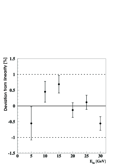
Figure 4: Deviation of calorimeter response from linearity in the energy range from 5 to 30 GeV. Result of simulation.

Following the simulation results, the calorimeter in its structure as described above represents an “electromagnetic depth” of 16.7 radiation lengths and has a Molière radius (the radius of a cylinder containing on the average 90 % of the shower energy) of 1.25 cm.

2.2 Mechanical Layout

The two modules of the calorimeter need to be retracted during the beam filling phase in order to protect the silicon tracking device from synchrotron and background radiation. With the help of the moving mechanics, the radiation load of the VLQ tracking system can be reduced by a factor of more than 20. The moving apparatus delivers a (vertical) position information which is read out and continuously stored after every move-in / move-out procedure. Its accuracy is of the same order as that of the tracker, i.e. a few $\mu$m.

The VLQ calorimeter modules, including the electronic read-out systems, are accomodated in a solid brass housing each, with wall thicknesses of 8 mm (side walls), 5 mm (front and back walls), and 2 mm (bottom wall, i.e. the wall closest to the beam pipe). Thus, sufficient protection against synchrotron radiation is provided. Inside a module, another 10 mm thick brass plate is mounted directly above the active volume which accomodates the cooling water tubing system: The water serves to cool an air stream which continually flows around the electronics boards. The tracker modules are fixed to the calorimeter modules, as sketched in Fig. 5.

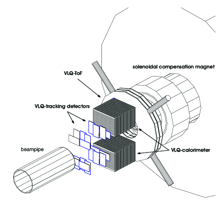
Figure 5: Sketch of the mechanical layout of the VLQ (tracker, calorimeter, ToF).

The VLQ spectrometer is situated as close to the beam line as possible in order to catch electrons and photons scattered or produced at very small angles. This requires a modification to the beam pipe because even a thin but straight cylindrical pipe would force particles to traverse a large amount of material. The shape of the beam pipe with its changing diameter is shown in Fig. 6. The pipe is made of aluminium, and the material in front of the VLQ corresponds to less than one radiation length.

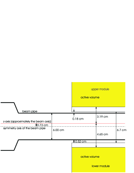
Figure 6: Sketch of the beam pipe shape in front of the VLQ spectrometer.

2.3 Light Transport and Collection

After the considerations sketched above, the structure and granularity of the scintillation and light transport system are fixed: The calorimeter has 24 scintillator layers, 12 vertically and 12 horizontally structured ones. Each vertically structured layer consists of 24 bars, each horizontally structured one consists of 18 bars. An exploded view of the calorimeter structure is displayed in Fig. 3 . The active, scintillating layers are interleaved with 23 passive, tungsten layers. The very first and very last passive layer are represented by the front and back brass housing walls.

Each scintillator strip is read out at either side by a wavelength shifter (WLS) bar [11] which collects and sums the light from 24 strips: In total, there are 2 x (18 + 24) = 84 WLS bars per module. Each WLS bar is read out by a photodiode at either end so that 168 photodiodes are needed per module. Each surface plane of a calorimeter module is read out in this manner, so that four independent transverse shower projections are available.

The wavelength shifters are located close to each other with a distance of only 0.2 mm. Consequently, the use of a single photodiode with its own housing for an individual WLS is not possible. Instead, especially manufactured photodiode arrays which match the dimensions of the WLS arrays were employed . There are two kinds of arrays, one with 18 and one with 24 diodes, each implanted in a common p - substrate, corresponding to the transverse structure of the calorimeter with its two different sets of read-out channels. The size of the active area of a single diode is 4.2 x 3.4 mm². The distance between the active areas is 0.8 mm. The diode arrays are protected by a glass surface of 0.5 mm thickness.

The determination of shower energy and shower position is based on the evaluation of the transverse shower profiles. Any effect which disturbs the primary “physical” profile has to be avoided or at least minimized. One such effect ist optical cross talk between adjacent scintillator strips: Scintillation light induced in one channel reaches neighbouring ones and thus distorts the primary profile. To avoid this, each scintillator strip was wrapped in individually prepared and cut white paper.

Each scintillator strip matches with either end its WLS bar. Scintillator and WLS have the same refractive index (n = 1.58) so that an intimate contact would be desirable to minimize light losses. Since this contact could only be established manually by gluing which inevitably leads to non-uniform connections, scintillator and WLS were separated by a 0.2 mm wide gap which is maintained by a Nylon thread. The WLS strips guide the light directly onto the photodiode surfaces.

Scintillator and WLS materials are selected to match the sensitivity and quantum efficiency of the photodiodes. The scintillator’s wavelength of maximum emission is 425 nm; its light is shifted by 100 nm towards larger wavelengths (from “blue” to “green”) when re-emitted by the WLS. The photodiode reaches a modest sensitivity but high quantum efficiency at this wavelength, see Fig. 7.

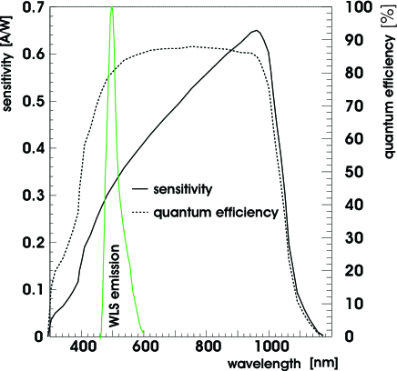
Figure 7: Response curves of the Hamamatsu PIN photodiode.

Finally, the glue between WLS and glass surfaces (n = 1.50) of the photodiodes was chosen as an Epoxid resin with a refractive index of n = 1.56 which means nearly optimal matching. Its transparency in the wavelength range of the WLS is larger than 99 %.

The attenuation length of a scintillator slab of dimensions 1 x 20 x 200 cm³ is 210 cm [7]. This changes drastically for scintillator strips of dimensions used for the VLQ calorimeter, namely 3 x 5 x 90 (120) mm³. In these very thin strips the number of reflections which scintillation light undergoes, and consequently the net light loss, is much larger. A measurement of the attenuation [12] results in a parametrization by a sum of two exponential functions: The region close to the exit surface is governed by a very small attenuation length of 2.7 mm, the region towards the scintillator centre is described by an attenuation length of 101 mm.

The efficiency of light transmission from scintillators to wavelength shifters is between 80 % and 90 %, the light collection efficiency of the WLS is about 50 % [9]. In total, a fraction of 5 - 10 % of the light induced by an electromagnetic shower is collected onto the photodiodes.

A survey of the technical parameters of the VLQ calorimeter is given in Table 1.

Length	16.3 cm
Width	18.0 cm
Height	15.0 cm
Volume	4.4 l
Mass	14.2 kg
No. of tungsten layers	23
No. of scintillating layers	24
No. of hor. scintillating bars/layer	18
No. of vert. scintillating bars/layer	24
No. of hor. scintillating bars	216
No. of vert. scintillating bars	288
No. of photodiodes	168
Width of scintillating bars	5.0 mm (4.8 mm)
Thickness of tungsten layers	2.5 mm
Thickness of scintillating layers	3.0 mm
Length of active volume	13.9 cm
Mean density	8.55 g/cm3
Depth (X0)	6.7
Molière radius (Design)	1.25 cm

Table 1: Technical Parameters of the VLQ Calorimeter.

2.4 Electronic Read-out

The read-out via photodiodes requires an electronic amplification of the diode signals. An energy deposition of 5 GeV in the calorimeter liberates roughly 55000 electrons in the photodiodes. Since these photoelectrons are generally distributed over several detecting diodes, a charge corresponding to 1000 electrons has to be measured well above noise. This condition imposes demanding requirements on the read-out circuit, especially in terms of electronic noise. The terminal capacitance of a single diode in the array is 10 pF when operated at a bias voltage of 70 V.

The read-out of the photodiodes is performed via charge sensitive preamplifiers realized as full custom Application Specific Integrated Circuits (ASICs), for reasons of compactness and power consumption. The preamplifier chips are mounted with Chip On Board (COB) Technology, on the front and back printed circuit boards (PCB) of the calorimeter structure directly behind the photodiodes, in order to avoid additional capacitive loading of the preamplifier inputs through connecting wires. The amplified diode signals are brought to a top PCB where summing amplifiers and differential line drivers are located. The preamplifier chip was specifically designed and produced in the Austria Micro Systems (AMS) 1.2 $\mu$m CMOS process. It features six preamplifier channels with subsequent shaping, fast trigger summing (see Section 2.5) and an on-chip charge calibration system. The rise time of the preamplifier output is 30 ns followed by a 200 ns shaping. Principally, the noise goes down with increasing shaping time. On the other hand, the probability of overlapping events increases due to the HERA bunch crossing distance of only 96 ns. A shaping time of 200 ns was chosen as a compromise. The read-out chain and the scheme of the read-out chip circuit are shown in Fig. 8 and Fig. 9.

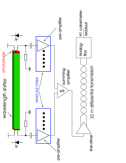
Figure 8: Read-out channel scheme.

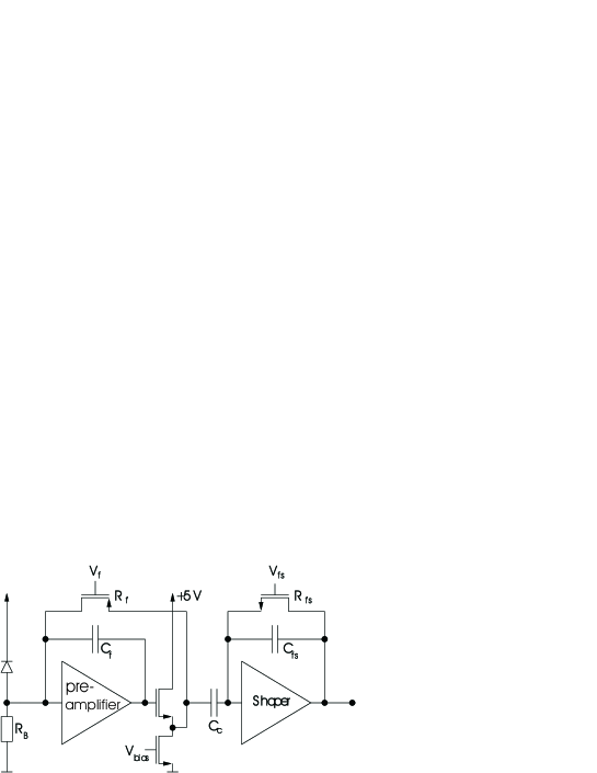
Figure 9: Read-out chip circuit scheme.

The noise of the shaped signal affects energy and spatial resolutions of the calorimeter. The measured noise of the chip amounts to 226 + 19 x $C$(pF) electrons r.m.s. where $C$ represents the capacitive load. Fig. 10 shows the noise measured at the output of the charge amplifier of the read-out chip as a function of the capacitance at the input.

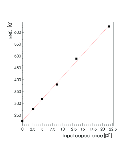
Figure 10: Measured noise (in ENC) as a function of the preamplifier input capacitance.

With the photodiodes used here, this corresponds to an effective noise figure of 416 electrons r.m.s. With an estimated signal of 11 000 electrons for a 1 GeV electron shower out of which 75 % are deposited in a core seen by two horizontal and two vertical scintillator bars with front and back read-out, a calibrated noise figure of 120 MeV is anticipated.

After shaping, the two signals from either end of one WLS bar are summed and sent, through a 30 m long cable, differentially to the analogue receivers located in the electronics hut of the H1 experiment This system is identical to that one operated in the read-out of the H1 backward calorimeter BEMC [13]. The read-out and amplification electronics, including the line driver, are located inside the VLQ calorimeter housing. The total power consumption of 25 W is mainly due to the line drivers, and requires water cooling of the read-out electronics.

The calorimeter signals are re-transformed into unipolar signals by a differential receiver. The signal is delayed by 2.2 $\mu$s with the help of an adjustable analogue delay line. This time is needed to store the signals until the first level trigger of the H1 detector has made a decision. The signals from this analog pipeline are amplified once more and, in case of a positive trigger decision, stored in a Sample-and-Hold circuit as analog voltages. The Sample-and-Hold circuit stores the voltage at exactly that time when the trigger signal arrives. This requires a precise timing of the calorimeter signals whose maxima are to be stored upon trigger signal arrival.

One analog receiving card accomodates 16 equally built channels. The voltages stored in these 16 Sample-and-Hold circuits are, after trigger decision, transferred via a multiplexer to the H1 standard calorimeter read-out system [14] where signals are digitized in a 12 bit ADC , and stored. In this way, the 84 signal and 4 trigger channels of a calorimeter module are read out. The trigger channels are also fed into the analog read-out in order to perform trigger control measurements.

2.5 The Calorimeter Trigger

The VLQ spectrometer is devoted to new physics regimes where high energetic particles are scattered through small angles into the backward region of H1, i.e. the region downstream the electron beam. The VLQ becomes therefore an important and independent element of the H1 trigger system.

A VLQ calorimeter trigger signal can carry information on energy deposited, above a certain threshold, in a certain section of the calorimeter. A maximum number of four trigger signals per module is possible as dictated by the resources of the H1 Central Trigger Logics (CTL). The signal has to be derived from the (2 x 18) + (2 x 24) read-out channels available. The most simple conceivable trigger signal would be just the sum of the signals of all read-out channels. This straight - forward solution has two drawbacks: First, since an electromagnetic shower distributes its energy over few channels only, signals are added from calorimeter regions “far away” from the shower, thus adding just noise to the sum signal. Second, a rather frequently occurring background effect known as “Single Diode Effect” (or “Nuclear Counter Effect”) would not be suppressed in such a simple scheme.

The calorimeter noise can be separated into two classes: Coherent and incoherent noise. The former is due to signals, e.g. out of the electronic environment, which are picked up by all calorimeter channels simultaneously. They will lower or raise the original signals by roughly the same amount. Incoherent noise is individual (e.g. statistically generated) activity, with a Gaussian amplitude spectrum centered at zero whose spread is supposed to be reduced when summed over. The contribution from coherent noise is proportional to the number of noisy channels, the contribution from incoherent noise to its square root. To minimize the noise contribution, in particular from coherent noise, the number of channels to be summed up to yield a signal must be kept as small as possible.

The “Single Diode” (SD) effect is generated by particles passing through the depletion layer of a diode and leaving an amount of energy which mimics a high energy shower signal.

The suppression of both coherent noise and SD effect require a more segmented trigger scheme because the “total sum” solution would lead to an intolerable trigger threshold behaviour, and suppression of SD events needs comparison of channels opposite to each other. Therefore, in a first step only calorimeter signals from horizontal scintillator bars, read out at the vertical sides, are used for triggering. They suffer less strongly from the SD effect because the calorimeter regions close to the beam line, and thus the corresponding horizontal photodiode arrays, are much more frequently hit by scattered electrons due to their $1/Q^{4}$ (i.e. Rutherford) angular distribution.

In a second step, the calorimeter module is logically divided into trigger segments. Vertically, two windows are constructed of nine channels each, with an overlap of six channels. The overlap region is chosen large enough to cover a complete shower which deposits nearly all its energy in one central plus two left and two right neighbouring channels. The trigger efficiency is thus not reduced for particles impinging close to the edge of a window. The trigger pattern is shown in Fig. 11.

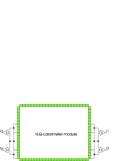
Figure 11: The VLQ calorimeter geometrical trigger pattern.

Each vertical window is read out at either side so that “left signal” and “right signal” can be compared. As the light attenuation in the scintillator strips is weak, a real shower should lead to roughly equal signals at either side, while SD events do not, and thus can easily be recognized at the trigger level.

The outmost six channels (which point towards the main detector) are not included in the trigger because they are hidden in the shadow of the SpaCal insert [2] which was supposed to be modified in a later upgrade step. The trigger scheme is, as is the read-out scheme, symmetrical for both modules. In summary, four analog trigger signals per module, or eight signals for the entire spectrometer, are available.

The analog trigger signals are delivered to the trigger module which prepares the digital trigger information. First, the analog signals from opposite sides of a window are added in order to avoid inhomogeneities in the trigger efficiency. In addition, thresholds are applied to the eight original sums yielding the signals N1 to N8; these (low) thresholds are labelled “noise triggers”. Furthermore, two independent (“low” and “high”) thresholds are applied to the newly built sums, yielding another eight digital signals (L1+3 to L6+8, H1+3 to H6+8). These digital signals are synchronized with the HERA clock on the trigger module. The 16 digital signals generated on the trigger module are fed into a general purpose digital input - output card. It accomodates a freely programmable look-up table which combines the input signals to the eight VLQ trigger elements delivered to the Central Trigger Logics of H1. All thresholds in the trigger module can be adjusted individually.

Finally, there are eight VLQ - derived trigger elements, four derived from the top module, and four derived from the bottom module. For symmetry reasons, only the four top - derived elements are explained here:

“VLQ-top-noise” = (N1 AND N3) OR (N2 AND N4)
“VLQ-top-low” = (L1+3) OR (L2+4)
“VLQ-top-high” = (H1+3) OR (H2+4)
“VLQ-top-SDE”, a trigger element which signals the presence of asymmetric energy deposition, i.e. a so called “single diode” event.

The corresponding thresholds (“noise”, “low”, “high”) are roughly 3.5 GeV, 7.0 GeV, and 10.0 GeV, respectively. The VLQ - derived trigger elements are combined with each other, and trigger elements from other H1 subdetectors, in the Central Trigger Logic.

3 The Cluster Reconstruction Algorithm

In order to reconstruct physical quantities from calorimeter data, an energy correction and cluster finding algorithm to evaluate the raw data has been developed. The calorimeter raw data consists of the digitized signal amplitudes measured in each of the 168 calorimeter channels and stored in units of ADC counts. In addition the amplitudes of the eight trigger summing channels are recorded.

The reconstruction is subdivided into two separate software modules which are executed sequentially. The first module performs operations upon individiual channels, such as the transformation of ADC counts into energies in GeV, while the second module locates compound objects, the “clusters”, which are constructed from logically connected channels. Since the VLQ calorimeter is part of the H1 four-level triggering system, the reconstruction is developed such that the algorithms can be executed at the fourth trigger level, a multi-processor computing farm. This restricts the complexity of the algorithms to be run and the size of the reconstruction software because only a limited amount of time to evaluate the event is available, and constraints upon the hardware resources exist.

The first step in the reconstruction process is unpacking of the bitwise packed calorimeter raw data. One raw data word contains the channel energy and the corresponding channel identifier. After unpacking, the pedestal for each channel, obtained as the average from an offline random trigger data set and stored in an online-accessible data base, is subtracted from the read out signal. The individual channel-to-channel alignment constants, also determined in an offline calibration as described in Section 5, are applied. Thereafter the second module, the cluster construction, is executed. In order to be able to reconstruct clusters, potential “single diode” channels (SDs, see Section 2.5) have to be removed. A display with the four projections of a typical single diode event is shown in Fig. 12.

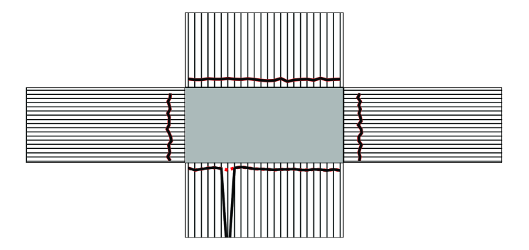
Figure 12: Projected energy deposits of a “single diode” (SD) event.

In view of the projective read out of the VLQ calorimeter, the removal of SD channels is a straight-forward task. Both the horizontal and the vertical scintillator strips are read out at either end. Thus there are two independent energy measurements of each projection, and one can compare the two signal amplitudes from the two ends of a scintillator bar. If the energy in one channel is significantly larger than that in the corresponding opposite one, the channel is treated as a single diode one, and its energy is set to zero.

However, the situation is generally a bit more complicated because a “single diode” and a “real”, i.e. scintillator light induced, event might overlap. Therefore the two neighbouring channels of the suspected SD channel are checked if their amplitudes exceed a certain level above noise. If this is not the case, the central channel is treated as an SD channel and its energy is reset to zero. If the amplitudes are well above noise, they are averaged, and the mean value is assigned to the central channel. This procedure cannot be applied, however, if the single diode candidate is close to one of the calorimeter edges. In this case its amplitude is replaced with that of its opposite partner. SD channels are detected in roughly 25 to 30 % of all events, depending on the running conditions.

After the check for and removal of SDCs, a two step cluster construction is performed. The first step aims at finding “pre-clusters” independently in each of the four projections. To recognize a pre-cluster, the prescriptions of simple calculus to find minima and maxima of an analytic function are applied and transposed in order to handle discrete values as those of calorimeter channel amplitudes. The first and second derivatives are approximated as

$$A^{\prime}(i) = \frac{A(i+1)-A(i)}{h}$$ (3)

$$A^{\prime\prime}(i) = \frac{A(i)-2\cdot A(i+1)+A(i+2)}{h^{2}}.$$ (4)

Here, $h=(i+1)-i=1$ represents the distance between adjacent channels. Before calculating the derivatives, a three $\sigma$ noise cut is applied on the individual channels. This reduces the building of noise clusters due to random fluctuations in the amplitude distribution.

After calculating the derivatives, the channels with minima and maxima in the amplitude distribution are flagged. This is done for each of the four projections independently without using any knowledge from the other projections. The projective readout is then used to cross-check the results by using information from the opposite projection. The numbers of minima and maxima found are compared for each corresponding projection. In the case the numbers do not match, the region in the projection where an extremum was expected, but none was found, is re-examined. This case is quite frequent and is not due to a malfunction of the algorithm, but rather due to scintillator attenuation and cut-off effects. In this step, the noise cut is no longer applied, and the pre-cluster is verified if the channels around the maximum contain at least 40 % of the maximum amplitude. In this case a pre-cluster will be constructed in the projection where previously none was found. To achieve consistency in the number of pre-clusters found in corresponding projections is important because in the final clustering procedure the pre-clusters are combined to form final clusters. In order to verify a cluster, all four projections must match and are needed to reconstruct both x- and y- coordinates.

The situation is somewhat more complicated if two or more particles enter the calorimeter volume. In the case of two clusters (the rare case of three or more clusters can be neglected), there are two possible configurations: The clusters are aligned in either $x-$ or $y-$ direction, or they are distinct. In both cases a pre-cluster construction algorithm is applied analogous to the one - cluster case, with a few assumptions in order to define a cluster separation criterion [15], so that channel energies can be properly assigned to clusters.

As soon as pre-clusters are identified and their energies determined, the energy-weighted coordinates of pre-cluster cells in all four projections are used to calculate the coordinates of the cluster centre of gravity. Following experience with the large backward calorimeter SpaCal [2], a logarithmic weighting procedure is applied. The individual weights of contributing channels $i$ are determined as

$$w_{i}=\max(0,W_{0}+\ln(E_{i}/\sum_{i}E_{i})),$$ (5)

so that the coordinates of the cluster centre of gravity become

$$x_{log}=\frac{\sum_{i}x_{i}w_{i}}{\sum_{i}w_{i}}.$$ (6)

$W_{0}$ is a dimensionless cut-off parameter based on assumptions on the the shower profile [9]. Introducing $W_{0}$ has the effect that only channels above a certain threshold are included in the calculation of the shower centre of gravity. Finally, the cluster radius is calculated as

$$R_{cluster}=\frac{\sum_{i}^{N}E_{i}\cdot\sqrt{(x_{cl}-x_{i})^{2}}}{E_{cl}}$$ (7)

where N is the number of channels associated with the clusters, $x_{cl}$ the cluster center of gravity, and $E_{cl}$ the cluster energy.

After reconstructing the pre-clusters in the four projections, the final (full) cluster properties are determined by adding the pre-cluster energies and averaging the coordinates of the pre-cluster centres.

In case of more than one cluster per projection the situation is more difficult, as illustrated in figure 13:

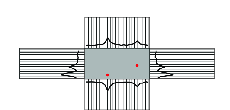
Figure 13: Projected views of a two-cluster event.

Two particles hitting the calorimeter lead to eight pre-clusters from which four clusters can be reconstructed so that there is no unique solution. If however the two incident particles deposit clearly different amounts of energy in the calorimeter, combining the low energy pre-clusters versus the high energy ones allows a non-ambiguous solution. This method will of course fail if the particles have similar energies. In this case no unique solution is possible, and the decision needs to be left over to the VLQ track detector [6].

4 The Calibration Concept

4.1 Test Beam Calibration

Both VLQ calorimeter modules were tested in an electron test beam at the Deutsches Elektronen - Synchrotron DESY in Hamburg. The beam, supplied by the DESY synchrotron, had energies adjustable between 1 and 6 GeV.

In the test setup, the VLQ module to be investigated was fixed at the moving mechanism constructed for operation in H1. As this device supplies only vertical movement, horizontal displacements were performed on a support table driven by a step motor. The vertical and horizontal displacement steps were 5 mm each, corresponding to the scintillator strip width.

The distance between beam collimator and calorimeter module was 5.70 m. The position of the beam in a vertical plane in front of the calorimeter was defined with the help of a silicon tracker telescope. The telescope consisted of two densely packed bundles, each equipped with four Si strip detector planes. The strip orientations were y - x - y - x - x - y - x - y. Each plane contained 384 Si strips of 50 $\mu$m width. The distance between the layers inside one bundle was 10 mm, the two bundles were 17 cm apart from each other. The cross section covered by the telescope was 2 x 2 cm². The Si - telecope was read out sequentially by a 6 - bit CAMAC ADC. It was sandwiched between two scintillation counters which, in coincidence with the telescope signals, provided a trigger pulse. The read-out chain for the VLQ calorimeter modules was identical to that one used in H1 with the exception that the synchronization between test beam generated events and the HERA clock which controlls the readout had to be imposed artificially [9].

Fig. 14 shows a test beam event as a fourfold projection of the energy deposition in the calorimeter. Each of the four histograms displays the (pedestal corrected) contents of the corresponding ADC channels. To determine the shower energy, the entries of the ADC channels of all four histograms have to be summed up.

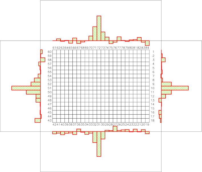
Figure 14: Energy deposit of a 6 GeV electron in the VLQ calorimeter, recorded in a test beam.

In an ideal homogeneous sampling calorimeter of infinite depth, the output signal is proportional to the incident and completely absorbed energy. The proportionality factor which converts ADC counts into energy is called calibration constant.

A real calorimeter is neither perfectly homogeneous nor infinitely deep. The response will depend on the impact position of the primary particle which, together with unavoidable leakage effects, deteriorates the energy (and spatial) resolution. Calibration has therefore a twofold purpose: In a first step, the response of different channels to identical energies must be equalized (“intercalibration”), and in the second step the conversion factor to obtain absolute energies must be determined.

Intercalibration is performed through two independent spatial scans, one along the horizontal side of the calorimeter module, and one along the vertical one. Channel-to-channel responses vary due to inhomogeneities which are mainly caused by imperfect light connections. After a first go-through, the individual single channel responses can be pre-equalized by appropriate weights. In the subsequent step, the spread of output signals will be reduced but still be present, mainly due to light cross talk at the WLS - photodiode connections. Therefore the procedure is repeated until a convergence criterion is fulfilled. In the end, after application of the overall calibration constant to convert Volts into GeV, the individual calibration factors determined for one module have a mean close to one and an r.m.s. of about 10 %, see Fig. 15.

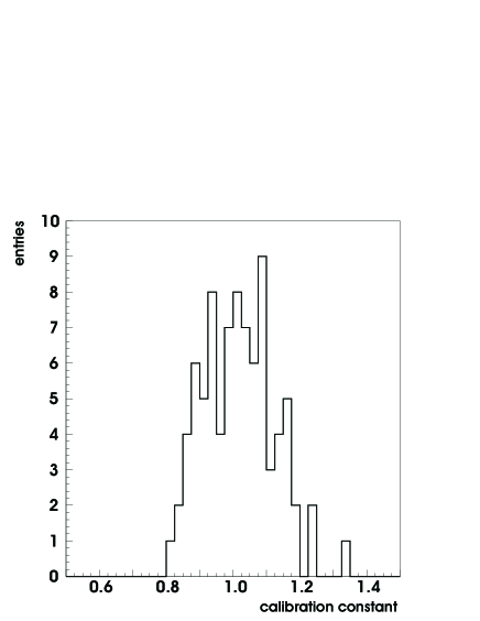
Figure 15: Distribution of calibration factors from test beam measurements.

As mentioned above, the scintillator strips of the VLQ calorimeter show an absorption length much smaller than the corresponding bulk material. This affects the energy reconstruction and requires correction. The light attenuation process was quantified through a test series where the beam impact was varied along a horizontal (vertical) layer of strips, and the corresponding vertical (horizontal) WLS array was read out. The results are shown in Fig. 16 a and b, and where the ADC signal height is plotted as a function of the number of the vertical (a) and horizontal (b) strip hit.

Apparently, the extinction curve shows two components and can be fit, up to the penultimate point, by the sum of two exponentials:

$$F(d)=C_{1}~{}\exp(-\lambda_{1}~{}d)+C_{2}~{}\exp(-\lambda_{2}~{}d),$$

where $d$ denotes the horizontal or vertical distance between beam impact point and light connection, respectively. The reduced light yield from the last strip hit is due to shower particle losses at the calorimeter edge. The enhanced light yield close to the connection scintillator - WLS is caused by its geometry which allows for a wider emission angle at this junction. For the extinction parameters, the fit delivers the results $\lambda_{1,hor}=(0.0128\pm 0.0008)$ cm^-1, $\lambda_{2,hor}=(1.8\pm 0.2)$ cm^-1, $\lambda_{1,vert}=(0.012\pm 0.002)$ cm^-1, and $\lambda_{2,vert}=(2.0\pm 0.2)$ cm^-1.

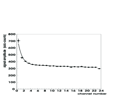
Figure 16: Light attenuation as a function of the scintillator strip hit: a) vertical, b) horizontal strips.

The light extinction is corrected for when applying the final calibration constants.

After an energy scan, the linearity behaviour of the calorimeter can be studied in the available energy range from 1 to 6 GeV. The result is displayed in Fig. 17 which shows the relative deviation from linearity. Deviations are below 1 % and consistent with the simulation results (cf. Fig. 4).

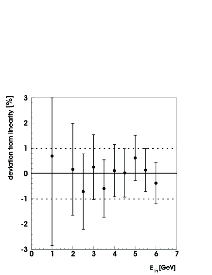
Figure 17: Relative deviations from calorimeter linearity, from test beam measurements in the energy range from 1 to 6 GeV.

An additional result of the energy scan is the energy resolution, which, parametrized as in section 2.1, reads

$$\frac{\sigma(E)}{E}=\sqrt{\left(\frac{(19\pm 6)\%}{\sqrt{E/\text{GeV}}}\right)^{2}\oplus((6.5\pm 3)\%)^{2}\oplus\left(\frac{(23.4\pm 0.9)~{}\%}{E/\text{GeV}}\right)^{2}}.$$ (8)

This is marginally consistent with the simulation result of eq. 2; differences are due to the limited (low) energy range covered by the test beam and its impurities, e.g. due to secondary scattering processes, which tend to distort the energy measurements [9].

The reconstruction of cluster spatial coordinates is also based on the energy measurement: The shower centre of gravity in either projection is expressed as energy weighted mean of scintillator strip coordinates which by construction have a digitization of 5 mm. For consistency, the same five channels are used for spatial reconstruction as for shower energy reconstruction.

The spatial resolution of the calorimeter is determined by comparing the reconstructed beam impact position (according to the procedure described above) and the impact position defined with the help of the silicon tracker matrix whose resolution is roughly 0.1 mm. The result for a beam energy of 4 GeV, for either calorimeter projection, is about 1 mm. The resolution for the horizontal (x -) coordinate is shown in Fig. 18. When parametrizing the spatial resolution as a function of energy, a fit of the form

$$\sigma(x)=\frac{P_{1}[\text{mm}]}{\sqrt{E/\text{GeV}}},$$

yields $P_{1}=(2.06\pm 0.02)$ mm. This implies a resolution of better than one millimeter for energies above 4 GeV.

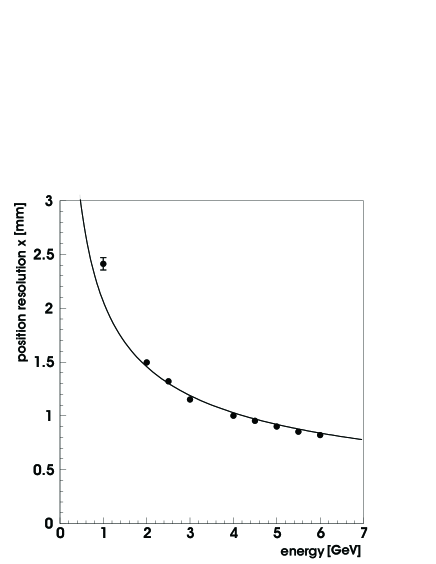
Figure 18: Calorimeter spatial resolution, x - coordinate.

The projective read-out structure of the calorimeter finally allows for a direct sampling of the lateral shower profile. This is performed by measuring a large number of showers in the central area of a calorimeter module, at an energy of 4 GeV. In a large number of measurements, noise and statistical fluctuations in the shower profile cancel. The bin size is given by the resolution (about 1 mm). In Fig. 19 all shower profiles are plotted versus the radial distance from the shower axis such that each shower centre is shifted to R = 0. One recognizes a two - component structure of the profile which can be parametrized as the sum of two exponentials. A fit to the distribution of Fig. 19 yields, for the two parameters for the “fast” and “slow” lateral damping, the values $(2.2\pm 0.1)$ cm^-1 and $(0.77\pm 0.05)$ cm^-1.

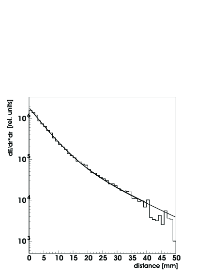
Figure 19: A transverse shower profile, i.e. energy deposition as a function of distance from the shower axis, at an energy of 4 GeV as determined in the test beam.

Integrating the exponential profile function with these parameters yields a Molière radius of 1.5 cm which is slightly larger than the value predicted by the simulation (1.25 cm, see section 2.1). The difference is explained by optical cross talk between neighbouring scintillator and read-out channels which leads to an apparent shower broadening, and which was not taken into account in the simulation.

The following Table 2 gives an overview over the most important parameters quantifying the VLQ calorimeter’s performance in the test beams.

Energy resolution, sampling term	(19 $\pm$ 6) %
Energy resolution, constant term	(6.5 $\pm$ 3.0) %
Energy resolution, noise term	(23 $\pm$ 1) %
Deviation from linearity	$<$ 1 %
Horizontal (vertical) spatial resolution	$<$ 1 mm for E $>$ 4 GeV
Molière Radius	1.5 cm

Table 2: Measured VLQ calorimeter performance parameters.

4.2 Normal Calibration Using the “Kinematical Peak”

In order to calibrate the VLQ calorimeter during the standard experimental data taking phase and at high energies, the observation of the “kinematical peak” in electron - proton scattering is exploited: In the energy spectrum of electrons scattered off protons with moderate $Q^{2}$, a peak appears at the position of the incident electron beam energy. The response of a calorimeter can be adjusted accordingly.

The calibration proceeds in several steps: After selecting the kinematical peak events, a channel-to-channel intercalibration is performed in order to homogenize channel responses. This is followed by adjusting the absolute energy scale in terms of position dependent calibration factors.

4.2.1 Event Selection and Channel-to-Channel Intercalibration

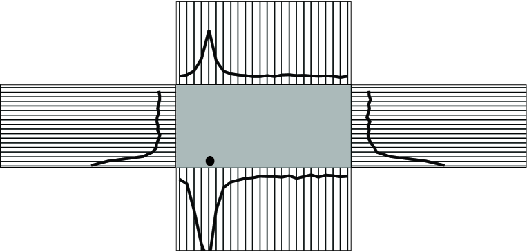
Figure 20: Projected views of a “Kinematical Peak” event.

Events to be used for the kinematical peak calibration must fulfil the following selection criteria: The electron must deposit an energy above the highest trigger threshold in one of the calorimeter modules; the value of the “inelasticity” $y$ reconstructed following the prescription by Jacquet and Blondel [16] which indicates hadronic energy deposition in the central calorimeter must obey $y_{JB}\leq 0.04$; as at HERA the electron beam energy is $27.56\,\text{GeV}$, only clusters with energies $E_{cl}\geq 20.0\,\text{GeV}$ are accepted. A requirement of the reconstruction software is that exactly one cluster and no SD channel was found, or at least no SD channel which is connected to the cluster.

The aim of the channel-to-channel intercalibration is to ensure that equal energy depositions result in equal responses of all channels. Variations in the channel energy responses can have different sources, the most important ones are due to optical and electronical cross talk. The optical cross talk is due to light emission into neighbouring photodiodes, caused by overlapping light cones in the thin glass pane between wavelength shifters and photodiode surfaces.

The channel-to-channel calibration is a two step procedure whose principle has been sketched in Section 4.1 . The algorithm used for the normal calibration is briefly described below:

In a first step the signal of the channel with the maximum energy deposition is filled into a histogram associated to that specific channel, and the mean for each channel is determined. In order to calculate calibration factors, a reference value is needed which in this case is the “mean of (the above defined) means”, averaged over all channels belonging to one wavelength shifter array. This procedure is expressed in the following equation:

$$M^{(1)}=\frac{\sum_{i,N_{i}\geq N_{limit}}m_{i}^{(1)}}{n^{(1)}.}$$ (9)

Here, $n^{(1)}$ is the number of channels entering the average after the first iteration, and $m_{i}^{(1)}$ is the mean value of the histogram which contains the measured energies of channel $i$.

$M^{(1)}$ is the global mean in an given wavelength shifter array for the first iteration. The effect of the calibration is such that after applying the first iteration calibration constants

$$f_{i}^{(1)}=\frac{M^{(1)}}{m_{i}^{(1)}.}$$ (10)

the mean energy in any channel is shifted to the global mean. This procedure is then repeated until the change in the mean energy of any channel with respect to the previous iteration is smaller than $0.5$%.

The second intercalibration iteration has the purpose to correct for inhomogeneities caused by optical cross talk between adjacent wavelength shifter bars, which is of the order of $10$% [9]. It is performed after the calibration factors of the first step have been applied. The procedure is identical to the previous one with the exception that this time the “maximum channel” energy plus two “left” and two “right” neighbours are summed up and filled into the histogram. In this way, with the iterations carried out as in step one, the “light sharing” between neighbouring channels due to optical cross talk is taken into account. The distribution of the calibration factors resulting from this procedure, for the first of the two calorimeter modules, is shown in Fig. 21. The distribution for the second module is similar [15]. The channels with calibration factors close to 2 suffered from a broken light connection at one end.

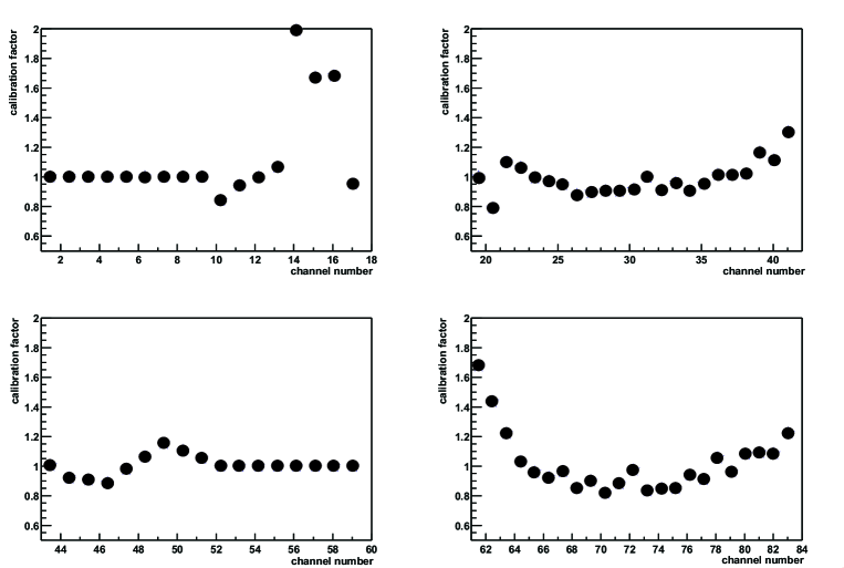
Figure 21: Channel-to-channel calibration factors.

4.2.2 Determination of the Absolute Energy Scale and Impact Position Dependent Calibration

The calibration has to result in correction factors which ensure that the energy response for a given particle energy is the same for all possible impact positions. This was partly done in the intercalibration steps described above, but due to the light collection effects mentioned and described in Section 2.3, the regions close to the calorimeter edges are not covered yet. Therefore in the final step of the calibration procedure the absolute energy scale in terms of position dependent calibration factors is determined.

This correction becomes especially important for impact positions close to the calorimeter edges where parts of the deposited energy leak out of the active calorimeter volume into transverse direction, and where scintillator light yield effects play an important role [12]. After homogenizing the individual channel responses, the absolute energy scale and the position dependend calibration factors are determined.

To homogenize the detector response, the detector surface is subdivided into segments of $5\times 5\,\text{mm}^{2}$ in the central region, and $1\times 1\,\text{mm}^{2}$ bins close to the edges where the response depends strongly on the distance from the calorimeter edge. The mean energy $\epsilon_{ij}$, averaged over all events reconstructed in that bin, is calculated. The calibration factor $A_{i,j}$ is calculated by normalizing the mean energy in the bin $ij$ to the known HERA kinematical peak energy of $27.56\,\text{GeV}$:

$$A_{i,j}=\frac{27.56\,\text{GeV}}{\epsilon_{i,j}}.$$ (11)

The calibration constants have been determined from H1 data for the channels providing sufficient statistics. The mean value of the constants is 1.125 with an r.m.s. spread of 0.040 .

4.2.3 Energy Resolution after Calibration

For the kinematical peak calibration two data samples were used, namely from April 1999 and from September - October 1999. The energy resolution after calibration, as a function of energy and from both test beam and kinematical peak data, is displayed in Fig. 22. Using the available data at lower and high energies, an energy resolution parametrized as

$$\frac{\sigma_{E}}{E}=\sqrt{\bigg{(}\frac{(9.16\pm 4.31)\%}{\sqrt{E/\text{GeV}}}\bigg{)}^{2}+\bigg{(}(6.04\pm 0.22)\%\bigg{)}^{2}+\bigg{(}\frac{(31.94\pm 3.48)\%}{E/\text{GeV}}\bigg{)}^{2}}$$ (12)

is derived. The individual contributions from sampling term, constant term, and noise term are indicated in the figure.

When compared to the parametrization of the resolution curve obtained from test beam data (Eq. 8), a significant increase of the noise term is observed. This is a consequence of the electronic environment present in the H1 experimental hall which is very much different from the situation in the test beam area. The additional point taken at the HERA electron beam energy constrains the fit at high energy so that the constant term can be determined with high accuracy. No such measurement was available in the test beam. The sampling term is consistent with both that obtained from a simulation (Eq. 2) and from the low energy test beam data.

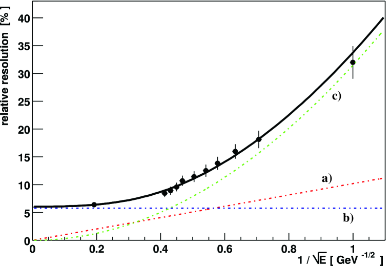
Figure 22: VLQ energy resolution as a function of energy. The dash - dotted lines indicate the influence of the contributing terms: a) “sampling term”, b) “constant term”, and c) “noise term”.

5 Performance at HERA

During its two years of operation in the H1 experiment at HERA, the main purpose of the VLQ spectrometer was the detection of high energy electrons and photons in the context of structure function measurements [17] and meson spectroscopy. The performance of the calorimeter is demonstrated best with purely electromagnetic interactions where no other H1 detector component is involved, e.g. with wide angle bremsstrahlung events, also called “QED Compton (QED-C)” events [18], i.e.

$$e^{-}~{}p~{}\rightarrow~{}p~{}e^{-}~{}\gamma.$$

A striking feature of QEDC events is, due to the generally very small four-momentum transfer to the target proton, the coplanarity of the final state electron and photon: In the transverse detector plane (“r - $\phi$ - plane”) photon and electron momentum vector components are back - to - back. In addition, the sum of photon and final state electron energy must equal the initial electron beam energy.

The VLQ calorimeter is ideally suited to test these properties (or, to profit from them because they can be used for calibration and alignment purposes as described in [18]). The performance of the calorimeter is demonstrated in Figs. 23 and 24, taken from [18]. Fig. 23 shows the sum of final state electron and photon energies, together with the result of a simulation, and Fig. 24 shows the azimuth angular difference, shifted by $180^{\circ}$, of photon and electron impact points, again compared to a simulation. Apparently, the calorimeter behaved as expected.

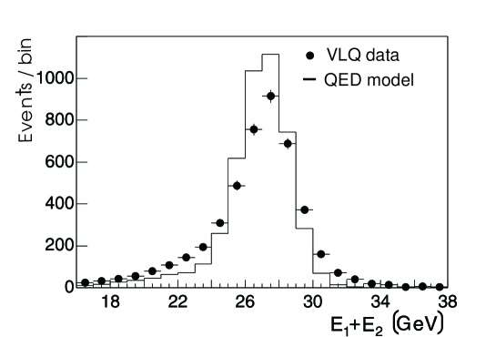
Figure 23: Sum of photon- and electron energies for QED - Compton events measured in the VLQ calorimeter. Comparison of data and QED simulation.

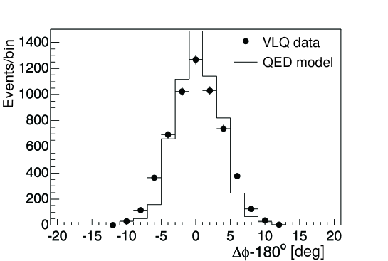
Figure 24: Azimuth angular difference of photon and electron impact points in the VLQ calorimeter, for QED Compton events. Comparison of data and QED simulation.

In the context of an analysis searching for single $\pi^{0}$’s produced in the H1 backward region [5], two - photon pairs were collected and investigated for a signal, where either both photons had to be detected in the VLQ calorimeter, or one photon in the VLQ and the other one in the SpaCal backward calorimeter. The low cross section, in combination with special kinematic restrictions, did not leave a sizeable signal for the VLQ - VLQ case alone.

A clear $\pi^{0}$ signal was observed, however, if the combination VLQ - SpaCal is added, see Fig. 25 where a fit of a Gaussian function to the $\pi^{0}$ peak plus a polynomial for the background is superimposed. The $\pi^{0}$ peak is shifted towards a mass larger than the PDG value, and appears broader than expected for both SpaCal and VLQ mass resolutions [19]. There are several reasons responsible for these effects: First, the position of the actual interaction vertex is not known because there are no charged particle tracks in these events, and four-momenta have to be reconstructed using the nominal vertex position. Second, both the SpaCal and VLQ calibrations were performed with the help of the “Kinematical Peak”, i.e. with electrons of an energy close to the incident electron beam energy (see Section 4.2) while photons from $\pi^{0}$ decays have much smaller energies. Third, no dedicated intercalibration was performed between the SpaCal and VLQ calorimeters. In spite of these limitations, the capability of the VLQ to contribute to the reconstruction of $\pi^{0}$’s from their decays to two photons is convincingly demonstrated.

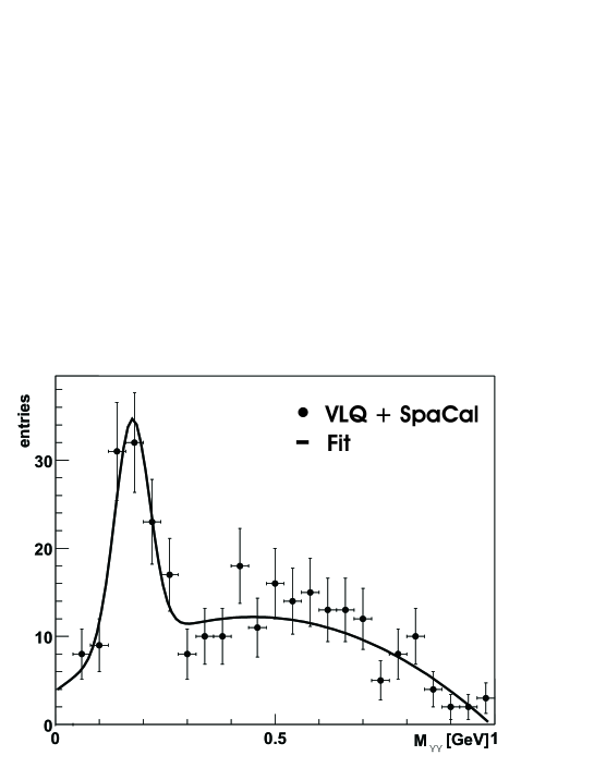
Figure 25: Two - photon invariant mass distributions from photoproduction events where one photon is measured in the VLQ, and one in the SpaCal.

6 Conclusions

The Very Low $\text{Q}^{2}$ calorimeter of H1, a highly compact device designed to measure high energetic electrons and photons in the electron beam downstream region, was succcessfully operated in the 1999 and 2000 data taking periods. The performance in the experiment was very close to that expected from design and simulations. The VLQ calorimeter contributed significantly to measurements of the proton structure function $F_{2}$ in phase space regions previously unaccessible for H1, and opened a new kinematical regime for the spectroscopy of mesons decaying to purely photonic final states.

References

- [1] H1 Collaboration, I. Abt et al., Nucl. Instr. and Meth. A 386 (1997) 310 and 348.
-
[2]
H1 SpaCal Group, T. Nicholls et al.,
Nucl. Instrum. Methods A374 (1996) 149;
H1 SpaCal Group, R.D. Appuhn et al., Nucl. Instrum. Methods A382 (1996) 395;
H1 SpaCal Group, R.D. Appuhn et al., Nucl. Instrum. Methods A386 (1997) 397. - [3] The H1 Collaboration, “Technical Proposal to Build a Special Spectrometer Covering Very Small Momentum Transfers” TP-VLQ, May 8, 1996; revised version may 31, 1996.
-
[4]
E. R. Berger, A. Donnachie, H. G. Dosch, W. Kilian,
O. Nachtmann and M. Rüter,
Eur. Phys. J. C 9(1999) 491 - [5] The H1 Collaboration, C. Adloff et al., Phys. Lett. B554 (2002) 35.
- [6] Stephan Hurling, “Der VLQ - Detektor bei H1: Inbetriebnahme, Spurrekonstruktion und Messung der elastisch diffraktiven - Produktion bei kleinem ”, Dr. rer. nat. Dissertation, Hamburg, 2000.
- [7] BICRON Industrial Ceramics Corporation, BC-400 / BC-404 / BC-408 / BC-412 / BC-416 / Data Sheet, 1996.
- [8] R. Brun, R. Hagelberg, M. Hansroul, J. C. Lassalle, “GEANT: Simulation Program for Particle Physics Experiments”. Users’ Guide and Reference Manual, CERN-DD-78-2-REV.
- [9] Achim Stellberger, “Entwicklung und Bau eines kompakten elektromagnetischen Kalorimeters” HD-IHEP-98-04, Dissertation, Heidelberg, 1998.
-
[10]
M. Keller, K. Meier, O. Nix, G. Schmidt, A. Stellberger, J. Stiewe,
Nucl. Instr. Meth.
A 409 (1998) 604. - [11] BICRON Industrial Ceramics Corporation, BC-482A Data Sheet, 1996.
- [12] Günter Schmidt, “Test eines optoelektronischen Kalorimeterauslesesystems” HD-IHEP-97-04, Diploma Thesis, Heidelberg, 1997.
- [13] J. Bán et al., Nucl. Instr. Meth. A372 (1996) 399.
- [14] The H1 Calorimeter Group, Nucl. Instr. Meth. A336 (1993) 460.
- [15] Oliver Nix, “Suche nach odderoninduzierten Beiträgen in exklusiver - Produktion mit dem Detektor H1 bei HERA” HD-KIP-01-05, Dissertation, Heidelberg, 2001.
-
[16]
A. Blondel and F. Jacquet, Proceedings of the Study of
an Facility for Europe,
ed. U. Amaldi, DESY 79/48 (1979) 391. - [17] Carlo Duprel, “Measurement of the Proton Structure Function at Low x and Low with the H1 Detector at HERA”, Dissertation, RWTH Aachen, in preparation.
- [18] Thomas Kluge, “Untersuchung des QED - Bremsstrahlungsprozesses bei kleinen Impulsuebertraegen mit dem H1 - Detektor bei HERA”, Diploma Thesis, RWTH Aachen, 2000.
- [19] Tobias Golling, “Search for Odderon Induced Contributions to Exclusive Photoproduction at Hera”, HD-KIP-01-03, Diploma Thesis, Heidelberg, 2001.