Going forth and back in time :
a fast and parsimonious algorithm for mixed initial/final-value problems

Abstract

We present an efficient and parsimonious algorithm to solve mixed initial/final-value problems. The algorithm optimally limits the memory storage and the computational time requirements : with respect to a simple forward integration, the cost factor is only logarithmic in the number of time-steps. As an example, we discuss the solution of the final-value problem for a Fokker-Planck equation whose drift velocity solves a different initial-value problem – a relevant issue in the context of turbulent scalar transport.

, ,

1 Introduction

In the investigation of dynamical systems, the standard initial-value problem is to compute from the equations of motion the state of the system at a final time $t$, given its initial condition at time $t_{0}$. Sometimes, however, the state of the system might be known at a final time $t$, and one would be interested in evolving the system backward in time to compute its earlier states, back to $t_{0}$. This can in theory be easily accomplished by reversing the direction of the time-integration, thus transforming the final-value problem in an initial-value one. Problems might however appear if the forward evolution is given by a mapping that is not one-to-one, as the previous state can thus become undefined. Even if the time evolution is given by a differential system, the backward evolution becomes unstable if the forward dynamics is dissipative, as is the case in many physical systems, like for instance Navier-Stokes turbulence. The problem stems from the fact that a dissipative system contracts volumes in phase space in the forward direction, and thus expands them in the backward direction and amplifies any small numerical errors, like those caused by roundoff.

Another quite difficult task is to obtain the evolution of a system when part of the variables that specify the state are given at an initial time $t_{0}$ and the remaining ones are given at the final time $t$. We refer to this class of problems as “mixed initial/final-value”. We will be interested in a special subclass of such problems, that can be schematically written as follows

$${\d{\bm{u}}\over\d s} = {\bm{f}}({\bm{u}},s)\,,\qquad\,\;\;\;\;{\bm{u}}(t_{0})\!={\bm{u}}_{0}\;$$ (1)

$${\d{\bm{z}}\over\d s} = {\bm{g}}({\bm{z}},{\bm{u}},s)\,,\qquad\;{\bm{z}}(t)={\bm{z}}_{t}\;,$$ (2)

where ${\bm{u}}$ and ${\bm{z}}$ are vectors in a given space. Far from being an academic oddity, this problem is relevant to many physical situations, among which we will discuss in detail the transport of scalar fields by a dynamically evolving flow. Consider indeed the problem of finding the solution ${\bm{a}}(s)$ of the stochastic differential equation

$${\d{\bm{a}}(s)\over\d s}={\bm{v}}({\bm{a}}(s),s)+\sqrt{2\kappa}\,{\bm{\eta}}(s)\;,$$ (3)

with the final value ${\bm{a}}(t)={\bm{x}}$.

Eq. (3) describes the evolution of a particle transported by the velocity field ${\bm{v}}$ and subject to molecular diffusion with diffusivity $\kappa$, represented here by the zero-mean Gaussian process ${\bm{\eta}}$ with correlations $\langle\eta_{i}(t)\eta_{j}(t^{\prime})\rangle=\delta_{ij}\delta(t-t^{\prime})$. The velocity field ${\bm{v}}$ at any time $s$ has to be obtained from some dynamical law (e.g. the Navier-Stokes equations) and from its initial value at $s=t_{0}$. It is easy to recognize that ${\bm{v}}$ plays the role of the variable ${\bm{u}}$ in Eqs. (1-2) whereas ${\bm{a}}$ has to be identified with ${\bm{z}}$. An equivalent description may be given in terms of the transition probability $P({\bm{y}},s|{\bm{x}},t)$ – i.e. the probability that a particle is in ${\bm{y}}$ at time $s$ given that it will be in ${\bm{x}}$ at time $t$. The propagator evolution is ruled by the well known Kolmogorov equation [1, 2]

$$-\partial_{s}P({\bm{y}},s|{\bm{x}},t)-{\bm{\nabla}}_{\!y}\cdot[{\bm{v}}({\bm{y}},s)P({\bm{y}},s|{\bm{x}},t)]=\kappa\,\nabla^{2}_{y}P({\bm{y}},s|{\bm{x}},t)\;,$$ (4)

where the final condition is set : $P({\bm{y}},t|{\bm{x}},t)=\delta({\bm{x}}-{\bm{y}})$. In the latter case, it is $P$ that has to be interpreted as ${\bm{z}}$ in (2).

In this article, we propose a fast and memory-sparing algorithm to solve the problem (1-2) or to allow one to go back through the time evolution if the dynamics is unstable or non-invertible. In Sec. 2 we describe in detail the algorithm, comparing it to more naive and less efficient strategies. In Sec. 3 we present an application to the problem of front generation in passive scalar turbulence (see e.g. [3, 4]).

2 Backward Algorithm

The obvious difficulty with Eqs. (1–2) resides in the fact that, since the initial conditions of ${\bm{u}}$ and ${\bm{z}}$ are set at different times, they cannot be evolved in parallel. Also, the time evolution of ${\bm{u}}(s)$ might be non-invertible or unstable in the backward time direction. The whole history of ${\bm{u}}(s)$ in the interval $[t_{0},t]$ is thus needed to integrate ${\bm{z}}(s)$ from time $t$ back to time $t_{0}$.

Before presenting our own algorithm, we wish to discuss some naive strategies to expose their shortcomings and advantages, and introduce notations. In the following, we will assume the whole time interval $[t_{0},t]$ to be discretized in $N$ identical time steps, small enough to ensure accurate integration of Eqs. (1–2). The states ${\bm{u}}(s)$, ${\bm{z}}(s)$ thus have to be computed at the $N+1$ times $t_{0},\ldots,t_{j}\equiv t_{0}+(t-t_{0})j/N,\ldots,t_{N}\equiv t$. In our applications, the states ${\bm{u}}(s)$ and ${\bm{z}}(s)$ will be $d$-dimensional vector fields, numerically resolved with $\mathcal{L}^{d}$ collocation points, and therefore have a size $O(d\,\mathcal{L}^{d})$, typically very large, that will be taken as unit of measure when describing the storage requirements $\mathcal{S}(N)$ of the different algorithms. The CPU time cost $\mathcal{T}(N)$ will refer only to (forward) integrations of ${\bm{u}}$ and will be expressed in terms of the time to perform a single forward integration step. We will also give examples of memory use and CPU time for $d=2$, $\mathcal{L}=1024$ and $N=2^{14}$, which are typical values of moderately resolved direct numerical simulations in computational fluid dynamics, requiring 16 MB of memory to store a single state array.

The most obvious and simple strategy is the following :

A1. integrate forward Eq. (1) from $t_{0}$ to $t_{N}$ and store ${\bm{u}}(s)$ at all time steps $t_{0}\ldots t_{N}$ ;

A2. integrate backward Eq. (2) from $t_{N}$ back to $t_{0}$.

The number of integration steps needed by this procedure is $\mathcal{T}(N)=N$, while the memory storage cost is a frightening $\mathcal{S}(N)=N$. As soon as the dimensionality of the space or the number of collocation points increase, this approach becomes rapidly unfeasible. Taking our typical fluid dynamics value, one would need 256 GB of memory, which is clearly irrealistic.

A different strategy that minimizes the memory requirements is :

B1. set $n\leftarrow N$ and store the initial condition ${\bm{u}}_{0}$ ;

B2. integrate forward Eq. (1) from $t_{0}$ to $t_{n}$ ;

B3. integrate backward Eq. (2) from $t_{n}$ to $t_{n-1}$, update $n\leftarrow n-1$, and go back to step B2 if $n\geq 0$.

While this method is very advantageous in memory $\mathcal{S}(N)=1$, it is prohibitively expensive because of the large number of iterations needed : $\mathcal{T}(N)=N(N+1)/2$. With the previously given numerical parameters, one needs a daunting increase by a factor $8200$ in CPU time with respect to algorithm A.

To improve algorithm B, one can think of using more memory and a simple generalization goes as follows :

C1. integrate forward Eq. (1) from $t_{0}$ to $t_{N}$ and store the states ${\bm{u}}(s)$ at the $M$ equidistant times $\tau_{k}=t_{Nk/M},\;k=0,\ldots,M-1$ (we assume here $N$ to be a multiple of $M$ for convenience) ;

C2. apply algorithm B successively in each segment $[\tau_{k},\tau_{k+1}]$.

The number of operations is $\mathcal{T}(N)=N(N+M)/(2M)$ remains however prohibitive unless we raise $M$ to be $O(N)$. Now, since the memory storage is $\mathcal{S}(N)=M$, $M$ cannot be made too large as well. Again refering to the numerical parameters given above, we have that for $M=16$ the storage requirement is reasonably low (256 MB) yet the time factor with respect to algorithm A is a still discouraging 512.

A further possibility which helps reducing the number of iterations and is almost reasonable for the memory storage needs is :

D1. integrate forward Eq. (1) from $t_{0}$ to $t_{N}$ and store $M$ states ${\bm{u}}(s)$ at times $\tau_{k}=t_{Nk/M},\;k=0,\ldots,M-1$. Set $k\leftarrow M-1$ ;

D2. integrate forward Eq. (1) from $t_{Nk/M}$ to $t_{N(k+1)/M}$, using the stored state at $\tau_{k}$ as initial condition and saving the states ${\bm{u}}(s)$ at all time steps in a further set of $N/M$ storage locations ;

D3. integrate backward Eq. (2) from $t_{N(k+1)/M}$ to $t_{Nk/M}$ using the $N/M$ saved ${\bm{u}}(s)$, update $k\leftarrow k-1$ and go back to step D2 if $k\geq 0$.

This procedure needs a reasonable total number of time steps $\mathcal{T}(N)=N+(N-M)(M-1)/M$, that is $\mathcal{T}(N)\approx 2N$ when $N\gg M\gg 1$, and is thus asymptotically linear in $N$, provided we have enough memory. The storage requirement is indeed rather large $\mathcal{S}(N)=M+N/M$ and is minimized for a fixed $N$ by taking $M=\sqrt{N}$. With our typical parameters, we would have to take $M=128$ and store 256 fields, amounting to roughly 4 GB, still too large for typical workstations.

Algorithm D is still too greedy in memory, but it gives the idea of dividing the problem into smaller subproblems that have a much smaller running time, and that be combined later to give the full solution. If we push this idea further, we can build a recursive algorithm that integrates backward from $t_{N}$ to $t_{0}$ by integrating forward from $t_{0}$ to $t_{N/2}$, and using the states at $t_{0}$ and $t_{N/2}$ to call itself successively in the intervals $[t_{N},t_{N/2}]$ and $[t_{N/2},t_{0}]$. We have chosen here the subdivision base (the equivalent of $M$ in the previous algorithm) to be 2, because it gives the simplest and one of the most efficient algorithms, but other bases could be used to slightly reduce the number of integration steps, at the price of using more storage. Of course, recursion can be eliminated and it is in its non-recursive form that we will describe our procedure. To do that, we will need a stack, that is a list of states to which we can add (push/save) a new item or remove (pull/delete) the last stored item. A stack can always be implemented as an array in programming languages that do not have it as a built-in type. We will also use the index $[{\rm top}]$ to refer to the (last pushed) element on top of the stack. Our algorithm is then very easy to state :

R1. set the desired time index $n\leftarrow N$ and push the initial condition ${\bm{u}}_{0}$ on the stack ;

R2. if the state on top of the stack does not correspond to the index $n$, set $j\leftarrow(j_{[{\rm top}]}+n+1)/2$ to the upper midpoint of the interval, integrate forward ${\bm{u}}_{[{\rm top}]}$ from $t_{[{\rm top}]}$ to $t_{j}$, push the state ${\bm{u}}_{j}$ on the stack and go back to step R2 ;

R3. pull the state ${\bm{u}}_{[{\rm top}]}\equiv{\bm{u}}_{n}$ from the stack, use it to integrate backward Eq. (2) from $t_{n}$ to $t_{n-1}$, set $n\leftarrow n-1$, and go back to step R2 if $n\geq 0$.

Time	Stack	Steps	Total steps
$s=t_{20}$	${\bm{u}}_{0}$ ${\bm{u}}_{10}$ ${\bm{u}}_{15}$ ${\bm{u}}_{18}$ ${\bm{u}}_{19}$ ${\bm{u}}_{20}$	20	20
$s=t_{19}$	${\bm{u}}_{0}$ ${\bm{u}}_{10}$ ${\bm{u}}_{15}$ ${\bm{u}}_{18}$ ${\bm{u}}_{19}$	0	20
$s=t_{18}$	${\bm{u}}_{0}$ ${\bm{u}}_{10}$ ${\bm{u}}_{15}$ ${\bm{u}}_{18}$	0	20
$s=t_{17}$	${\bm{u}}_{0}$ ${\bm{u}}_{10}$ ${\bm{u}}_{15}$ ${\bm{u}}_{16}$ ${\bm{u}}_{17}$	2	22
$s=t_{16}$	${\bm{u}}_{0}$ ${\bm{u}}_{10}$ ${\bm{u}}_{15}$ ${\bm{u}}_{16}$	0	22
$s=t_{15}$	${\bm{u}}_{0}$ ${\bm{u}}_{10}$ ${\bm{u}}_{15}$	0	22
$s=t_{14}$	${\bm{u}}_{0}$ ${\bm{u}}_{10}$ ${\bm{u}}_{12}$ ${\bm{u}}_{13}$ ${\bm{u}}_{14}$	4	26
$s=t_{13}$	${\bm{u}}_{0}$ ${\bm{u}}_{10}$ ${\bm{u}}_{12}$ ${\bm{u}}_{13}$	0	26
$s=t_{12}$	${\bm{u}}_{0}$ ${\bm{u}}_{10}$ ${\bm{u}}_{12}$	0	26
$s=t_{11}$	${\bm{u}}_{0}$ ${\bm{u}}_{10}$ ${\bm{u}}_{11}$	1	27
$s=t_{10}$	${\bm{u}}_{0}$ ${\bm{u}}_{10}$	0	27
$s=t_{9}$	${\bm{u}}_{0}$ ${\bm{u}}_{5}$ ${\bm{u}}_{7}$ ${\bm{u}}_{8}$ ${\bm{u}}_{9}$	9	36
$s=t_{8}$	${\bm{u}}_{0}$ ${\bm{u}}_{5}$ ${\bm{u}}_{7}$ ${\bm{u}}_{8}$	0	36
$s=t_{7}$	${\bm{u}}_{0}$ ${\bm{u}}_{5}$ ${\bm{u}}_{7}$	0	36
$s=t_{6}$	${\bm{u}}_{0}$ ${\bm{u}}_{5}$ ${\bm{u}}_{6}$	1	37
$s=t_{5}$	${\bm{u}}_{0}$ ${\bm{u}}_{5}$	0	37
$s=t_{4}$	${\bm{u}}_{0}$ ${\bm{u}}_{2}$ ${\bm{u}}_{3}$ ${\bm{u}}_{4}$	4	41
$s=t_{3}$	${\bm{u}}_{0}$ ${\bm{u}}_{2}$ ${\bm{u}}_{3}$	0	41
$s=t_{2}$	${\bm{u}}_{0}$ ${\bm{u}}_{2}$	0	41
$s=t_{1}$	${\bm{u}}_{0}$ ${\bm{u}}_{1}$	1	42
$s=t_{0}$	${\bm{u}}_{0}$	0	42

Figure 1: Algorithm R in action for $N=20$. The state of the stack is shown for every time $t_{j}$ at the beginning of label R3, where the state ${\bm{u}}(t_{j})$ becomes available on top of the stack. Steps is the number of forward integration steps needed for this particular time, while Total steps is the number of forward steps since the final time $t_{20}$ to the current time.

To understand better the behavior of algorithm R, the easiest is to show an example of how it works in a simple case for a small value of $N$. Fig. 1 does this for $N=20$, showing the stack movements at every time step. Even for such a small value of $N$, algorithm R needs 3.5 times less memory and is only 2.1 times slower than algorithm A, while it is 5 times faster than algorithm B.

It is obvious that our algorithm needs a very small amount of storage $\mathcal{S}(N)=1+\lceil\log_{2}(N)\rceil$, that is only 15 fields or 240 MB for our typical example with $N=2^{14}$. The computing time is also very reasonable : the computing time $\mathcal{T}(N)$ obeys the recursions $\mathcal{T}(N)=2\,\mathcal{T}(N/2)+N/2-1$ if $N$ is even and $\mathcal{T}(N)=2\,\mathcal{T}(\lfloor N/2\rfloor)+\lceil N/2\rceil$ if it is odd. The number of steps thus depends on the precise binary representation of $N$, but is given approximately by $\mathcal{T}(N)\approx N\lceil\log_{2}(N+1)\rceil/2+1$ (equality being achieved if $N$ is a power of 2), that is a cost factor that is only logarithmic in the number of time steps. In our same example, we find that we will need 7 times more integration steps than the brute force algorithm A, but 1100 times less storage, so that the whole stack can be kept in-core during the backward integration.

The algorithm we propose is thus quite efficient in computing time, and very economical in memory, opening the door to the study of the backward evolution of very large multi-dimensional fields. To give an idea of possible applications, one might study the “seed” at $t_{0}$ that gave birth to a particular structure observed at time $t$. As an example, we will discuss in the following section the numerical implementation and an application of this algorithm to scalar transport in turbulent flows.

3 Scalar fields in turbulent flows

The transport of scalar fields, such as temperature, pollutants and chemical or biological species advected by turbulent flows, is a common phenomenon of great importance both in theory and applications [3]. A scalar field, $\theta({\bm{x}},t)$, obeys the advection-diffusion equation

$$\partial_{t}\theta+{\bm{v}}\cdot{\bm{\nabla}}\theta=\kappa\nabla^{2}\,\theta+\phi\;,$$ (5)

where $\kappa$ is the molecular diffusivity, ${\bm{v}}$ is the velocity field, and $\phi$ is the scalar input acting at a characteristic lengthscale $L_{\phi}$. The presence of a scalar source allows for studying stationary properties. Thanks to the linearity of Eq. (5), the problem can be solved in terms of the particle propagator [3, 4]

$$\theta({\bm{x}},t)=\int_{0}^{t}\!\!\d s\int\!\!\d{\bm{y}}\;P({\bm{y}},s|{\bm{x}},t)\,\phi({\bm{y}},s)\;,$$ (6)

as can be directly checked by inserting (6) in (5) and using (4). To make more intuitive the physical content of Eq. (6), we can rewrite it as

$$\theta({\bm{x}},t)=\left\langle\int_{0}^{t}\!\!\d s\;\phi({\bm{a}}(s),s)\right\rangle_{\bm{a}}\;,$$ (7)

where $\langle\ldots\rangle_{\bm{a}}$ denotes the average over particle trajectories obeying (3) with ${\bm{a}}(t)={\bm{x}}$. From (7) one understands that $\theta({\bm{x}},t)$ is built up by the superposition of the input along all trajectories ending at point ${\bm{x}}$ at time $t$.

The velocity field evolves according to the Navier-Stokes equation :

$$\partial_{t}{\bm{v}}+{\bm{v}}\cdot{\bm{\nabla}}{\bm{v}}=-{\bm{\nabla}}p+\nu\nabla^{2}{\bm{v}}+{\bm{f}}\;.$$ (8)

Where the pressure $p$ is fixed by the incompressibility condition (${\bm{\nabla}}\cdot{\bm{v}}=0$), $\nu$ is the kinematic viscosity, and ${\bm{f}}$ the energy input. Notice that $\theta$ does not enter the equation for the velocity field and therefore the scalar is called passive.

In the following we will consider a passive scalar field evolving in a two dimensional turbulent velocity field, and show how the numerical study of particle propagator conveys some information on the dynamical origin of structures in the scalar field.

3.1 Numerical Implementation

We integrate Eqs. (5), (8) and (4) in a doubly periodic box $2\pi\times 2\pi$ with $\mathcal{L}_{x}\times\mathcal{L}_{y}$ grid points (the results here discussed are for $\mathcal{L}_{x}=\mathcal{L}_{y}=1024$) by a standard $2/3$-dealiased pseudo-spectral method [5, 6]. A detailed description of the properties of the velocity field in two-dimensional Navier-Stokes turbulence can be found in [7]. Here we only mention that the velocity field is self-similar with Kolmogorov scaling i.e. $({\bm{v}}({\bm{x}}+{\bm{r}},t)-{\bm{v}}({\bm{x}},t))\cdot{\bm{r}}/r\sim r^{1/3}$. However, the passive scalar increments $\theta({\bm{x}}+{\bm{r}})-\theta({\bm{x}})$ are not self-similar, since large excursions occur with larger and larger probability for increasingly small separations $r$ (see, e.g., [8, 9]).

Time integration of Eqs. (5) and (8) is performed using a second order Runge-Kutta scheme modified to integrate exactly the dissipative terms. Both the velocity field and passive scalar were initialized to zero and integrated for a transient until a statistically stationary state was reached. The propagator is initialized at the final time as a Gaussian $P({\bm{y}},t|{\bm{x}},t)=\exp[-|{\bm{x}}-{\bm{y}}|^{2}/(2\delta^{2})]/(\sqrt{2\pi}\delta)$, where the width $\delta$ is of the order of few grid points The time evolution of Eq. (4) is implemented by a second-order Adams-Bashforth scheme modified to exactly integrate the dissipative terms. The adoption of different schemes for the forward and backward integration is motivated by the requirement of minimizing the use of Fast Fourier Transforms. To implement the backward algorithm it is also necessary to store the scalar and velocity forcings, and this is easily accomplished by including in the stored states the seed(s) of the pseudo-random number generator(s).

Figure 2: (a) $\int_{0}^{s}\d s^{\prime}\,\int\!\!\d{\bm{y}}\,P({\bm{y}},s^{\prime}|{\bm{x}},t)\phi({\bm{y}},s^{\prime})$ and $\int\!\!\d{\bm{y}}\,P({\bm{y}},s|{\bm{x}},t)\theta({\bm{y}},s)$ as a function of time $s$. Time is expressed in unit of time steps (longer integration times display the same features). The difference is detectable only looking at absolute errors, here shown in the inset. (b) $\int\!\!\d{\bm{y}}\,P({\bm{y}},s|{\bm{x}},t)\theta({\bm{y}},s)$ obtained integrating the propagator and by integrating $10^{6}$ particles initially distributed according to $P({\bm{y}},t|{\bm{x}},t)$. In the inset, the absolute error.

The quality of the integration can be tested using the following relation

$$\int_{0}^{s}\!\!\d s^{\prime}\int\!\!\d{\bm{y}}\;P({\bm{y}},s^{\prime}|{\bm{x}},t)\,\phi({\bm{y}},s^{\prime})=\int\!\!\d{\bm{y}}\;P({\bm{y}},s|{\bm{x}},t)\,\theta({\bm{y}},s)\;,$$ (9)

which stems from (4) and (5). In Fig. 2a we show both sides of (9), the quality of the integration is rather good.

We have also performed Lagrangian simulations, i.e. we have integrated particle trajectories evolving backward in time according to Eq. (3). For the integration we used an Euler-Itô scheme, and the particle velocity has been obtained by means of a bilinear interpolation. In Fig. 2b we show the r.h.s of (9) evaluated with the propagator and with the Lagrangian trajectories the final condition of which have been set according to the propagator distribution $P({\bm{y}},t|{\bm{x}},t)$. We recall that in the limit of infinite particles the propagator is exactly recovered. The good agreement of Fig. 2b reflects the fact that, although pseudo-spectral methods are not suited to preserve the positivity of the propagator, the presence of small negative regions is not severely penalizing. Indeed, a closer inspection of the propagator shows that the negative values are limited to small amplitude oscillations where $P({\bm{y}},s|{\bm{x}},t)$ is vanishingly small.

3.2 Frontogenesis in passive scalar advection

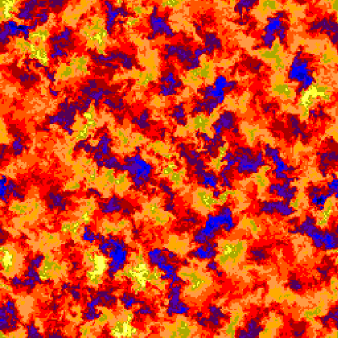
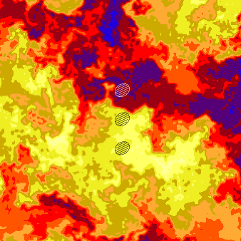
Figure 3: Left : Typical snapshots of the scalar field $\theta$. Note the presence of sharp fronts separating large regions in which the scalar assumes close values. Right : Close-up of a region containing a front. Across the upper and the middle spot there is a front, whereas the middle and lower one lie in a plateau. The distance between consecutive spots is larger than the diffusive scale $L_{\kappa}$, but smaller than the injection scale $L_{\phi}$. In this simulation $L_{\kappa}\approx 2$ , $L_{\phi}\approx 170$, the spot separation and diameter are $\approx 25$ and $\approx 15$, respectively. Lengths are expressed in grid points.

A striking and ubiquitous feature of passive scalar turbulence is the presence of fronts (also called “cliffs” or “sheets”), i.e. regions where the scalar has very strong variations separated by large regions (“ramps” or “plateaux”) where scalar fluctuations are weak (see Fig. 3) [8, 9, 10, 11, 12, 13, 14, 15, 16].

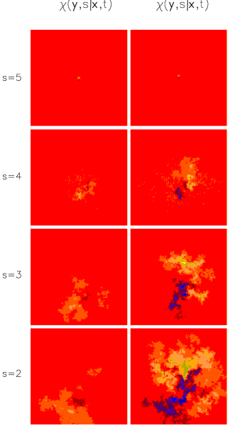
Figure 4: From top to bottom : backward evolution of $\chi({\bm{y}},s|{\bm{x}},t)$ for ${\bm{x}}$ and ${\bm{r}}$ starting in a plateau (first column) and across a front (second column), see the right panel of Fig. 3. Colors are coded according to the intensity of the field $\chi$, yellow is for positive values and blue for negative ones. At each time, the intensity is normalized according to the maximum of the fields in absolute value. The relatively smaller intensity on the first column is due to the fast mixing leading to strong cancellations between the positive and negative parts. Time is in eddy turnover times, the total number of time steps is $2^{14}$. To compare with figure 3, here the panel is $900\times 900$ grid points.

The genesis of fronts and plateaux is best understood in terms of particle trajectories : to trace back the build-up of large and small scalar difference we study the evolution of the propagator

$$\chi({\bm{y}},s|{\bm{x}},{\bm{x}}+{\bm{r}},t)=P({\bm{y}},s|{\bm{x}}+{\bm{r}},t)-P({\bm{y}},s|{\bm{x}},t)\;,$$ (10)

which is related to the scalar difference by the formula

$$\theta({\bm{x}}+{\bm{r}},t)-\theta({\bm{x}},t)=\int_{0}^{t}\!\!\d s\int\!\!\d{\bm{y}}\;\chi({\bm{y}},s|{\bm{x}},{\bm{x}}+{\bm{r}},t)\,\phi({\bm{y}},s)\;.$$ (11)

Notice that $\chi$ evolves backward according to Eq. (4), with the final condition $\chi({\bm{y}},s|{\bm{x}},{\bm{x}}+{\bm{r}},t)=\delta({\bm{y}}-{\bm{x}}-{\bm{r}})-\delta({\bm{y}}-{\bm{x}})$.

The numerical procedure was as follows. After the integration of Eqs. (5) and (8) over five eddy turnover times (the typical time-scale of large-scale motion) we choose ${\bm{x}}$ and ${\bm{r}}$ such that ${\bm{x}}$, ${\bm{x}}+{\bm{r}}$ are on a front or a plateau, respectively (see the right panel of Fig. 3). Then $\chi$ is integrated backward in time. In Fig. 4, we show four snapshots of the backward evolution of the field $\chi$. Already at a first glance the evolution of $\chi$ appears very different for the two final conditions : the blobs starting inside a plateau (first column) experience a strong mixing, while blobs lying initially across a front mix very poorly remaining compact and far aside. This is the basic mechanism for the formation of intense structures in passive scalar turbulence (for a related theoretical study see [17]).

References

- [1] H. Risken, The Fokker Planck Equation (Springer-Verlag, New York/Berlin, 1996).
- [2] C. W. Gardiner, Handbook of Stochastic Methods : For Physics, Chemistry and the Natural Sciences (Springer-Verlag, New York/Berlin, 1996).
- [3] B. I. Shraiman and E. D. Siggia, Scalar turbulence, Nature 405, 639 (2000).
- [4] G. Falkovich, K. Gawȩdzki, and M. Vergassola, Particles and fields in fluid turbulence, Rev. Mod. Phys. 73, 913 (2001).
- [5] D. Gottlieb and S.A. Orszag, Numerical Analysis of Spectral Methods : Theory and Applications, (SIAM, Philadephia, 1977).
- [6] C. Canuto, M. Y. Hussaini, A. Quarteroni and T. A. Zang, Spectral methods in fluid dynamics, (Springer-Verlag, New York/Berlin, 1988).
- [7] G. Boffetta, A. Celani, and M. Vergassola, Inverse energy cascade in two-dimensional turbulence : Deviations from Gaussian behavior, Phys. Rev. E 61, 29 (2000).
- [8] A. Celani, A. Lanotte, A. Mazzino, and M. Vergassola, Universality and Saturation of Intermittency in Passive Scalar Turbulence, Phys. Rev. Lett. 84, 2385 (2000).
- [9] A. Celani, A. Lanotte, A. Mazzino, and M. Vergassola, Fronts in passive scalar turbulence, Phys. Fluids 13, 1768 (2001).
- [10] F. Dalaudier, C. Sidi, M. Crochet, and J. Vernin, Direct evidences of “sheet” in the atmospheric temperature field, J. Atmos. Sci. 51, 237 (1994).
- [11] R. G. Luek, Turbulent mixing at the Pacific subtropical front, J. Phys. Oceanogr. 18, 1761 (1988).
- [12] K. R. Sreenivasan, On local isotropy of passive scalars in turbulent shear flows, Proc. Roy. Soc. London A434, 165, (1991).
- [13] L. Mydlarski and Z. Warhaft, Passive scalar statistics in high-Péclet-number grid turbulence, J. Fluid Mech. 358, 135, (1998).
- [14] F. Moisy, H. Willaime, J. S. Andersen, and P. Tabeling, Passive Scalar Intermittency in Low Temperature Helium Flows, Phys. Rev. Lett. 86, 4827 (2001).
- [15] A. Pumir, A numerical study of the mixing of a passive scalar in three dimensions in the presence of a mean gradient, Phys. Fluids 6, 2118 (1994).
- [16] S. Chen and R. H. Kraichnan, Simulations of a randomly advected passive scalar field, Phys. Fluids 68, 2867 (1998).
- [17] E. Balkovsky and V. Lebedev, Instanton for the Kraichnan passive scalar problem, Phys. Rev. E 58, 5776 (1998).