Coulomb scattering in plasma revised

Abstract

A closed expression for the momentum evolution of a test particle in weakly-coupled plasma is derived, starting from quantum many particle theory. The particle scatters from charge fluctuations in the plasma rather than in a sequence of independent binary collisions. Contrary to general belief, Bohr’s (rather than Bethe’s) Coulomb logarithm is the relevant one in most plasma applications. A power-law tail in the distribution function is confirmed by molecular dynamics simulation.

Though Coulomb scattering is a most basic process in plasma and has been studied for a century Bohr , doubts concerning the treatment as a sequence of independent binary collisions remained Kog ; Siv , and recent analysis Gor has revealed that this standard assumption is not justified in general and requires revision. Here we derive the time-dependent many-particle wavefunction of a test particle simultaneously interacting with $N$ particles residing in the Debye sphere. The plasma parameter $N=n\lambda^{3}>1$ involves the plasma density $n$ and the screening length $\lambda=max(v_{T}/\omega_{p},v_{0}/\omega_{p})$, where $v_{T}$ is the thermal velocity of electrons, $v_{0}$ the velocity of the test particle, and $\omega_{p}=\sqrt{4\pi ne^{2}/m_{e}}$ the plasma frequency. We emphasize that the collective interaction described here is different and in addition to Debye screening; it is not included in the usual dielectric approach Larkin . The new results can be viewed as interaction of the test particle with the charge fluctuations inside the Debye sphere; in this picture, the test particle of charge $Z_{0}e$ is scattered by an effective, spatially extended charge $e\sqrt{N}$ rather than by a sequence of binary collisions.

This has deep consequences for the Coulomb logarithm, because it drastically shifts the borderline between classical and quantum Coulomb scattering, extending the domain in which the classical approximation applies. This is shown in Fig. 1. In the binary collision approach (Fig. 1a), the borderline is given by the parameter $\alpha=Z_{0}e^{2}/\hbar v_{0}$ such that $\alpha<1$ defines the quantum-mechanical region where the Born approximation leads to Bethe’s logarithm $L_{q}=\ln(\lambda m_{e}v_{0}/\hbar)$ Bethe , while for $\alpha>1$ classical mechanics apply leading to Bohr’s logarithm $L_{cl}=\ln(\lambda m_{e}v_{0}^{2}/Z_{0}e^{2})$. In the present theory instead, the borderline is given by $\alpha N^{1/2}\approx 1$, and this leads to a very different picture in Fig.1b. Now $L_{cl}$ applies to almost the entire high-temperature region, including e.g. the important domain of magnetic fusion plasmas, while $L_{q}$ plays only a marginal role.

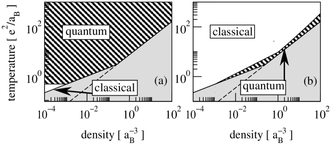
Figure 1: Regions in a density-temperature plane (atomic units) in which Bohr’s classical Coulomb logarithm (white area) and Bethe’s quantum expression (hatched area) apply; (a) binary collision theory with borderline defined by $\alpha=Z_{0}e^{2}/\hbar v_{0}=1$, and (b) present theory with approximate separation along $\alpha^{2}N(1+\ln N)=1$. Also shown as grey area are the region of strongly non-ideal plasma (borderline: $T\sim n^{1/3}$) and the region of degenerate plasma (borderline: $T\sim n^{2/3}$).

Let us first discuss this result in qualitative terms. A particular feature of the Coulomb ($1/r$) interaction is of crucial importance in this case, namely that scattering does not depend on $\alpha$ and $\hbar$, as we know from the Rutherford cross section. The difference between $\alpha<1$ and $\alpha>1$ regions arises only when the potential deviates from $1/r$, as it is the case in a plasma due to Debye screening occurring at long distances $\lambda$. This means the distinction between classical and quantum treatment reveals itself for small-angle scattering, while close collisions with large-angle scatter are not affected. This point has been emphasized strongly by Bohr (see p.448 in Bohr ) and also in Sivukhin’s review Siv (p. 109–113). In accordance with Bohr “any attempt to attribute the difference between [the classical $\alpha\gg 1$ and quantum $\alpha\ll 1$ cases] to the obvious failure of [the classical] pictures in accounting for collisions with an impact parameter smaller than [the de Broglie wave–length] will be entirely irrelevant. In fact, this argument would imply a difference between two distribution for the large angle scattering, while the actual differences occur only in the limits of small angles.”

Now let us compare the classical scattering angle $\delta_{cl}=(Z_{0}e\,e_{*}/m_{0}v_{0}^{2})/\lambda$ at distance $\lambda$ with that of quantum diffraction $\delta_{q}=(\hbar/m_{0}v_{0})/\lambda$ Lan . The open question here concerns the effective net charge $e_{*}$ which the test particle experiences when passing the Debye sphere. The value of $e_{*}$ is not evident, because we are dealing with Coulomb collisions at distances much larger than $1/n^{1/3}$. The binary collision approximation circumvents this predicament by alleging that the total scattering can be treated as the sum of independent binary interactions happening at different times Siv . One is then led to take $e_{*}=e$ for granted instead of actually calculating $e_{*}$. The central result of this paper will be that the effective charge is essentially given by $e_{*}\approx eN^{1/2}$. The matching condition then is $\delta_{cl}/\delta_{q}\approx\alpha N^{1/2}\approx 1$ replacing the condition $\alpha\approx 1$ obtained in binary collision approximation Siv . The theory underlying Fig. 1b will now be derived. As a central result, we also present molecular dynamics simulations confirming the analytic theory.

The present analysis starts from a full quantum-mechanical description of the plasma in terms of the many-particle wave-function $\psi=\exp(iS/\hbar)$. The action function $S$ satisfies the equation

$$-\frac{\partial S}{\partial t}=\sum_{j}\left(\frac{(\nabla_{j}S)^{2}}{2m_{j}}+\sum_{k>j}U_{j,k}-i\hbar\frac{\Delta_{j}S}{2m_{j}}\right),$$ (1)

where the indices $j$ and $k$ denote plasma particles for $j,k=1,2,3\dots$ and the test particle for $j,k=0$, $m_{j}$ are the masses, and $U_{j,k}$ represent the Coulomb interactions. Eq. (1) is equivalent to the exact Schrödinger equation and has the form of a Hamilton-Jacoby equation with additional terms that are proportional to $\hbar$ and describe quantum effects. We examine the solution of Eq. (1) for the particular initial conditions $S(t=0)=\sum_{j\geq 0}{\bf p}_{j}\cdot{\bf r}_{j}$, (the Green function for the coordinate–momentum representation). where ${\bf p}_{j}$ are given momenta of the plasma particles at $t=0$, and introduce

$$\sigma=S-\sum_{j\geq 0}\left({\bf p}_{j}\cdot{\bf r}_{j}-{\bf p}_{j}^{2}t/2m_{j}\right)$$

such that $\sigma(t=0)=0$. Now the clue for solving Eq.(1) is the high-energy approximation Lan which applies to an almost ideal plasma and requires $|{\bf p}_{j}|\gg|\nabla_{j}\sigma|$. Under this approximation we find

$$-\frac{\partial\sigma}{\partial t}=\sum_{j}\left({\bf v}_{j}\cdot\nabla_{j}\sigma+\sum_{k>j}U_{j,k}-i\hbar\frac{\Delta_{j}\sigma}{2m_{j}}\right),$$ (2)

where ${\bf v}_{j}={\bf p}_{j}/m_{j}$. The solution of Eq. (2) for $\sigma(t=0)=0$ is

$$\sigma=-\sum_{j\geq 0}\sum_{k>j}\int_{0}^{t}U_{k,j}\left({\bf D}_{k,j}\right)\,d\tau,$$ (3)

where $\delta{\bf r}_{k,j}={\bf r}_{k}-{\bf r}_{j}$, $\delta{\bf v}_{k,j}={\bf v}_{k}-{\bf v}_{j}$ and ${\bf D}_{k,j}=\delta{\bf r}_{k,j}-\delta{\bf v}_{k,j}(t-\tau)$. It can be verified by direct insertion. The terms $\Delta_{j}\sigma$ proportional to $\hbar$ vanish for the special case of Coulomb $U\propto 1/|{\bf D}|$ interactions for distances $|{\bf D}|>0$.

The problem of solution (3) is that it contains the singularities of $U_{k,j}({\bf D}_{k,j})$ for close encounters with $|{\bf D}_{k,j}|\rightarrow 0$. This deficiency is due to the high energy approximation. Inserting Eq. (3) into $|{\bf p}_{j}|\gg|\nabla_{j}\sigma|$, we find that this condition is fulfilled only for regions

$$|{\bf D}_{k,j}|>|e_{j}e_{k}|/(\mu_{k,j}|\delta{\bf v}_{k,j}|^{2})$$ (4)

with $0<\tau<t$ and $\mu_{k,j}=m_{j}m_{k}/(m_{j}+m_{k})$. Had we solved the nonlinear equation (1) exactly, we had obtained a non–singular result with the maximum momentum transfer of $2\delta v_{j,k}\mu_{j,k}$, as we know from Rutherford scattering. The way to deal with this problem is to cut out in the wavefunction those spatial regions which do not satisfy Eq. (4). The cut-off (4) warrants that the maximum momentum transfer $2\delta v_{j,k}\mu_{j,k}$ is preserved; this can be verified by operating with $-i\hbar\nabla_{j}$ on $\exp(iS/\hbar)$. It should be understood that this short-range cut-off is a technical correction (compare with Bohr , p. 448–449:”…the central region of the field…, which, on classical mechanics, is responsible for all large angle scattering will, for $\alpha\ll 1$,…gives rise to only a fraction of the order $\alpha^{4}$ of the Rutherford scattering”). It has nothing in common with differences between classical and quantum scattering. These reveal themselves only at long ranges Bohr ; Siv . Another detail concerning the general wavefunction concerns the initial conditions. In case the initial state of the plasma is defined by the wavefunction $\phi(t=0,{\bf p}_{1},{\bf p}_{2},\dots)$ rather than by a fixed set of momenta, the corresponding general wavefunction is given by

$$\psi(t,{\bf r}_{0},{\bf r}_{1},\dots)=\int\exp(iS/\hbar)\phi(t=0,{\bf p}_{1},{\bf p}_{2},\dots)\prod_{k\geq 1}\,d{\bf p}_{k}.$$

As it turns out, the explicit form of $\phi$ is of no relevance in the applications discussed below.

We now have at our disposal in analytical form the time-dependent many-particle wavefunction describing a dilute high-temperature plasma. This is a remarkable result. An outstanding feature is that it describes simultaneous multiple Coulomb interactions between the particles and, in this respect, goes beyond the binary collision approximation. Another essential property is that it holds for both the quasi-classical regime ($\sigma\gg\hbar$) as well as the deeply quantum-mechanical regime ($\sigma\ll\hbar$) and therefore provides a unique tool to investigate the transitional region. We now proceed to use this wavefunction to calculate plasma properties. This is straightforward, though tedious, and therefore we can give here only the main results, leaving technical derivations to a separate publication.

We first consider the distribution function ${M}(t,{\bf Q})$ of transverse momentum ${\bf Q}$ of a test particle moving at time $t=0$ with momentum ${\bf p}$ collinear to the $x$-axis. For brevity we consider a fast ion $m_{0}\gg m_{e}$ , $v_{0}\gg v_{T}$ for times that are longer than $t_{0}=\lambda/v_{0}$, though shorter than the collision time $t_{c}\sim m_{0}Nt_{0}/m_{e}L_{cl,q}$. ${M}(t,{\bf Q})$ is obtained as the matrix element

$$M(t,{\bf Q})=\int\exp\left(i{\bf Q}\cdot{\bf R}/\hbar\right)F(t,{\bf R})\,d^{2}{\bf R}/(2\pi\hbar)^{2}$$ (5)

where

$$F(t,{\bf R})=\frac{1}{V}\int\psi(t,{\bf r}_{0},{\bf r}_{1},\dots)\psi^{*}(t,{\bf r}_{0}+{\bf R},{\bf r}_{1},\dots)\prod_{k\geq 0}\,d^{3}{\bf r}_{k}$$

and $V$ is the plasma volume.

Expression (5) can be significantly simplified for the case under consideration. The test particle affects only plasma particles in the interaction sphere $|\delta{\bf r}_{0,j}|<\lambda$, for which two–particle correlations among plasma particles are small owing to $T\gg e^{2}n^{1/3}$. Aiming deliberately for calculations with logarithmic accuracy, we can omit the integration over $|\delta{\bf r}_{0,j}|>\lambda$ and use the method developed in Gor . We find $F(t,{\bf R})=F_{e}(t,{\bf R})F_{i}(t,{\bf R})$ where $F_{e}(t,{\bf R})=\exp(-f_{e}(t,{\bf R}))$,

$$f_{e}=2N\int\sin^{2}\left[\frac{\alpha}{4}\left(g(t,{\bf r}_{0}+{\bf R})-g(t,{\bf r}_{0}\right)\right]\frac{d^{3}{\bf r}_{0}}{\lambda^{3}},$$ (6)

$$g=\int_{-v_{0}t}^{v_{0}t}V_{0}(x_{0}+\zeta/2-v_{0}t,y_{0}+Y,z_{0}+Z)\,d\zeta,\$$ (7)

$N=n\lambda^{3}$, $\alpha=Z_{0}e^{2}/\hbar v_{0}$, ${\bf r}_{0}=(x_{0},y_{0},z_{0})$, $V_{0}({\bf r}_{0})=1/|{\bf r}_{0}|$ for $|{\bf r}_{0}|<\lambda$ and $V_{0}=0$ for $|{\bf r}_{0}|>\lambda$. In the ${\bf r}_{0}$–integration, the domain $\min((y_{0}+Y)^{2}+(z_{0}+Z)^{2},y_{0}^{2}+z_{0}^{2})<r^{2}_{cl}=(Z_{0}e^{2}/m_{e}v_{0}^{2})^{2}$ is excluded for reasons discussed above. The ion function $F_{i}$ has the same structure as $F_{e}$ and is simply obtained by substituting ion parameters. ${M}$ is the convolution of ${M}_{e}$ and ${M}_{i}$, where

$${M}_{e,i}(t,{\bf Q})=\int\exp(i{\bf Q}\cdot{\bf R}/\hbar)F_{e,i}(t,{\bf R})\,d^{2}{\bf R}/(2\pi\hbar)^{2}$$

are the transverse momentum distributions due to the electron–projectile and ion–projectile interaction. In the following, most of the discussion is restricted to $M_{e}$.

Let us discuss the structure of Eqs. (6),(7), which are presented here for the first time. The detailed analysis is quite intricate, and here we give only the main results without derivation. We observe that only small enough $f_{e}$ can contribute to $M$ and that therefore, owing to the large multiplier $N$ in Eq. (6), the sin²-term needs to be small and can be expanded. Then $M$ depends essentially on the parameter combination $\alpha^{2}N$ only; more rigorous analysis gives $\gamma=\alpha^{2}N\ln N$. The quantum regime is restricted to $\gamma<1$, while the classical regime is found for $\gamma>1$ and will be discussed first. Evaluating Eq. (6) in the limit of very small $R$, one finds $f_{e}({\bf R})=\nu t\ln(\lambda m_{e}v_{0}^{2}/Z_{0}e^{2})({\bf R}/\hbar)^{2}$ with $\nu={2\pi nZ_{0}^{2}e^{4}}/v_{0}$. This is the relevant region in the Fourier integral of ${M}_{e}$ for large enough time $t$ ($t_{1}\ll t<t_{c}$, see below). The function $F_{e}({\bf R})$ is then a Gaussian, and ${M}_{e}$ can be easily calculated. Setting $F_{i}=1$, we obtain $\left<Q^{2}\right>_{e}=\int{\bf Q}^{2}M_{e}(t,{\bf Q})\,d^{2}{\bf Q}=4\nu tL_{cl}$ and recover the classical Coulomb logarithm $L_{cl}=\ln(\lambda m_{e}v_{0}^{2}/Z_{0}e^{2})$. The important new result here is that it applies to the whole region $\gamma>1$ and not just to $\alpha>1$.

It should be noticed, however, that the function $f_{e}({\bf R})=\nu t\ln(\lambda/{\tilde{R}})({\bf R}/\hbar)^{2}$ is more complicated in general and contains a factor $\ln{\tilde{R}}$ for larger radii, where ${\tilde{R}}=\max(\alpha|{\bf R}|,\alpha\hbar/m_{e}v_{0})$ for $\alpha>1$ and ${\tilde{R}}=\max(|{\bf R}|,\alpha\hbar/m_{e}v_{0})$ for $\alpha<1$. For short times, just somewhat larger than $\lambda/v_{0}$, this logarithmic factor modifies the Gaussian character of $M_{e}(t,{\bf Q})$, giving it a power–law tail at high $Q=|{\bf Q}|$. We then obtain

$$M(t,{\bf Q})=\exp(-Q^{2}/2p_{0}^{2})/(2\pi p_{0}^{2})$$ (8)

for $Q^{2}<2p_{0}^{2}\ln\Lambda$ and

$$M(t,{\bf Q})=2p_{0}^{2}/(\pi\Lambda Q^{4})$$ (9)

for $2p_{0}^{2}\ln\Lambda<Q^{2}<(2m_{e}v_{0})^{2}$, where $\Lambda$ is a solution of $\Lambda=\ln(2\pi\alpha_{1}n\Lambda\lambda^{2}v_{0}t)\gg 1$, $\alpha_{1}=\min(1,\alpha)$ and $p_{0}^{2}=\nu\Lambda t$. Physically, the Gaussian distribution at small $Q$ corresponds to small angle scattering and the power–law tail to close collisions with large momentum transfer. The tail is obtained only as long as $t<t_{1}=2m_{e}^{2}v_{0}^{2}/\nu\Lambda\ln\Lambda$, such that $2p_{0}^{2}\ln\Lambda<(2m_{e}v_{0})^{2}$. For longer times, small angle scattering dominates both small and large $Q$ regions and the tail disappears.

We have checked the occurrence of this power-law tail by molecular dynamics (MD) simulations. We consider a test particle with $v_{0}\gg v_{th}$ scattered completely classically in a finite plasma volume, having dimensions $l$ of the order of the screening length. The simulation has been performed for a model case with $N=80$ and $\alpha=1.9$, just feasible on a modern PC. Results are plotted in Fig. 2 for time $t=2l/v_{0}<t_{1}$ . The histogram presenting the MD results is in best agreement with the present theory (solid curve), clearly showing the power-law tail at high momenta. For comparison, also the purely Gaussian distribution obtained from the Landau collision integral is given as dashed line. Details of these simulations are outlined in the caption.

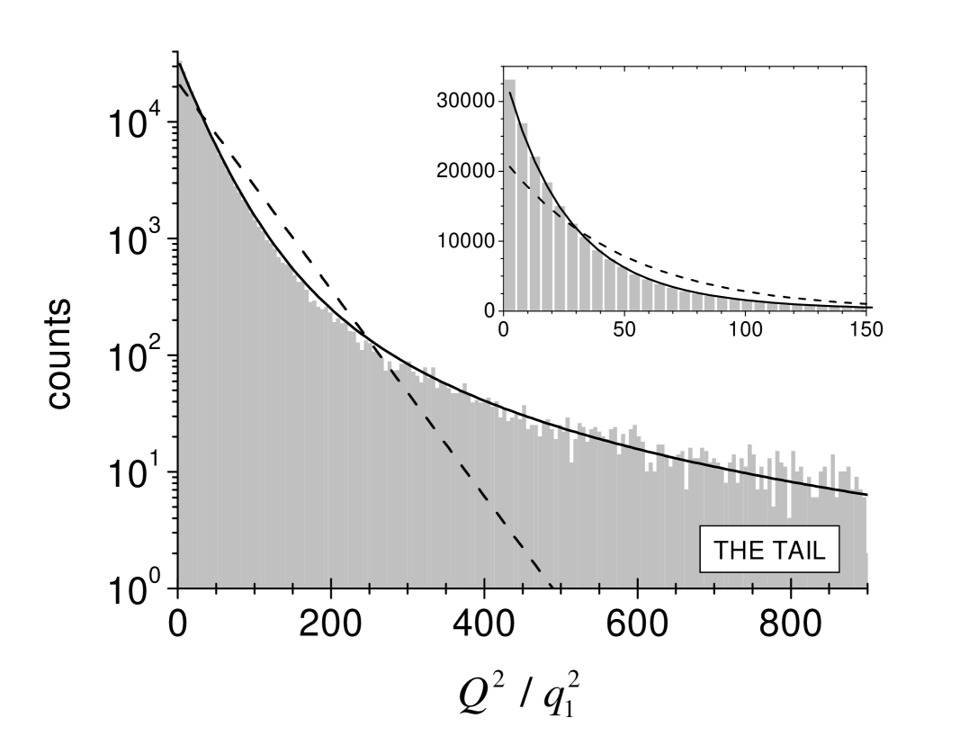
Figure 2: Comparison between MD simulation (histogram), present theory (solid line), and predictions of the traditional diffusion approximation (dashed line); $\pi M(t,Q)$ is plotted versus $Q^{2}/q_{1}^{2}$ for time $t=2l/v_{0}$, $l=7.239\times 10^{-6}$cm, velocity of test particle $v_{0}=2.297\times 10^{8}$cm/s, and $q_{1}^{2}=2\pi nZ_{0}^{2}e^{4}t/v_{0}$. The insert shows the same plot, but with linear scale and zoomed to low $Q$. The simulation assumes an equal number of randomly distributed, fixed Coulomb centers of opposite charge $\pm e$ and densities $n_{+}=n_{-}=n=1.054\times 10^{17}$ cm^-3; the cold plasma limit is chosen with thermal velocity $v_{th}\ll v_{0}$. The plasma volume is taken as $V=6l\times 2l\times 2l$ with the test particle ($Z_{0}=2$, $m_{0}=m_{e}$) moving along the central axis in $x$-direction and starting at a distance $2l$ from the surface. The trajectory of the test particle, interacting with all Coulomb centers, is obtained by solving the classical equation of motion by a second-order scheme with an adaptive time step. The histogram corresponds to $2.06\times 10^{5}$ independent trials. The solid line has been obtained numerically from Eqs. (6)–(7) with $F_{i}=F_{e}=\exp(-f_{e})$. The screening length is set to $\lambda=l$ such that the finite plasma volume seen by the test particle in this model simulation just mimics the physically screened volume occuring in reality. The straight dashed line is the Landau collision integral prediction $M(t,Q)=\exp(-Q^{2}/Q_{0}^{2})/(\pi Q_{0}^{2})$ with $Q_{0}^{2}=8\pi e^{4}Z_{0}^{2}(n_{+}+n_{-})L_{0}t/v_{0}$; $L_{0}=6.5$ is the classical Coulomb logarithm evaluated for the parameters of the simulation.

Here we should make it clear that the power law tail originating from close collisions is obtained in nearly identical form within the binary collision approach, as it was shown by Landau Landau and Vavilov Vavilov . The present theory differs for small-angle scattering and therefore in the Gaussian part of $M(t,Q)$. To show the difference quantitatively, we have also solved the kinetic equation used in Landau ; Vavilov . The result can be written in a form equivalent to Eq. (5) with the function $f_{e}$ now given approximately by $f_{e}^{(b)}=\nu t\ln(\alpha_{1}\lambda/{\tilde{R}})({\bf R}/\hbar)^{2}$, where ${\tilde{R}}=\max(\alpha|{\bf R}|,\alpha\hbar/m_{e}v_{0})$ and $\alpha_{1}=\min(1,\alpha)$. The effect of the present theory is that the Gaussian part grows more rapidly. This is consistent with enhanced small-angle scattering due to simultaneous interaction with many plasma particles.

We have seen in Fig. 1 that the quantum limit ($\gamma<1$) is relevant only in a marginal parameter region. Nevertheless, it is contained in $M_{e}$. For $\gamma<1$, one can use first-order expansions of $F_{e}=1-f_{e}$ and of the sin²-term in $f_{e}$ to find, after some algebra, $M_{e}(t,{\bf Q})=C(t)\delta({\bf Q})+\sigma(Q)nvt/(m_{e}v)^{2}$, where $C(t)=1-nvt/(m_{e}v_{0})^{2}\int\sigma(Q)\,d^{2}{\bf Q}$ and $\sigma(Q)\approx r_{cl}^{2}(2m_{e}v_{0})^{4}/(Q^{2}+(\hbar/\lambda)^{2})^{2}$ is the cross–section of the screened Coulomb potential. This leads to $\left<Q^{2}\right>_{e}=4\nu tL_{q}$ and the quantum (Bethe) logarithm $L_{q}=\ln(\lambda m_{e}v_{0}/\hbar)$. This first-order Born result is obtained here for $\alpha N^{1/2}<<1$, but not for $\alpha<1$ in general. This may be understood qualitatively looking at second-order processes. Consider the perturbation of the interaction of the test particle with a plasma particle $j$ by another plasma particle $k$. This effect is small of order $\alpha^{2}$, but since for a plasma with long–range Coulomb forces $N$ particles contribute to this second-order process, it can be neglected only if $\alpha^{2}N<1$.

Let us finally calculate the energy ${\mathcal{E}}(t)=\left<\psi\left|{\hat{H}}_{p}\right|\psi\right>$ the plasma gains due to the energy loss of the test particle. Here

$${\hat{H}}_{p}=\sum_{j\geq 1}\left(-\hbar^{2}\Delta_{j}/(2m_{j})+\sum_{k>j}U_{j,k}\right)$$

is the Hamiltonian of the plasma without the test particle Larkin and $\psi(t,{\bf r_{0}},{\bf r}_{1},\dots)$ the full wavefunction. Making use of the same approximations as in the derivation of Eq. (5), straightforward algebra leads to $d{\mathcal{E}}/dt=\left<Q^{2}\right>_{e}/2m_{e}+\left<Q^{2}\right>_{i}/2m_{i}$, where the first term is the contribution from plasma electrons with mass $m_{e}$ and the second from ions with mass $m_{i}$. The corresponding electron part of the stopping power is then found in the standard form

$$\frac{dE}{dx}=-\frac{1}{v_{0}}\frac{d{\mathcal{E}}}{dt}=-\frac{4\pi ne^{4}Z_{0}^{2}}{m_{e}v_{0}^{2}}L,$$

but now with $L=L_{cl}$ for $\gamma>1$ and $L=L_{q}$ for $\gamma<1$.

In conclusion, it has been shown that the theory of Coulomb scattering in dilute plasma needs revision. Bohr’s classical Coulomb logarithm $L_{cl}$ is found to apply for $\alpha\sqrt{N}>1$ rather than $\alpha>1$, and this covers most of the density-temperature plane, relevant to practical applications. This result calls for experimental verification. We propose to measure energy loss of fully stripped ions in carefully characterized, fully ionized plasma layers. The parametrically different dependence of $L_{cl}$ and $L_{q}$ on ion charge $Z_{0}$ and velocity $v_{0}$ should allow for a clear distinction.

References

(1)
N. Bohr,
The penetration of atomic particles through matter
Math.-Fys. Medd XVIII (1948) (reprinted in Niels Bohr
Collected Works,
J. Thorsen,
Vol 8,
Amsterdam,North-Holland,
1987,
page 425.