Nematic Ordering of Rigid Rods in a Gravitational Field

Abstract

The isotropic-to-nematic transition in an athermal solution of long rigid rods subject to a gravitational (or centrifugal) field is theoretically considered in the Onsager approximation. The new feature emerging in the presence of gravity is a concentration gradient which coupled with the nematic ordering. For rodlike molecules this effect becomes noticeable at centrifugal acceleration $g\sim 10^{3}\div 10^{4}$ m/s², while for biological rodlike objects, such as tobacco mosaic virus, TMV, the effect is important even for normal gravitational acceleration conditions. Rods are concentrated near the bottom of the vessel which sometimes leads to gravity induced nematic ordering. The concentration range corresponding to phase separation increases with increasing $g$. In the region of phase separation the local rod concentration, as well as the order parameter, follow a step function with height.

I Introduction

Nematic ordering in a solution of long rigid rods has been studied theoretically in many papers, starting from the classical papers by Onsager 1 and Flory 2 . However, there is one aspect of this problem, which has never been considered, namely that this transition always occurs in a gravitational field. This field induces a concentration inhomogeneity within the volume where nematic ordering takes place. Such inhomogeneity should, in principle, change some of the characteristics of the liquid-crystalline transition.

The dimensionless parameter associated with gravitational field is $\beta\equiv mgh/kT$ where $m=m_{0}-\widetilde{\rho}v$ is the mass of a rod corrected for buoyancy ($\widetilde{\rho}$ and $v$ are the density of pure solvent and the volume of the rod, respectively), $h$ is the height, $g$ is the gravitational acceleration, $T$ is the temperature and $k$ is the Boltzmann constant. For $h=1$ cm and room temperature conditions, this gives the following criterion: the inhomogeneity due to the normal gravitational acceleration ($9.8$ m/s²) becomes important for molecular masses of rod more than $10^{7}$ g/mol. Thus, for rigid rods made of common synthetic macromolecules ($m_{0}\sim 10^{5}$ g/mol) this effect can be neglected.

However, in at least two situations the effect of gravity on the problem of the liquid crystalline transition is important and experimentally relevant. First, for nematic ordering in solutions of high molecular weight rodlike biological objects (such as TMV or virus fd) 3 ; 4 ; 5 ; 6 ; 7 $m$ can be very large ($m_{0}=4\times 10^{7}$ g/mol for TMV,4 ), and values of $\beta>1$ can easily be reached. Second, instead of normal gravitational acceleration, one can consider the acceleration in an ultracentrifuge which can be $10^{4}\div 10^{5}$ times larger than ordinary gravity. For at least these cases, the investigation of the influence of gravitational field on the nematic ordering in the solution of rigid rods seems to be an important problem. This problem is solved theoretically below in the Onsager approximation.

II Theoretical model

The Onsager approach is based on a virial expansion of the free energy of the solution of rigid rods taking into account steric repulsion only.

Let us choose the Cartesian coordinate system in such a way that the external field acts in the z direction and put the origin of coordinates at the bottom of the reservoir (z=0). Further, let us divide the volume of the vessel V into large number of identical layers aligned perpendicularly to the field in order that all particles in a given layer has the same gravitational potential. Here we use the following notation: $dN_{z}\left(\Omega\right)=N_{z}f_{z}\left(\Omega\right)d\Omega$ is the number of rods in the layer z with axis directions within the small spatial angle $d\Omega$, $N_{z}$ is the total number of rods in the layer z, and $\zeta=z/h$ denotes the dimensionless height. Let $f_{z}\left(\Omega\right)$ be one-particle orientational distribution function of rods in the layer z. The normalization for the function $f_{z}\left(\Omega\right)$ is written in the familiar form $\int f_{z}\left(\Omega\right)d\Omega=1$.

With such division of the volume of the vessel into very large number of layers, the local rod concentration $C^{\prime}(\zeta)$ has the same value within the layer. Thus, for a given layer one can apply the traditional Onsager theory 1 , 8 ; 9 justified for homogeneous system. This theory is valid for dilute enough solutions of very long rods.

In this case, the local free energy of the layer labeled $\zeta$ is written as

$$\frac{\varpi(\zeta)}{kT}=\ln C^{{}^{\prime}}(\zeta)+\int f\left(\Omega,\zeta\right)\ln\left(4\pi f\left(\Omega,\zeta\right)\right)d\Omega+C^{{}^{\prime}}(\zeta)\int f\left(\Omega_{1},\zeta\right)f\left(\Omega_{2},\zeta\right)a_{2}\left(\gamma\right)d\Omega_{1}d\Omega_{2}+\int\beta\zeta f\left(\Omega,\zeta\right)d\Omega$$ (1)

where the first term represents the entropy of a translational motion, the second term is the orientation entropy, the third term describes steric interaction of rods in the second virial approximation, and the last term is the average potential energy of a rod in an external gravitational field $U_{ext}\left(\zeta\right)/kT=\frac{mgh}{kT}\zeta\equiv\beta\zeta$.

To calculate the third term one assumes that the $\gamma$-dependent second virial coefficient $a_{2}$ is the half of excluded volume of two rods 1 , thus, $a_{2}\left(\gamma\right)=L^{2}D\left|\sin\gamma\right|$, where $L$ and $D$ are the length and diameter for long rigid rods and $\gamma$ is the angle between directions of long axes.

The free energy of the whole system is a sum of free energies of all layers. If the number of layers is large enough, the sum can be replaced by integral

$$\frac{F}{VkT}=\int_{0}^{1}d\zeta C^{{}^{\prime}}(\zeta)\frac{\varpi(\zeta)}{kT}=\int_{0}^{1}d\zeta C^{{}^{\prime}}(\zeta)\left(\ln C^{{}^{\prime}}(\zeta)+\sigma(\zeta)+C^{{}^{\prime}}(\zeta)\rho^{{}^{\prime}}(\zeta)+\beta\zeta\right)$$ (2)

where

$$\sigma(\zeta)\equiv\int f\left(\Omega,\zeta\right)\ln\left(4\pi f\left(\Omega,\zeta\right)\right)d\Omega$$ (3)

is the orientational entropy of the layer $\zeta$ and

$$\rho^{\prime}(\zeta)=\int f\left(\Omega_{1},\zeta\right)f\left(\Omega_{2},\zeta\right)a_{2}\left(\gamma\right)d\Omega_{1}d\Omega_{2}$$ (4)

is the second virial coefficient of interaction of two rods.

To obtain the equilibrium distribution function we should take into account the possibility of the formation of a phase boundary between the nematic phase at the bottom of the vessel and isotropic phase on top. We denote the height of the boundary position in the vessel as $\zeta=x$, so the volumes occupied by the nematic and isotropic phases are $V_{a}=xV$ and $V_{i}=\left(1-x\right)V$, respectively. With this, the free energy of the whole system eq. (2) becomes

$$\frac{F}{VkT}=\int_{0}^{x}d\zeta C_{a}^{{}^{\prime}}(\zeta)\frac{\varpi_{a}(\zeta)}{kT}+\int_{x}^{1}d\zeta C_{i}^{{}^{\prime}}(\zeta)\frac{\varpi_{i}(\zeta)}{kT},$$ (5)

where

$$\frac{\varpi_{a}(\zeta)}{kT}=\ln C_{a}^{{}^{\prime}}(\zeta)+\sigma_{a}(\zeta)+C_{a}^{{}^{\prime}}(\zeta)\rho_{a}^{{}^{\prime}}(\zeta)+\beta\zeta$$ (6)

is the local free energy of the nematic phase, and

$$\frac{\varpi_{i}(\zeta)}{kT}=\ln C_{i}^{{}^{\prime}}(\zeta)+\sigma_{i}(\zeta)+C_{i}^{{}^{\prime}}(\zeta)\rho_{i}^{{}^{\prime}}(\zeta)+\beta\zeta$$ (7)

is the local free energy of the isotropic phase.

To calculate the equilibrium distribution function $f\left(\Omega,\zeta\right)$ one should minimize the functional (5) with respect to this function. The direct minimization of functional (5) leads to a nonlinear integral equation, which can be solved only numerically 10 ; 11 . In the case where the volume of the vessel consists of two phases separated by a phase boundary, one should realize that $f\left(\Omega,\zeta\right)$ follows a step function with the variation of $\zeta$ with the function $f_{a}(\Omega,\zeta)$ in the anisotropic part significantly different from that in the isotropic phase $f_{i}(\zeta)=1/4\pi$. To evaluate the distribution function $f_{a}\left(\Omega,\zeta\right)$ in the nematic phase we apply an approximate variational method with a trial function depending on variational parameter $\alpha$.

Substituting this function in eqs. (5), (6), (7) and minimizing with respect to $\alpha(\zeta)$, we have the following equation for definition of variational function $\alpha(\zeta)$

$$\frac{d\sigma_{a}(\alpha)}{d\alpha}+C_{a}^{{}^{\prime}}(\zeta)\frac{d\rho_{a}^{{}^{\prime}}(\alpha)}{d\alpha}=0$$ (8)

However, the trial function proposed by Onsager 1 $f(\Omega,\alpha)=\left(\alpha/(4\pi\sinh\Theta)\right)\cosh\left(\alpha\cos\Theta\right)$, where $\Theta$ is the angular deviation of a rod from the director, still leads to rather complicated integral equation. Therefore, following 9 for the sake of simplicity we used a trial function of simpler form

$$f_{a}\left(\Omega,\alpha(\zeta)\right)=\frac{\alpha(\zeta)}{4\pi}\left\{\begin{array}[]{c}e^{-\frac{\alpha(\zeta)\Theta^{2}}{2}}\text{ },0<\Theta<\frac{\pi}{2}\\ e^{-\frac{\alpha(\zeta)(\pi-\Theta)^{2}}{2}},\frac{\pi}{2}<\Theta<\pi\end{array}\right.$$ (9)

with an approximate normalization (precise up to terms of order $O\left(e^{-\alpha}\right)$).

This trial function is suitable for approximate evaluation of $\sigma_{a}(\alpha(\zeta))$ in case of highly ordered state 9

$$\sigma_{a}\left(\alpha(\zeta)\right)\equiv\int f_{a}\left(\Omega,\alpha(\zeta)\right)\ln\left(4\pi f_{a}\left(\Omega,\alpha(\zeta)\right)\right)d\Omega\approx\ln\alpha(\zeta)-1,$$ (10)

and the dimensionless second virial coefficient in the anisotropic phase 9

$$\rho_{a}(\zeta)=\frac{\rho_{a}^{{}^{\prime}}(\zeta)}{b}=\frac{4}{\pi}\int f_{a}\left(\Omega_{1},\alpha(\zeta)\right)f_{a}\left(\Omega_{2},\alpha(\zeta)\right)\left|\sin\gamma\right|d\Omega_{1}d\Omega_{2}\approx\frac{4}{\sqrt{\pi\alpha(\zeta)}}$$ (11)

with notation $b\equiv\left\langle\left\langle\rho^{{}^{\prime}}(\zeta)\right\rangle_{i}\right\rangle_{i}=L^{2}D\left\langle\left\langle\left|\sin\gamma\right|\right\rangle_{i}\right\rangle_{i}=\frac{\pi}{4}L^{2}D$; the value of $b$ being equal to half of average excluded volume of two arbitrary oriented rods.

The corresponding expressions in the isotropic phase are

$$\sigma_{i}=0\text{ and }\rho_{i}=1\text{.}$$ (12)

In the above formulas the index $i$ and $a$ refers to the isotropic phase and the nematic phase respectively, and the angular brackets designate the average with respect to the isotropic distribution function $f_{i}\left(\Omega\right)=1/4\pi$.

Substituting the calculated values back in eq. (8), yields the following expression for the function $\alpha(\zeta)$:

$$\sqrt{\alpha(\zeta)}=\frac{2C_{a}(\zeta)}{\sqrt{\pi}},$$ (13)

where $C_{a}(\zeta)=C_{a}^{{}^{\prime}}(\zeta)b$ is the dimensionless local rod concentration in the nematic phase.

Thus, eqs. (6), (7) and (12) , (13) give

$$\frac{\varpi_{a}(\zeta)}{kT}=\ln C_{a}^{{}^{\prime}}(\zeta)+2\ln\frac{2C_{a}(\zeta)}{\sqrt{\pi}}+1+\beta\zeta$$ (14)

and

$$\frac{\varpi_{i}(\zeta)}{kT}=\ln C_{i}^{{}^{\prime}}(\zeta)+C_{i}(\zeta)+\beta\zeta.$$ (15)

The chemical potentials in the phases can be also obtained

$$\mu_{a,i}=\varpi_{a,i}+p_{a,i}(\zeta)v_{a,i}(\zeta),$$ (16)

where $v_{a,i}(\zeta)=1/C_{a,i}^{{}^{\prime}}(\zeta)$ is the local specific volume and $p_{a,i}(\zeta)$ is the pressure in the layer $\zeta$:

$$p_{a,i}(\zeta)=-\frac{\partial\varpi_{a,i}(\zeta)}{\partial v_{a,i}(\zeta)}=\left(C_{a,i}^{{}^{\prime}}(\zeta)\right)^{2}\frac{\partial\varpi_{a,i}(\zeta)}{\partial C_{a,i}^{{}^{\prime}}(\zeta)}$$ (17)

The calculation of the pressure in the nematic and isotropic phases gives (compare with ref. 9 )

$$p_{a}(\zeta)=3C_{a}^{{}^{\prime}}(\zeta),$$ (18)

$$p_{i}(\zeta)=C_{i}^{{}^{\prime}}(\zeta)\left(1+C_{i}(\zeta)\right).$$ (19)

Consequently, eqs. (16), (14), (15) and (17) give

$$\frac{\mu_{a}(\zeta)}{kT}=\ln C_{a}^{{}^{\prime}}(\zeta)+2\ln\frac{2C_{a}(\zeta)}{\sqrt{\pi}}+4+\beta\zeta$$ (20)

and

$$\frac{\mu_{i}(\zeta)}{kT}=\ln C_{i}^{{}^{\prime}}(\zeta)+2C_{i}(\zeta)+1+\beta\zeta$$ (21)

In the equilibrium the chemical potential is independent on height and is the same in the both phases, thus one can obtain the equilibrium local concentrations in the phases:

$$C_{a}^{{}^{\prime}}(\zeta)=\frac{C_{a}^{{}^{\prime}}}{I_{1}(x)}e^{-\frac{\beta\zeta}{3}},$$ (22)

where $C_{a}^{{}^{\prime}}$ is the average concentration in the nematic phase, $I_{1}(x)\equiv\int_{0}^{x}e^{-\frac{\beta\zeta}{3}}d\zeta$ is the normalization factor.

Also

$$C_{i}^{{}^{\prime}}(\zeta)=\frac{1}{2b}LW\left(2be^{-\beta\zeta-1+\mu_{i}}\right),$$ (23)

where the function $LW\left(x\right)$ corresponds to a solution of equation $LW\exp(LW)=x$. For dilute solutions we can use the simple asymptotic form of this special function: $LW\left(x\right)=x+O(x^{2})$.

Thus,

$$C_{i}^{{}^{\prime}}(\zeta)\approx\frac{C_{i}^{{}^{\prime}}}{I_{2}(x)}e^{-\beta\zeta},$$ (24)

with $I_{2}(x)\equiv\int_{x}^{1}e^{-\beta\zeta}d\zeta$.

The equilibrium concentrations in the phases are determined by the following coexistence relations at the boundary

$$\left\{\begin{array}[]{c}p_{a}(x)=p_{i}(x),\\ \mu_{a}(x)=\mu_{i}(x),\end{array}\right.$$ (25)

Substituting calculated values of chemical potentials (20), (21) and pressures (18), (19) with obtained concentrations in the phases (22), (23) the coexistence relations (25) is written as

$$\left\{\begin{array}[]{c}3\frac{C_{a}^{{}^{\prime}}}{I_{1}(x)}e^{-\frac{\beta x}{3}}=\frac{C_{i}^{{}^{\prime}}}{I_{2}(x)}e^{-\beta x}\left(1+\frac{C_{i}}{I_{2}(x)}e^{-\beta x}\right),\\ \ln\frac{C_{a}^{{}^{\prime}}}{I_{1}(x)}+2\ln\frac{2C_{a}}{I_{1}(x)\sqrt{\pi}}+3=\ln\frac{C_{i}^{{}^{\prime}}}{I_{2}(x)}+2\frac{C_{i}}{I_{2}(x)}e^{-\beta x},\end{array}\right.$$ (26)

where $C_{a}\equiv C_{a}^{{}^{\prime}}b$ and $C_{i}\equiv C_{i}^{{}^{\prime}}b$ are dimensionless average concentrations in the nematic and isotropic phases, respectively.

If the gravitational field is absent ($g\rightarrow 0$), eqs. (26) are reduced to corresponding equations for homogeneous system 9 .

III Obtained results

The numerical solution of eqs. (26) gives the values of average dimensionless concentrations of the nematic and isotropic phases, $C_{a}$ and $C_{i}$, coexisting at equilibrium. The phase diagram in the variables average rod concentration $C$ – dimensionless parameter $\beta$ is shown in Fig. 1. This diagram has three main regions. In the region labeled by letter $I$, entire solution of rods is isotropic (corresponding height of the boundary $x=0$). In the region between the curves of coexistence $C_{i}(\beta)$ and $C_{a}(\beta)$, the solution is separated in the isotropic and nematic phases with an interphase boundary between them ($0<x<1$). In the region designated by letter $N$, the entire volume of the vessel is occupied by the nematic phase ($x=1$).

This diagram reveals that gravity facilitates formation of the nematic phase (at least at the bottom of the vessel) and the region of phase separation becomes very broad even for rather low values of $\beta$.

Dependence of the local rod concentration on the height $\zeta$ at fixed value of $\beta$ is shown in Fig. 2. The concentrations $C_{a}(\zeta)$ and $C_{i}(\zeta)$ obey the barometric distribution according to eqs. (22) and (24), respectively. The concentrations of the nematic and isotropic phases in the boundary layer coincide with that in the absence of the field ($C_{a}(x)=5.12$ and $C_{a}(x)=3.45$ 9 ). This is the case because all the rods within a given layer exhibit the same gravitational potential. Thus, the rod concentration follows a step function with a jump at the phase boundary.

The corresponding change with height of the order parameter $S(\zeta)=\int P_{2}\left(\cos\alpha(\Omega,\zeta)\right)f(\Omega,\zeta)d\Omega$ is shown in Fig. 3. The order parameter $S(\zeta)$ in the nematic phase is overstated due to the approximate trial function of the form (9). With increase of $\zeta$ the order parameter decreases to the value corresponding to a nematic phase coexisting with isotropic one in the absence of gravity and then falls to zero.

The Onsager approximation (1) used in this paper is valid for low rod concentrations (volume fraction $\varphi\leq 0.1$). However, with increase of $\beta$ the local rod concentration at the bottom of the vessel gradually increases. Thus, for high values of $\beta$ barometric distribution (22) is no longer valid.

To generalize the Onsager theory for the case of high rod concentrations one can use the Parsons approximation12 , which aims to improve the second virial coefficient (11) by means of additional multiplier depending on mole fraction of rods, as well as some others generalizations (cf. refs. 13 ; 14 ; 15 ; 16 ). Nevertheless, the calculations with nonanalitic distribution arising from such an approach are rather complicated and lead to additional integral equation. In most practical cases, except sedimentation in ultracentrifuge, the values of $\beta$ are not too high (e.g. for TMV $\beta$ is slightly above the unity), and traditional second virial approximation is quite justified.

The position of the phase boundary vs. $\beta$ for different values of total rod concentration is shown in Fig. 4. These plots lead to the following conclusions. If the total rod concentration is low enough (i.e. the greater part of the vessel is occupied by the isotropic phase, $C\sim C_{i}$), the increasing gravity induces the isotropic-to-nematic transition and phase boundary shifts toward the top of the vessel. This process is observed until $\beta\sim 1$ and then the shift of the boundary stops, and the volume of nematic phase even slightly decreases (bottom phase is becoming denser under gravity; solid squares). If the total rod concentration is high enough ($C\sim C_{a}$) the nematic phase simply shrinks under gravity starting from the top of the vessel and the position of the phase boundary becomes gradually lower (solid circles).

Furthermore, it is noteworthy to emphasize the important conclusion arising from the form of Fig. 1. The right branch of the plot rises very rapidly as $\beta$ gets large, thus, remaining within the framework of general concepts dealing with spatially homogeneous phases one could suggest that the concentration of rods in the nematic phase should also rapidly increase with $\beta$. However, the increase in the average concentration in the nematic phase is not as drastic as it follows from Fig. 1. The general reason is that the ”rule of lever” cannot be applied for the present system, because we are dealing with spatially inhomogeneous phases.

The average concentrations of nematic and isotropic phases, corresponding to phase separation, are shown in Fig. 5. This plot demonstrates that the average concentrations in both phases at fixed value of $\beta$ do depend on the total concentration of rods and they do not coincide with the concentrations corresponding to the curves of Fig. 1 (dashed lines in Fig. 5). This is because $\beta\sim h$, where $h$ is the total height of the vessel. Thus, the parameter $\beta$ is different for separate phases and for the system as a whole. That is why the average concentrations of the phases lie within the region of phase separation shown in Fig. 1.

IV Conclusions

Gravitational or centrifugal external fields facilitate liquid-crystalline transition at the bottom of the vessel and broadens the region of phase separation. This phenomenon should be noticeable for biological rod-like objects or common lyotropic molecules sedimenting in a centrifugal field. This seems to be an important problem which requires experimental investigation.

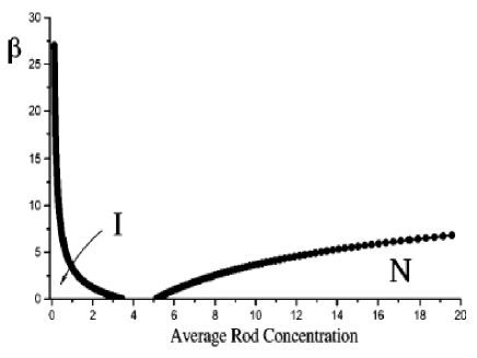
Figure 1: Phase diagram in the variables $\beta$ – $C$ for athermal solution of long rigid rods. Here $\beta\equiv mgh/kT$ is the dimensionless parameter associated with external field, $C$ is the dimensionless average rod concentration. Label $N$ designates the nematic phase, $I$ the isotropic phase while $N+I$ corresponds to phase separation region.

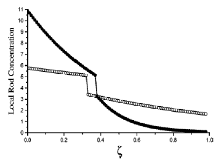
Figure 2: Dependence of the dimensionsless local rod concentration $C(\zeta)$ on the dimensionless height $\zeta$ at fixed value of $\beta$. Open circles correspond to $\beta=1.1$; solid circles correspond to $\beta=6.1$; dimensionless total rod concentration is $C=3.4$.

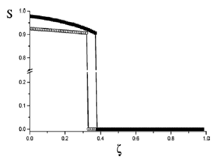
Figure 3: Dependence of the order parameter $S$ on the dimensionless height $\zeta$ at fixed values of $\beta$. Open circles correspond to $\beta=1.1$; solid circles correspond to $\beta=6.1$; dimensionless total rod concentration is $C=3.4$.

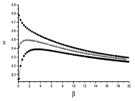
Figure 4: The phase boundary position plotted as a function of $\beta$ for different values of dimensionless total rod concentration $C$. The solid circles refer to $C=4.8$; the open triangles to $C=4.1$; the solid squares to $C=3.4$.

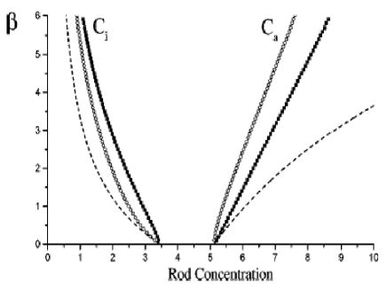
Figure 5: Average concentrations of rods in isotropic and nematic phases as a function of $\beta$ for different values of total rod concentration $C$. Open circles correspond to $C=3.4$, solid squares correspond to $C=4.8$.

- (1) Onsager L. // Ann. N. Y. Acad. Sci. 1949, V. 51, P. 627.
- (2) Flory P. J. // Proc. Roy. Soc. 1956, V. 234, P. 73.
- (3) Fraden S., Maret G., Gaspar D. L. D, Meyer R. // Phys. Rev. Let., 1989. V. 63, P. 2068.
- (4) Fraden S., Maret G., Gaspar D. L. D. // Phys. Rev. E, 1993, V. 48, P. 2816.
- (5) Nakamura H., Okano K. // Phys. Rev. Let., 1983, V. 50, P. 186.
- (6) Adams M., Fraden S. // Biophysical Journal, 1998, V. 74, P. 669.
- (7) Dogic Z., Fraden S. // Phys. Rev. Let., 1997, V. 78, P. 2417.
- (8) Starley J. P. // Mol. Cryst. Liq. Cryst, 1973, V. 22, P. 33.
- (9) Odijk T. // Macromolecules, 1986. V.19, P. 2313.
- (10) Kayser R. F., Raveche H. J. // Phys. Rev. A., 1978, V. 41, P. 53.
- (11) Lekkerkerker H. N. W., Coulon P., van der Haegen R., Deblieck R. // J. Chem. Phys., 1984, V. 80, P. 3427.
- (12) Parsons J. D. // Phys. Rev. A., 1979, V. 19, P. 1225.
- (13) Lee S. D.// J. Chem. Phys., 1987, V. 87, P. 4972.
- (14) Hentschke R.// Macromolecules, 1990, V. 23, P. 1192.
- (15) Pre Du., Yang Y. // J. Chem. Phys., 1991, V. 94, P. 7466.
- (16) Chen J.// Macromolecules, 1993, V. 26, P. 3419.