Wide angle near-field diffraction and Wigner distribution

Abstract

Free-space propagation can be described as a shearing of the Wigner distribution function in the spatial coordinate; this shearing is linear in paraxial approximation but assumes a more complex shape for wide-angle propagation. Integration in the frequency domain allows the determination of near-field diffraction, leading to the well known Fresnel diffraction when small angles are considered and allowing exact prediction of wide-angle diffraction. The authors use this technique to demonstrate evanescent wave formation and diffraction elimination for very small apertures.

The Wigner distribution function (WDF) provides a convenient way to describe an optical signal in space and spatial frequency [1, 2]. The propagation of an optical signal through first-order optical systems is well described by the WDF transformations [3, 4], which allows the reconstruction of the propagated signal. On the other hand, some authors have linked Fresnel diffraction and the fractional Fourier transform (FRFT) [5, 6]; both of these papers associate free-space propagation to a rotation of the WDF and the corresponding FRFT accompanied by a quadratic phase factor.

In this paper we show that free-space propagation is always associated with shearing of the WDF. This can be used to evaluate the near-field diffraction. In the paraxial approximation our results duplicate the well known Fresnel diffraction, with the advantage that we do not need to resort to the Cornu integrals. The same procedure can be extended to wide angles, where other phenomena are apparent, namely the presence of evanescent waves.

The Wigner distribution function (WDF) of a scalar, time harmonic, and coherent field distribution $\varphi(\mathbf{q},z)$ can be defined at a $z=\mathrm{const.}$ plane in terms of either the field distribution or its Fourier transform $\overline{\varphi}(\mathbf{p})=\int\varphi(\mathbf{q})\exp(-ik\mathbf{q}^{T}\mathbf{p})d\mathbf{q}$ [2, 3]:

$$W(\mathbf{q},\mathbf{p}) = \int\varphi\left(\mathbf{q}+\frac{\mathbf{q}^{\prime}}{2}\right)\varphi^{*}\left(\mathbf{q}-\frac{\mathbf{q}^{\prime}}{2}\right)\exp\left(-ik\mathbf{q}^{\prime T}\mathbf{p}\right)d\mathbf{q}^{\prime}$$ (1)

$$= \frac{k^{2}}{4\pi^{2}}\int\overline{\varphi}\left(\mathbf{p}+\frac{\mathbf{p}^{\prime}}{2}\right)\overline{\varphi}^{*}\left(\mathbf{p}-\frac{\mathbf{p}^{\prime}}{2}\right)\exp\left(ik\mathbf{q}^{T}\mathbf{p}^{\prime}\right)d\mathbf{p}^{\prime}~{},$$ (2)

where $\mathbf{q}$ is the position vector, $\mathbf{p}$ the conjugate momentum, $k=2\pi/\lambda$ and ^∗ indicates complex conjugate.

In the paraxial approximation, propagation in a homogeneous medium of refractive index $n$ produces a perfect mapping of the WDF according to the relation [2, 3]

$$W(\mathbf{q},\mathbf{p},z)=W(\mathbf{q}-\frac{z}{n}\mathbf{p},\mathbf{p},0).$$ (3)

After the WDF has been propagated over a distance, the field distribution can be recovered by [2]

$$\varphi(\mathbf{q},z)\varphi^{*}(0,z)=\frac{1}{4\pi^{2}}\int W(\mathbf{q}/2,\mathbf{p},z)\exp(i\mathbf{q}\mathbf{p})d\mathbf{p}.$$ (4)

The field intensity distribution can also be found by

$$|\varphi(\mathbf{q},z)|^{2}=\frac{4\pi^{2}}{k^{2}}\int W(\mathbf{q},\mathbf{p},z)d\mathbf{p}.$$ (5)

Eqs. (4) and (5) are all that is needed for the evaluation of Fresnel diffraction fields. Consider the diffraction pattern for a rectangular aperture in one dimension. The WDF of the aperture is given by

$$W(q,p)=\left\{\begin{array}[]{lc}0&~{}~{}|q|\geq l/2\\ 2\sin[kp(l-2q)]/kp&~{}~{}0\leq q<l/2\\ 2\sin[kp(l+2q)]/kp&~{}~{}-l/2\leq q\leq 0\end{array}\right.,$$ (6)

with $l$ being the aperture width. After propagation and integration in $p$ we obtain

$$\frac{k^{2}|\varphi(q,z)|^{2}}{8\pi^{2}} = \int_{n(2q-l)/(2z)}^{nq/z}\frac{1}{kp}\sin[kp(l-2zp/n-2q)]dp$$ (7)

$$+\int^{n(2q+l)/(2z)}_{nq/z}\frac{1}{kp}\sin[kp(l+2zp/n+2q)]dp.$$

Fig. 1 shows a typical diffraction pattern obtained in this way.

For wide angles the WDF can no longer be mapped from the initial to the final planes. It must be born in mind that the components of the conjugate momentum $\mathbf{p}$ correspond to the direction cosines of the propagating direction multiplied by the refractive index; the appropriate transformation is given by [7]

$$W(\mathbf{q},\mathbf{p},z)=\left\{\begin{array}[]{ll}W(\mathbf{q}-z\mathbf{p}/\sqrt{n^{2}-|\mathbf{p}|^{2}},\mathbf{p},0)&~{}~{}|\mathbf{p}|<n\\ 0&~{}~{}\mathrm{otherwise}\end{array}\right..$$ (8)

Eq. (8) shows that only spatial frequencies corresponding to momenta such that $|\mathbf{p}|<n$ can be propagated [8]. In fact $|\mathbf{p}|/n=\sin\alpha$, with $\alpha$ the angle the ray makes with the $z$ axis. It is then obvious that the higher frequencies would correspond to values of $|\sin\alpha|>1$; these frequencies don’t propagate and originate evanescent waves instead, Fig. 2. The net effect on near-field diffraction is that the high-frequency detail near the aperture is quickly reduced.

The field intensity can now be evaluated by the expression

$$\frac{k^{2}|\varphi(q,z)|^{2}}{4\pi^{2}} = \int_{p_{1}}^{p_{0}}{\frac{1}{kp}\sin\left\{kp\left[l-2\left(q-zp/\sqrt{n^{2}-p^{2}}\right)\right]\right\}dp}$$ (9)

$$+\int_{p_{0}}^{p_{2}}{\frac{1}{kp}\sin\left\{kp\left[l+2\left(q-zp/\sqrt{n^{2}-p^{2}}\right)\right]\right\}dp},$$

with

$$p_{0} = nq/\sqrt{q^{2}+z^{2}},$$

$$p_{1} = n(2q-l)/\sqrt{(2q-l)^{2}+4z^{2}},$$

$$p_{2} = n(2q+l)/\sqrt{(2q+l)^{2}+4z^{2}}.$$ (10)

Fig. 3 shows the near-field diffraction pattern when the aperture is exactly one wavelength wide. The situation is such that all the high order maxima of the WDF appear at values of $|p|>1$ and are evanescent, resulting in a field pattern with one small minimum immediately after the aperture, after which the beam takes a quasi-gaussian shape, without further minima. A sub-wavelength resolution would be possible about half a wavelength in front of the aperture, where the field distribution shows a very sharp peak.

We return now to the subject of FRFT to analyze the connection between this and Fresnel diffraction. Being associated with a rotation of the WDF, the FRFT can only represent diffraction if associated with a quadratic phase factor that effectively transforms the rotation in a shearing operation [5]. The implementation of the FRFT needs a combination of paraxial free-space propagation, a thin lens and a magnification telescope [6, 9].

J. B. Almeida wishes to acknowledge the fruitful discussions with P. Andrés, W. Furlan and G. Saavedra at the University of Valencia.

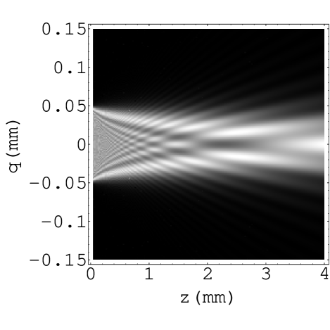
Figure 1: Fresnel diffraction pattern for a one-dimensional aperture of width $0.1~{}\mathrm{mm}$ with $k=10^{7}$.

Figure 2: Propagation of the WDF in wide angle condition ($k=10^{6}~{}\mathrm{m}^{-1}$, horizontal scale in $\mu\mathrm{m}$). a) Original distribution, b) after propagation over $3~{}\mu\mathrm{m}$.

a)
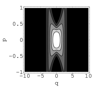
b)

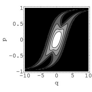
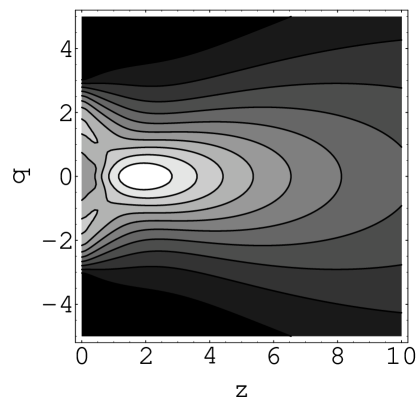
Figure 3: Near-field diffraction pattern when the aperture width is exactly one wavelength; ($k=10^{6}~{}\mathrm{m}^{-1}$, both scales in $\mathrm{\mu m}$).

References

- [1] M. J. Bastiaans, “The Wigner Distribution Function Applied to Optical Signals and Systems,” Opt. Commun. 25, 26–30 (1978).
- [2] D. Dragoman, “The Wigner Distribution Function in Optics and Optoelectronics,” in Progress in Optics, E. Wolf, ed., (Elsevier, Amsterdam, 1997), Vol. 37, Chap. 1, pp. 1–56.
- [3] M. J. Bastiaans, “The Wigner Distribution Function and Hamilton’s Characteristics of a Geometric-Optical System,” Opt. Commun. 30, 321–326 (1979).
- [4] M. J. Bastiaans, “Second-Order Moments of the Wigner Distribution Function in First-Order Optical Systems,” Optik 88, 163–168 (1991).
- [5] T. Alieva, V. Lopez, F. Agullo-Lopez, and L. B. Almeida, “The Fractional Fourier Transform in Optical Propagation Problems,” J. of Modern Optics 41, 1037–1044 (1994).
- [6] G. S. Agarwal and R. Simon, “A Simple Realization of Fractional Fourier Transform and Relation to Harmonic Oscillator Green’s Function,” Opt. Commun. 110, 23–26 (1994).
- [7] K. B. Wolf, M. A. Alonso, and G. W. Forbes, “Wigner Functions for Helmoltz Wave Fields,” J. Opt. Soc. Am. A 16, 2476–2487 (1999).
- [8] J. W. Goodman, Introduction to Fourier Optics (McGraw-Hill, New York, 1968).
- [9] P. Andrés, W. D. Furlan, G. Saavedra, and A. W. Lohman, “Variable Fractional Fourier Processor: A Simple Implementation,” J. Opt. Soc. Am. A 14, 853–858 (1997).
a)
b)