Modeling Stochastic Clonal Interference

Abstract

We study the competition between several advantageous mutants in an asexual population (clonal interference) as a function of the time between the appearance of the mutants $\Delta t$, their selective advantages, and the rate of deleterious mutations. We find that the overall probability of fixation (the probability that at least one of the mutants becomes the ancestor of the entire population) does not depend on the time interval between the appearance of these mutants, and equals the probability that a genotype bearing all of these mutations reaches fixation. This result holds also in the presence of deleterious mutations, and for an arbitrary number of competing mutants. We also show that if mutations interfere, an increase in the mean number of fixation events is associated with a decrease in the expected fitness gain of the population.

1 Introduction

Evolution, according to Dobzhansky (1973), is the unifying concept that pulls together all the different strands of biology. Indeed, while evolution provides the framework to understand the otherwise bewildering panoply of adapted forms, it also allows us to understand the patterns that mutation and selection leave in the molecules of life, namely DNA and proteins. One of the central problems of the branch of biology that is devoted to the systematics of the tree of all living things, molecular evolution, concerns the rate of adaptation of individual organisms and species. A precise understanding of molecular phylogeny requires accurate models of evolution and adaptation. In this contribution, we model the adaptation of chromosomes that do not undergo recombination, or more generally, the rate of adaptation of asexual organisms.

The main observation that we study here is that the rate of adaptation of asexual organisms, or of regions of low recombination in the genomes of sexual organisms, does not steadily increase with increasing rate of advantageous mutations. When two or more advantageous mutations appear in different organisms at approximately the same time, then only one of them can go to fixation, i.e., become shared by all members of the population, while the others will be lost. This loss of potentially beneficial mutations limits the rate of adaptation to the rate at which individual mutants can go to fixation. By contrast, in sexual organisms, several mutations can recombine and thus go to fixation together. This interference of advantageous mutations has long been recognized as a potential disadvantage of asexual populations (Fisher, 1930; Muller, 1964; Hill and Robertson, 1966). Recently, several groups have worked on an exact quantification of the interference effect, both in theoretical studies (Barton, 1995; Gerrish and Lenski, 1998; Orr, 2000; Gerrish, 2001; McVean and Charlesworth, 2000) and in experimental studies with bacteria (de Visser et al., 1999; Rozen et al., 2002; Shaver et al., 2002) and viruses (Miralles et al., 1999; Cuevas et al., 2002). A good quantitative understanding of the interference effect is necessary in order to assess the influence that interference has on the patterns of molecular evolution and variation in large populations.

There are two separate dynamics that both contribute to the overall interference effect: First, if two advantageous mutants are both present in sufficiently high concentrations, such that loss to drift can be neglected, then they compete deterministically, and the mutant with the higher selective advantage will replace the other one. Second, if at least one advantageous mutant is still very rare, then we have to consider the influence of other mutants’ presence on the chance that this mutant is lost to drift. To date, there is no single theory that takes into account both dynamics to their full extent. Gerrish and Lenski (1998) calculated the speed of adaptation as a function of population size and beneficial mutation rate, under the assumption that clonal interference can be neglected during the initial phase of drift. They assumed that the probability that a mutant is not lost to drift corresponds to one minus the standard probability of fixation (as calculated for example by Fisher 1922, Haldane 1927, Kimura 1962) of that mutant. Orr (2000) modified the calculations of Gerrish and Lenski to include beneficial mutations that arise in genomes bearing one or more deleterious mutations, but also did not address the effect of interference of other beneficial mutations during the initial phase of drift. In general, the influence of deleterious mutations on the probability of fixation has been studied extensively (Manning and Thompson, 1984; Charlesworth, 1994; Peck, 1994; Johnson and Barton, 2002), but there are very few studies that consider the effect of interfering beneficial mutations. The problem of interfering advantageous mutations is that there exists no simple theoretical framework with which their influence on drift can be described accurately. Barton (1995) derived an approximation that allowed him to calculate the probability of fixation of a mutant in a population that is undergoing a selective sweep. However, his approximation is valid only for very small selective advantages. McVean and Charlesworth (2000) studied a similar situation with numerical simulations, and applied their results to codon bias and levels of polymorphism in molecular evolution.

Here, we study the mutual interference of two advantageous mutants that are each initially present in only a single organism. We derive a phenomenological description of the mutants’ fixation probabilities in the interference regime. This phenomenological description, which is in essence an interpolation between limiting cases that can be described with standard theory, agrees very well with numerical simulations. We also find that the expected fitness increase of the population is maximized if the mutant with higher selective advantage arrives earlier, even though this order of appearance leads, on average, to fewer mutants that go to fixation.

2 Model

We consider three distinct sequence types: wild type, advantageous mutant 1, and advantageous mutant 2, with fitness values 1, $1+s_{1}$, and $1+s_{2}$, respectively. Thus, $s_{1}$ denotes the selective advantage of mutants of type $1$, and $s_{2}$ is the selective advantage of mutants of type $2$. For simplicity, we assume that $s_{2}>s_{1}$. Initially, the population is homogeneous and consists of the wild type only. Then, one randomly chosen wild type individual is replaced by an advantageous mutant of either type, and some $\Delta t$ generations later, another randomly chosen individual of the population (either wild type or mutant) is replaced by a mutant of the other type. Throughout this paper, we will understand $\Delta t$ to be the difference in generations between the appearance of mutant 2 and mutant 1, so that negative values of $\Delta t$ indicate that mutant 2 appeared before mutant 1.

The population is finite of size $N$, and replication takes place in discrete generations, according to the Wright-Fisher model: All individuals in generation $t$ are direct descendants of the individuals of the previous generation; the probability that an individual is the offspring of a particular parent is proportional to the parent’s fitness. We introduce deleterious mutations into the offspring organisms with probability $u$. If a mutant of type 1 or 2 is hit by a mutation, then its fitness is set to 1 (that is, it reverts to the lower fitness wild type). We do not consider deleterious mutations in the wild type genotype.

We consider a genotype to be fixed if it has become the most-recent common ancestor of the whole population, regardless of whether some individuals in the population have a different genotype. This definition of fixation has been used recently to study fixation of beneficial mutations in a heterogeneous genetic background (Barton, 1995; Johnson and Barton, 2002), and also to investigate the process of fixation in a viral quasispecies (Wilke, 2003).

3 Theoretical analysis

3.1 Probability of ultimate fixation

In the Appendix, we derive equations for the probability of fixation $P(s,u)$ and time to fixation $T(s,u)$ of an individual mutant with selective advantage $s$ and mutation rate $u$. For two mutants, we are mostly interested in the probability of ultimate fixation, that is, the probability that a mutant reaches fixation and is not subsequently replaced by the other mutant. In the following, we will denote the probability that mutant $i$ reaches ultimate fixation under the condition that the two mutants are introduced $\Delta t$ generations apart as $\pi_{i}(\Delta t)$. We can calculate $\pi_{i}(\Delta t)$ for the two limiting cases $\Delta t\rightarrow-\infty$ and $\Delta t\rightarrow\infty$, and present a phenomenological description for intermediate $\Delta t$.

For $\Delta t\rightarrow-\infty$, that is, when mutant 2 arises much earlier than mutant 1, we have

$$\pi_{1}(-\infty) =[1-P(s_{2},u)]P(s_{1},u)\,,$$ (1)

$$\pi_{2}(-\infty) =P(s_{2},u)\,.$$ (2)

Since $s_{2}>s_{1}$, mutant 1 can reach fixation only when mutant 2 has not reached fixation. For $\Delta t\rightarrow\infty$, we have to consider the possibility that mutant 1 reaches fixation first, but is later replaced by mutant 2. Therefore, we find

$$\pi_{1}(\infty) =P(s_{1},u)\Big{[}1-P\Big{(}\frac{1+s_{2}}{(1+s_{1})(1-u)}-1,u\Big{)}\Big{]}\,,$$ (3)

$$\pi_{2}(\infty) =P(s_{1},u)P\Big{(}\frac{1+s_{2}}{(1+s_{1})(1-u)}-1,u\Big{)}+[1-P(s_{1},u)]P(s_{2},u)\,,$$ (4)

where $P(\frac{1+s_{2}}{(1+s_{1})(1-u)}-1,u)$ is the probability that mutant 2 goes to fixation after mutant 1 has already reached fixation. Since $P(\frac{1+s_{2}}{(1+s_{1})(1-u)}-1,u)$ is always smaller than or equal to $P(s_{2},u)$, we have $\pi_{1}(-\infty)\leq\pi_{1}(\infty)$ and $\pi_{2}(-\infty)\geq\pi_{2}(\infty)$. In other words, both mutants have a higher probability of fixation when they are introduced first than when they are introduced second.

For intermediate values of $\Delta t$, there is no theory that enables us to derive a simple expression for $\pi_{i}(\Delta t)$ (but see Barton 1995). We cannot use branching process theory, because it assumes that the presence of the invading mutants does not influence the mean fitness (which they do for intermediate $\Delta t$). Also, diffusion theory becomes unwieldy when there are more than 2 different sequence types. Nevertheless, we have found that we can develop a phenomenological description of the competition of two mutants as follows. We know that $\pi_{i}(t)$ must reach the two limiting values $\pi_{i}(\infty)$ and $\pi_{i}(-\infty)$ for sufficiently large positive or negative $\Delta t$. Moreover, as long as $\Delta t<0$, we do not expect $\pi_{i}(\Delta t)$ to be very different from $\pi_{i}(-\infty)$, because mutant 1 has only a realistic chance of proliferating and going to fixation if mutant 2 is not present in the population. As long as $\Delta t\lesssim 0$, mutant 2 will either go to fixation relatively unscathed from the later appearance of mutant 1, or it will be lost to drift, in which case mutant 1 will have its turn. Likewise, for $\Delta t$ larger than the time to fixation of mutant 1, $T_{1}$, we expect that $\pi_{i}(\Delta t)=\pi_{i}(\infty)$, because $T_{1}$ generations after the introduction of mutant 1, mutant 2 will either find a population in which mutant 1 has already gone to fixation, or one in which it has been lost to drift. For $0\lesssim\Delta t\lesssim T_{1}$, we expect that $\pi_{1}(\Delta t)$ smoothly increases from $\pi_{1}(-\infty)$ to $\pi_{1}(\infty)$, while $\pi_{2}(\Delta t)$ smoothly decreases from $\pi_{2}(-\infty)$ to $\pi_{2}(\infty)$. These considerations suggest a sigmoidal form for $\pi_{i}(\Delta t)$. We use a logistic growth model to describe the smooth transition from $\pi_{i}(-\infty)$ to $\pi_{i}(\infty)$ within the range $0\lesssim\Delta t\lesssim T_{1}$:

$$\pi_{i}(\Delta t)=\pi_{i}(-\infty)+\frac{\pi_{i}(\infty)-\pi_{i}(-\infty)}{1+e^{-\gamma_{1}\left(\Delta t-T_{1}/2\right)}}\;,$$ (5)

where $\gamma_{1}$ is the fitness advantage of mutant 1 at finite mutation rate (see the definition following Eq. (8) below). This expression appears to be an acceptable description of the exact time dependence (see Numerical Results) without free parameters.

3.2 Overall probability of fixation

Besides the individual probabilities $\pi_{1}(\Delta t)$ and $\pi_{2}(\Delta t)$, their sum $\pi=\pi_{1}(\Delta t)+\pi_{2}(\Delta t)$ is also of interest. This sum is the overall probability that at least one mutant goes to fixation. When we sum Eqs. (1) and (2), or Eqs. (3) and (4), we find that the overall fixation probability does not depend on the order in which the mutants are introduced, and has the form

$$\pi=P(s_{1},u)+P(s_{2},u)-P(s_{1},u)P(s_{2},u)\,.$$ (6)

Furthermore, if Eq. (5) is indeed a good description of $\pi_{i}(\Delta t)$ for arbitrary $\Delta t$, then $\pi$ should not depend on $\Delta t$ at all, because all time dependencies cancel when we use Eq. (5) to calculate $\pi_{1}(\Delta t)+\pi_{2}(\Delta t)$.

The invariance of the overall fixation probability $\pi$ under the order by which the mutants appear is a general property. It holds also when more than 2 mutants arise: Assume that $n$ advantageous mutants arise, with selective advantages $s_{1},\dots,s_{n}$ compared to the wild type. Further assume that the time intervals between the appearances of the mutants are large. Then, the probability that none of the mutants make it to fixation is $\prod_{i=1}^{n}[1-P(s_{i},u)]$, regardless of the order of their appearance. The probability that at least one mutant goes to fixation is therefore

$$\pi=1-\prod_{i=1}^{n}[1-P(s_{i},u)]\,,$$ (7)

which reduces to Eq. (6) in the case of $n=2$. Using an extension of Kimura’s well-known result for $P(s_{i},u)$ derived in the Appendix, Eq. (6.4), we can simplify this expression even further. We find in the limit $N\rightarrow\infty$:

$$\pi=1-\exp\left[-2\left(\gamma_{1}+\gamma_{2}+\cdots+\gamma_{n}\right)\right]\,,$$ (8)

with $\gamma_{i}=(1+s_{i})(1-u)-1$ for $u<s_{i}/(1+s_{i})$, and $\gamma_{i}=0$ otherwise. Moreover, in the absence of deleterious mutations, for $u=0$, $\pi$ becomes

$$\pi=1-\exp\left[-2\left(s_{1}+s_{2}+\cdots+s_{n}\right)\right]\,.$$ (9)

In this limit, the overall probability of fixation is the same as the probability of fixation of a single mutant with selective advantage $s$ equal to the sum of the selective advantages of all invading mutants, $s=\sum_{i}s_{i}$. Such a hypothetical mutant is extremely unlikely in clonal populations, because all beneficial mutations would have to hit the lineage sequentially, but could occur when beneficial mutations are shared via recombination. In the limit that all $\gamma_{i}$ vanish (that is, for very large mutation rates or for vanishing $s_{i}$), Eq. (7) becomes

$$\pi=\frac{n}{N}\,.$$ (10)

3.3 Expected fitness increase and expected number of fixed mutants

Depending on which mutant goes to fixation, the average fitness of the final population is either 1, $1+\gamma_{1}$, or $1+\gamma_{2}$, with $\gamma$ as defined following Eq. (8). The expected fitness increase $\langle\gamma(\Delta t)\rangle$ after the introduction of the two mutants is therefore

$$\langle\gamma(\Delta t)\rangle=\gamma_{1}\pi_{1}(\Delta t)+\gamma_{2}\pi_{2}(\Delta t)\,.$$ (11)

Since we know that $\pi_{1}(\Delta t)+\pi_{2}(\Delta t)$ is constant, and $\gamma_{2}\geq\gamma_{1}$ as a direct consequence of our assumption $s_{2}>s_{1}$, it follows that $\langle\gamma(-\infty)\rangle\geq\langle\gamma(\infty)\rangle$. If we write $\pi_{1}(\infty)=\pi_{1}(-\infty)+\Delta\pi$, and $\pi_{2}(-\infty)=\pi_{2}(\infty)+\Delta\pi$, then we find

$$\langle\gamma(-\infty)\rangle-\langle\gamma(\infty)\rangle=(\gamma_{2}-\gamma_{1})\Delta\pi\geq 0\,.$$ (12)

Thus, the expected fitness increase is larger if we introduce the mutant with the higher selective advantage first.

Let $n_{\rm fix}$ denote the number of fixed mutants, that is, we have $n_{\rm fix}=0$ if none of the mutants reach fixation, $n_{\rm fix}=1$ if exactly one of the mutants reaches fixation, and $n_{\rm fix}=2$ if first mutant 1 reaches fixation and is later replaced by mutant 2. For $\Delta t\rightarrow-\infty$ and $N$ large, $n_{\rm fix}$ can never be larger than one, because the probability that mutant 1 goes to fixation in the background of mutant 2 is zero. We find in this limit for the expected value of $n_{\rm fix}$:

$$\langle n_{\rm fix}(-\infty)\rangle=\pi_{1}(-\infty)+\pi_{2}(-\infty)=\pi\,.$$ (13)

In the limit $\Delta t\rightarrow\infty$, on the other hand, we find

$$\langle n_{\rm fix}(\infty)\rangle =\pi_{1}(-\infty)+\pi_{2}(-\infty)+P(s_{1},u)P\Big{(}\frac{1+s_{2}}{(1+s_{1})(1-u)}-1,u\Big{)}$$

$$=\pi+P(s_{1},u)P\Big{(}\frac{1+s_{2}}{(1+s_{1})(1-u)}-1,u\Big{)}\,.$$ (14)

Clearly, $\langle n_{\rm fix}(\infty)\rangle\geq\langle n_{\rm fix}(-\infty)\rangle$. This means that if the mutant with the smaller selective advantage appears before the mutant with the larger selective advantage, then the expected number of mutants that go to fixation is larger than if the mutant with the larger selective advantage appears first. However, at the same time the expected increase in average fitness is smaller, as we saw in the previous paragraph.

4 Numerical Simulation

In order to measure fixation probabilities, we carried out $100,000$ replicates of the simulation for each set of parameters, and recorded the final outcome (all individuals unmarked, or marked as descendants of either advantageous mutant). We studied a population of size $N=1000$ and mutation rates $u=0.0$, 0.01, 0.02, 0.03, 0.05, 0.07, 0.1, 0.15, 0.20, 0.3, 0.4, 0.5, 0.6, 0.7, 0.8. The selective advantages were $s_{1}=0.1$ and $s_{2}=0.2$, $s_{1}=0.1$ and $s_{2}=0.5$, $s_{1}=0.05$ and $s_{2}=0.2$. We also studied a population of size $N=10,000$ for a subset of these parameters, in order to make sure that our results were robust against a change in population size. Because of the sizable amount of CPU time needed to carry out 100,000 replicates for $N=10,000$, we could however not study this case exhaustively.

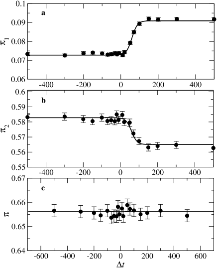
Figure 1: Probability of fixation as a function of time interval $\Delta t$ ($N=1000$, $s_{1}=0.1$, $s_{2}=0.5$, $u=0.0$). Solid lines represent the prediction according to the logistic growth model Eq. (5). a: Probability of fixation of genotype $1$ (less beneficial mutation), $\pi_{1}$. b: Probability of fixation of genotype $2$ (more beneficial mutation), $\pi_{2}$. c: Overall probability of fixation, $\pi$.

In order to keep track of the evolutionary history of each mutant, we marked the initial mutants 1 and 2 with two distinct inheritable neutral markers. In that way, we could distinguish wild type sequences that were descendants from mutants 1 or 2 from the wild type sequences that were originally present. We continued all simulations until all individuals in the population were either unmarked, marked as descendants of mutant 1, or marked as descendants of mutant 2.

Figure 1 shows the probability of ultimate fixation of mutants 1 and 2, $\pi_{1}$ and $\pi_{2}$, and the overall probability of fixation $\pi=\pi_{1}+\pi_{2}$, for $u=0$. We see that the probability $\pi_{1}$ is constant for $\Delta t<0$, and starts to increase as soon as $\Delta t$ turns positive. Eventually, $\pi_{1}$ levels off again. We observe the opposite behavior for the probability $\pi_{2}$. For $\Delta t<0$, $\pi_{2}$ is constant, but decreases rapidly in the same range of $\Delta t$ in which $\pi_{1}$ increases. Finally, $\pi_{2}$ levels off as well.

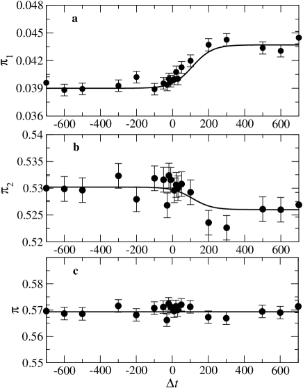
Figure 2: Probability of fixation as a function of time interval $\Delta t$ ($N=1000$, $s_{1}=0.1$, $s_{2}=0.5$, $u=0.05$). Solid lines represent the prediction according to the logistic growth model Eq. (5). a: Probability of fixation of genotype $1$, $\pi_{1}$. b: Probability of fixation of genotype $2$, $\pi_{2}$. c: Overall probability of fixation, $\pi$.

The overall probability of fixation $\pi$ is approximately constant for all values of $\Delta t$. The solid lines in Fig. 1a and b correspond to Eq. (5), and the solid line in Fig. 1c is $\pi_{1}(-\infty)+\pi_{2}(-\infty)$. We find that our phenomenological description Eq. (5) performs very well for intermediate $\Delta t$.

In Fig. 2 we plot the same quantities as those shown in Figure $1$, but now with a positive mutation rate $u=0.05$. We observe that the two probabilities $\pi_{1}$ and $\pi_{2}$ have smaller values than in the absence of mutations. The phenomenological description still works well, and appears to correctly take into account the effects of mutation. The overall fixation probability $\pi$ is again independent of $\Delta t$.

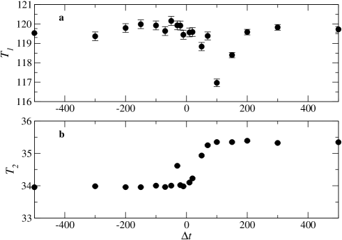
Figure 3: Time to fixation as a function of the time interval between beneficial mutants $\Delta t$ ($N=1000$, $s_{1}=0.1$, $s_{2}=0.5$, $u=0.0$). a: Time to fixation of genotype 1, $T_{1}$. b: Time to fixation of genotype 2, $T_{2}$.

In Figure 3 we show the time to fixation of mutant $1$, $T_{1}$, and the time to fixation of mutant $2$, $T_{2}$, as functions of $\Delta t$. The parameter values are the same as those of Figure 1. In Figure 3a, we see that $T_{1}$ is approximately constant for all values of $\Delta t$ except for the range $0\leq\Delta t\leq 200$. For negative $\Delta t$ the fixation of mutant 1 occurs only when mutant 2 has been eliminated. Therefore, $T_{1}$ corresponds to the result for the fixation time of a mutant with selective advantage $s_{1}$ in a homogeneous population with wild-type individuals only. The same is true for large positive $\Delta t$ because there mutant 1 has enough time to reach fixation without the interference of the second mutant. For small positive $\Delta t$, we observe a decrease of $T_{1}$. The decrease occurs for those $\Delta t$ for which the two beneficial mutants coexist for several generations in the population. Fixation of mutant 1 in this regime occurs only when mutant 1 reaches fixation so quickly that mutant 2 has not had time to build up momentum. Otherwise, most likely mutant 1 will be displaced by mutant 2 before reaching fixation. For mutant 2, the time to fixation $T_{2}$ is shorter for negative $\Delta t$ than for positive $\Delta t$. For positive $\Delta t$, in a fraction of cases mutant 2 has to go to fixation in a background of mutant 1, rather than in a background of wild type. In the background of mutant 1, the selective advantage of mutant 2 is smaller than in a wild-type population, which explains the increased time to fixation. Interestingly, before $T_{2}$ starts to rise for increasing positive $\Delta t$, it quickly spikes at $\Delta t\approx 30$. This spike has the following explanation: If mutant 1 is introduced right before mutant 2 has reached fixation, then the time to fixation of mutant 2 is increased by the additional time it takes for mutant 1 to disappear again. This additional time will typically be one or two generations, which is in agreement with the height of the spike. ($T_{1}$ on the top of the spike is actually approximately half a generation larger than before the spike.) The limiting values for $\pi_{1}$ and $\pi_{2}$ when $\Delta t\rightarrow-\infty$ and $\Delta t\rightarrow-\infty$ were estimated by means of branching process theory which provides very good accuracy, especially for low mutation values.

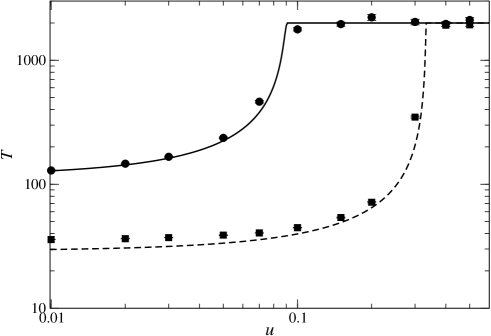
Figure 4: Time to fixation as a function of the mutation probability $u$ ($s_{1}=0.1$ and $s_{2}=0.5$, $\Delta t=100$, $N=1000$). Solid line: the time $T_{1}$ to fixation for the less beneficial mutant, dashed line: time to fixation of more beneficial mutant $T_{2}$.

In Figure 4 we show the fixation times $T_{1}$ and $T_{2}$ as a function of mutation rate obtained from simulations, and compared to the prediction from diffusion theory, Eq. (6.5). As we increase the mutation rate $u$, the population moves from a strong selection regime, characterized by a short time to fixation, to a neutral regime, where $T\approx 2N$. We also observe that the transition between these two regimes occurs at different mutation rates for the two genotypes: $T_{1}$ shows an abrupt transition around the critical value $u=u_{1c}\approx 0.09$, whereas $T_{2}$ reaches the neutral regime around $u=u_{2c}\approx 0.30$. The mutation rate at which this transition occurs is known as the error threshold (Eigen, 1971).

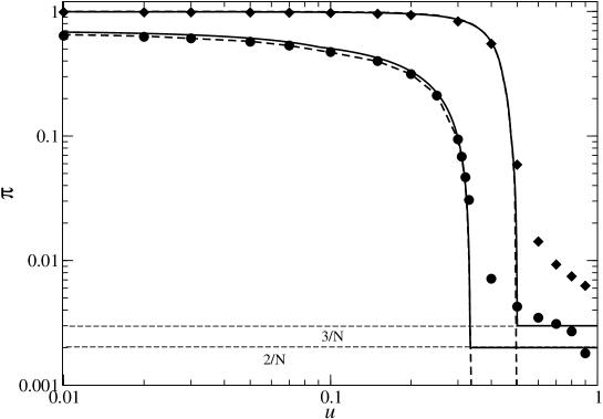
Figure 5: Overall probability of fixation as a function of mutation rate $u$. Circles correspond to the situation of two invading mutants ($s_{1}=0.1$, $s_{2}=0.5$, $\Delta t=100$, $N=1000$), and squares correspond to the situation of three invading mutants ($s_{1}=0.8$, $s_{2}=0.9$, $s_{3}=1.0$, $\Delta t=20$). The solid line is the prediction according to diffusion theory, while the long-dashed line corresponds to the branching process. The short dashes indicate the fixation probability levels according to the neutral theory Eq. (10), for two or three mutants, respectively.

In Figure 5 we can see the overall probability of fixation as a function of mutation rate for the case of two as well as three interfering mutants. Simulation results are again compared to the diffusion theory result Eq. (6.4), but also to a prediction from branching process theory, Eq. (6.14). For these simulations, we used $s_{1}=0.1$, $s_{2}=0.5$ and population size $N=1000$. We also chose a time interval $\Delta t=100$, which is smaller than the time required for fixation of mutant $1$, to ensure that the dynamics takes place in the clonal interference regime. Above the error threshold, the probability of fixation is known to be $1/N$ for a single mutation ($2/N$ and $3/N$ for two or three mutants, respectively). Because the branching process description assumes infinite population size, it predicts zero probability of fixation above the error threshold. Diffusion theory, on the other hand, describes this regime adequately, while being less accurate at small mutation rates. The abrupt change between the ordered and disordered regime predicted by both theories is not present in the numerical data because the simulated system is finite.

Finally, we tested the prediction that the mean number of fixations in the population is larger when the mutant with the smaller selective advantage is introduced first, even though the mean fitness increase is smaller. Figure 6a shows the results for the expected increase in fitness as a function of the time interval $\Delta t$ as defined in Eq. (11), as well as the solution of Eq. (11) using a sigmoidal ansatz for the probabilities $\pi_{1}$ and $\pi_{2}$, as defined in Eq. (5). As expected, the mean fitness gain decreases as $\Delta t$ turns positive, while the expected number of fixed mutants, shown in Figure 6b, increases.

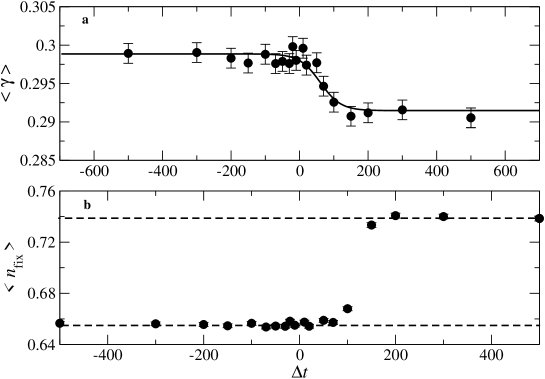
Figure 6: a: Expected increase in fitness due to introduction of mutants as a function of time between their introduction. b: Expected number of fixed mutants (panel b) as a function of $\Delta t$ ($s_{1}=0.1$, $s_{2}=0.5$, $u=0.0$, $N=1000$, for a and batt). Solid line in panel (a) is expected result according to fixation probabilities given by Eq. (5).

5 Discussion

The rate of adaptation of a non-recombining chromosome or asexual population is a non-trivial quantity that depends on details of the fitness distribution of mutations. Beneficial mutations often take a long time to dominate in a population, and compete against each other in the background of deleterious mutations. The probability of fixation of any one mutation depends on the time of their introduction, stochastic drift, and the prevalent mutation rate. A good understanding of the rate of adaptation of asexuals is important in molecular phylogeny, because it influences the speed of the assumed molecular clock (Kuhner and Felsenstein, 1994). Since successive fixation events determine the branchings in the phylogenetic tree, a stochastic analysis of the fixation probability of competing mutations can provide insight into models of evolution used for tree reconstruction methods (Page and Holmes, 1998).

We studied the probability of fixation of beneficial mutations in the presence of other beneficial mutations that were introduced either earlier or later, and in the presence of other deleterious mutations, that is, we studied fixation in a non-equilibrium background. This problem has been addressed previously by Barton (1995) using a deterministic approach, which was unfortunately limited to small selective advantages. Similarly, Johnson and Barton (2002) studied the probability of fixation in a changing background, but they confined themselves mostly to the case where deleterious mutations accumulate in the background after a selective sweep.

We found that the probability of fixation is easily understood from an analytic point of view as long as the time interval between the introduction of mutants is larger than the fixation time of the least beneficial mutation. In the interference regime, where the population consists of clones of the wild type as well as both beneficial mutants, a phenomenological approach based on logistic growth is successful at describing the competition. In general, we find that the probability of fixation of the most beneficial mutant is reduced when it competes against a less beneficial mutant, and there is a sizable probability that the less beneficial mutant will in fact survive (see Fig. 1). Yet, the probability that either one of the mutants survives does not depend on the timing of their introduction.

A number of authors noted the reduction of fixation probabilities caused by segregating deleterious mutations (Peck, 1994; Manning and Thompson, 1984; Charlesworth, 1994; Orr, 2000; Johnson and Barton, 2002), and we observe the same qualitative behavior here. We find that a background of deleterious mutations suppresses the fixation probability, and this suppression is more pronounced for the less beneficial mutant. In the model presented here, there is a simple relationship between beneficial and deleterious mutations: Each mutation occurring on a clone created by a beneficial mutation is reduced to the wild type fitness. This simplified model corresponds to a single-peak landscape, exhaustively studied in the context of quasispecies theory (Tarazona, 1992; Swetina and Schuster, 1982; Galluccio, 1997; Campos and Fontanari, 1998). Consequently, we expect a more pronounced decrease of the probability of fixation for small $s$ due to the existence of an error-threshold, i.e., a point at which information is lost from the sequence due to a critically high mutation rate, see Eigen (1971). In the stochastic regime of evolution, which occurs for mutation rates above the error threshold, individuals replicate randomly, and each member of the population is expected to be the most recent ancestor of the population with the same probability $\pi=1/N$ while the time to fixation is $T=2N$ (Kimura, 1968; Kingman, 1982; Donnelly and Tavaré, 1995). This prediction is confirmed in Figure 4, where we see that for large $u$ both $T_{1}$ and $T_{2}$ are approximately equal to $2N$. Accordingly, in the interval $u_{1c}<u<u_{2c}$, where $u_{ic}$ denotes the error-threshold for genotype of type $i$, we can describe the dynamics by ignoring the less beneficial mutant.

The explicit modeling of stochastic interference between beneficial mutation revealed an interesting observation concerning the mean number of fixation events and the expected fitness change. Naively one might surmise that, as the number of fixation events increases, so does the expected increase in fitness. Instead, we found the opposite dynamic: Fig. 6 clearly shows that if the mutant with the smaller selective advantage appears first, then we expect more fixation events because the second mutant then has a good chance to survive. Yet, this is not the best scenario if we are interested in maximizing fitness: In this case, it is better if the most beneficial mutant can establish itself first, even though this implies that there is little chance for another fixation event.

Finally, we observed that the probability for any beneficial mutant to go to fixation is equal to the probability that a genotype bearing all mutations will become the ancestor of the entire population. Moreover, this observation holds for an arbitrary number of competing mutations, even in the presence of deleterious mutations, independently of the order of appearance of the beneficial mutations. Naturally, while such a probability is very high if the sum of all benefits is large, the probability of a single sequence appearing with this combination of mutations is exponentially small in non-recombining populations. This result was confirmed using an extension of Kimura’s result (1962) to finite mutation rates [Eq. (6.4)] and also by means of a branching process formulation. Both approaches yield similar results and are in excellent agreement with our numerical simulations. We find that the branching process approach is more accurate at low mutation rates, away from the error threshold. As it is formulated in the $N\rightarrow\infty$ limit, it fails to predict the asymptotic result $\pi\approx n/N$ which is reached in the limit that all $\gamma_{i}$ vanish.

The present analysis concerns the rate of adaptation as beneficial mutations compete against each other in the presence of deleterious mutations, in a non-equilibrium framework. This is a step towards the goal of characterizing the rate of adaptation of whole populations in arbitrary circumstances, and in the presence of recombination. We expect that these extensions are necessary before accurate predictions of optimal mutation rates in biological evolution can be made.

6 Probability of fixation and time to fixation for an individual mutant

We can calculate the probability of fixation of an individual mutant either from branching process theory (Fisher, 1922; Haldane, 1927; Fisher, 1930; Barton, 1995; Johnson and Barton, 2002; Wilke, 2003) or from diffusion theory (Kimura, 1962). Branching process theory is applicable for very large population sizes, and arbitrary (but positive) selective advantages $s$. Diffusion theory is applicable to moderately large to large population sizes and small or even vanishing selective advantages $s$. Moreover, diffusion theory also gives an expression for the expected time to fixation.

6.1 Diffusion theory

If the advantageous mutant suffers additional mutations while it goes to fixation, then we typically have to use multi-dimensional diffusion equations, which can be very unwieldy. However, in the simple case treating the advantageous mutant and the wild type only, and where the only effect of deleterious mutations is to revert the advantageous mutant back to wild type, one-dimensional diffusion theory, as developed by Kimura (1962); Kimura and Ohta (1969), is still applicable, and gives satisfying results (van Nimwegen et al., 1999; Wilke et al., 2001).

The main quantities in diffusion theory are the mean $M_{\delta x}$ and the variance $V_{\delta x}$ in the rate of change per generation of the concentration $x$ of the invading mutant. The derivation of these quantities is straightforward (Ewens, 1979), and we find

$$M_{\delta x} =\gamma x(1-x)\,,$$ (6.1)

$$V_{\delta x} =x(1-x)/N\,$$ (6.2)

to first order in $1/N$ and $\gamma$. Here, $\gamma$ is the relative difference in mean fitness between a wild-type population and a population with fixed advantageous mutant. The only difference between these expressions and those of Kimura (1962) is that $\gamma$ replaces the selective advantage $s$ in $M_{\delta x}$. Without mutations ($u=0$), $\gamma$ is equal to $s$, and we recover the standard results. For positive $u$, $\gamma$ has the form

$$\gamma=\left\{\begin{matrix}(1+s)(1-u)-1&\mbox{for $u<s/(1+s)$,}\\ 0&\mbox{for $u\geq s/(1+s)$.}\end{matrix}\right.$$ (6.3)

The mutation rate $u_{\rm c}$ at which $\gamma$ reaches 0, $u_{\rm c}=s/(1+s)$, corresponds to the error threshold of quasispecies theory (Swetina and Schuster, 1982; Eigen et al., 1988, 1989). For mutation rates larger than $u_{\rm c}$, the invading mutant does not have an advantage over the wild type, and the fixation process corresponds to that of a neutral mutant.

The probability of fixation follows now from Kimura (1962) as

$$P(s,u)=\frac{1-e^{-2\gamma}}{1-e^{-2\gamma N}}\,.$$ (6.4)

Likewise, the expected time to fixation follows from Kimura and Ohta (1969) as

$$T(s,u)=J_{1}+\frac{1-P(s,u)}{P(s,u)}J_{2}\,,$$ (6.5)

where

$$J_{1} =\frac{1}{\gamma(1-e^{-2\gamma N})}\int_{1/N}^{1}\frac{(e^{2\gamma Nx}-1)(e^{-2\gamma Nx}-e^{-2\gamma N})}{x(1-x)}dx\,,$$ (6.6)

$$J_{2} =\frac{1}{\gamma(1-e^{-2\gamma N})}\int_{0}^{1/N}\frac{(e^{2\gamma Nx}-1)(1-e^{-2\gamma Nx})}{x(1-x)}dx\,.$$ (6.7)

6.2 Branching process theory

According to Barton (1995), the probability that a beneficial mutation reaches fixation in a genotype with genetic background $i$ follows from iterating the following set of equations:

$$(1-P_{i,t-1})=\sum_{j=0}^{\infty}W_{i,j}(1-P_{i,t}^{*})^{j}\,,$$ (6.8)

where $P_{i,t}$ is the probability of fixation of an allele that is present in a single copy in site $i$ in generation $t$, $W_{i,j}$ denotes the probability that an allele in site $i$ contributes with $j$ offsprings to the next generation, and

$$P_{i,t}^{*}=\sum_{k}M_{i,k}P_{k,t}$$ (6.9)

is the probability that an allele in background $i$ at time $t-1$ would be fixed, given that at time t it is passed to one offspring. The quantity $M_{j,k}$ gives the probability that an offspring from a parent at background $i$ will be at background $k$. If the distribution of offspring is given by a Poisson distribution with mean $(1+s_{i})$, i.e.,

$$W_{i,j}=\frac{(1+s_{i})^{j}}{j!}e^{-(1+s_{i})},$$ (6.10)

then Eq. (6.8) becomes

$$(1-P_{i,t-1})=\exp\left[-(1+s_{i})P_{i,t}^{*}\right].$$ (6.11)

The fixation probabilities correspond to the solution of Eq. (6.8) obtained in the limit $t\rightarrow\infty$.

In our model, we consider only two distinct classes of genotypes, and mutations occur only from advantageous mutant to wild type. Because the wild type has a mean number of offspring per generation exactly equal to $1$, the probability of fixation of wild type sequences in the branching-process formulation vanishes (Harris, 1963). Therefore, the probability of fixation $P(s,u)$ is given by the solution of the equation:

$$P(s,u)=1-\exp\left[-(1+s)(1-u)P(s,u)\right].$$ (6.12)

Unfortunately, it is not possible to derive a closed-form solution to this equation. $P(s,u)$ has to be determined numerically from iterating Eq. (6.12).

Since the relevant parameter seems to be $\gamma=(1+s)(1-u)-1$, the above equation can be written as

$$P(s,u)=1-\exp\left[-(\gamma+1)P(s,u)\right].$$ (6.13)

Although a derivation can not be performed when $n$ beneficial mutants are considered, we found empirically that in this case

$$P(s,u)=1-\exp\left[-\left[\prod_{i=1}^{n}(\gamma_{i}+1)\right]P(s,u)\right].$$ (6.14)

This expression is used to compare numerical results to the branching process theory prediction in Fig. 5.

References

- Barton (1995) Barton, N. H. (1995). Linkage and the limits to natural selection. Genetics 140, 821–841.
- Campos and Fontanari (1998) Campos, P. R. A. and J. F. Fontanari (1998). Finite-size scaling of the quasispecies model. Physical Review E 58, 2664–2667.
- Charlesworth (1994) Charlesworth, B. (1994). The effect of background selection against deleterious mutations on weakly selected, linked variants. Genet. Res. Camb. 63, 213–227.
- Cuevas et al. (2002) Cuevas, J. M., S. F. Elena, and A. Moya (2002). Molecular basis of adaptive convergence in experimental populations of RNA viruses. Genetics 162, 533–542.
- de Visser et al. (1999) de Visser, J. A. G. M., C. W. Zeyl, P. J. Gerrish, J. L. Blanchard, and R. E. Lenski (1999). Diminishing returns from mutation suply rate in asexual populations. Science 283, 404–406.
- Dobzhansky (1973) Dobzhansky, T. (1973). Nothing in biology makes sense except in the light of evolution. The American Biology Teacher 35, 125–129.
- Donnelly and Tavaré (1995) Donnelly, P. and S. Tavaré (1995). Coalescents and genealogical structure under neutrality. Annu. Rev. Genet. 29, 401–421.
- Eigen (1971) Eigen, M. (1971). Selforganization of matter and evolution of biological macromolecules. Naturwissenschaften 58, 465–429.
- Eigen et al. (1988) Eigen, M., J. McCaskill, and P. Schuster (1988). Molecular quasi-species. J. Phys. Chem. 92, 6881–6891.
- Eigen et al. (1989) Eigen, M., J. McCaskill, and P. Schuster (1989). The molecular quasi-species. Adv. Chem. Phys. 75, 149–263.
- Ewens (1979) Ewens, W. J. (1979). Mathematical Population Genetics. Berlin: Springer.
- Fisher (1922) Fisher, R. A. (1922). On the dominance ratio. Proc. Roy. Soc. Edinb. Sect. B Biol. Sci. 42, 321–341.
- Fisher (1930) Fisher, R. A. (1930). The Genetical Theory of Natural Selection. Claredon Press.
- Galluccio (1997) Galluccio, S. (1997). Exact solution of the quasispecies model in a sharply peaked fitness landscape. Phys. Rev. E 56, 4526–4539.
- Gerrish (2001) Gerrish, P. (2001). The rhythm of microbial adaptation. Nature 413, 299–302.
- Gerrish and Lenski (1998) Gerrish, P. J. and R. E. Lenski (1998). The fate of competing beneficial mutations in an asexual population. Genetica 102/103, 127–144.
- Haldane (1927) Haldane, J. B. S. (1927). A mathematical theory of natural and artificial selection. Part V: Selection and mutation. Proc. Camb. Phil. Soc. 26, 220–230.
- Harris (1963) Harris, T. E. (1963). The Theory of Branching Processes. Springer.
- Hill and Robertson (1966) Hill, W. G. and A. Robertson (1966). The effect of linkage on the limits to artificial selection. Genet. Res. 8, 269–294.
- Johnson and Barton (2002) Johnson, T. and N. H. Barton (2002). The effect of deleterious alleles on adaptation in asexual organisms. Genetics 162, 395–411.
- Kimura (1962) Kimura, M. (1962). On the probability of fixation of mutant genes in a population. Genetics 47, 713–719.
- Kimura (1968) Kimura, M. (1968). Evolutionary rate at the molecular level. Nature 217, 624–626.
- Kimura and Ohta (1969) Kimura, M. and T. Ohta (1969). The average number of generations until fixation of a mutant gene in a finite population. Genetics 61, 763–771.
- Kingman (1982) Kingman, J. F. C. (1982). On the genealogies of large populations. J. Appl. Prob. 19A, 27–43.
- Kuhner and Felsenstein (1994) Kuhner, M. and J. Felsenstein (1994). A simulation comparison of phylogeny algorithms under equal and unequal evolutionary rates. Mol. Biol. Evol. 11, 459–68.
- Manning and Thompson (1984) Manning, J. T. and D. J. Thompson (1984). Muller’s ratchet and the accumulation of favourable mutations. Acta Biotheor. 33, 219–225.
- McVean and Charlesworth (2000) McVean, G. A. T. and B. Charlesworth (2000). The effects of Hill-Robertson interference between weakly selected mutations on patterns of molecular evolution and variation. Genetics 155, 929–944.
- Miralles et al. (1999) Miralles, R., P. J. Gerrish, A. Moya, and S. F. Elena (1999). Clonal interference and the evolution of RNA viruses. Science 285, 1745–1747.
- Muller (1964) Muller, H. J. (1964). The relation of recombination to mutational advance. Mutat. Res. 1, 2–9.
- Orr (2000) Orr, H. A. (2000). The rate of adaptation in asexuals. Genetics 155, 961–968.
- Page and Holmes (1998) Page, R. and L. Holmes (1998). Molecular Evolution: A Phylogenetic Approach. Blackwell Science.
- Peck (1994) Peck, J. R. (1994). A ruby in the rubbish: Beneficial mutations, deleterious mutations and the evolution of sex. Genetics 137, 597–606.
- Rozen et al. (2002) Rozen, D. E., J. A. G. M. de Visser, and P. J. Gerrish (2002). Fitness effects of fixed beneficial mutations in microbial populations. Current Biology 12, 1040–1045.
- Shaver et al. (2002) Shaver, A. C., P. G. Dombrowski, J. Y. Sweeney, T. Treis, R. M. Zappala, and P. D. Sniegowski (2002). Fitness evolution and the rise of mutator alleles in experimental Escherichia coli populations. Genetics 162, 557–566.
- Swetina and Schuster (1982) Swetina, J. and P. Schuster (1982). Self-replication with errors: A model for polynucleotide replication. Biophys. Chem. 16, 329–345.
- Tarazona (1992) Tarazona, P. (1992). Error thresholds for molecular quasi-species as phase-transitions - from simple landscapes to spin-glass models. Physical Review A 45, 6038–6050.
- van Nimwegen et al. (1999) van Nimwegen, E., J. P. Crutchfield, and M. Mitchell (1999). Statistical dynamics of the Royal Road genetic algorithm. Theoretical Computer Science 229, 41–102.
- Wilke (2003) Wilke, C. O. (2003). Probability of fixation of an advantageous mutant in a viral quasispecies. Genetics 162, 467–474.
- Wilke et al. (2001) Wilke, C. O., C. Ronnewinkel, and T. Martinetz (2001). Dynamic fitness landscapes in molecular evolution. Phys. Rep. 349, 395–446.