Stability of Semi-Implicit and Iterative Centred-Implicit Time Discretisations

for Various Equation Systems Used in NWP

(Accepted in Monthly Weather Review)

P. Bénard^∗

^∗ Centre National de Recherches Météorologiques, Météo-France, Toulouse, France

27 March 2003

Corresponding address:

Pierre Bénard

CNRM/GMAP

42, Avenue G. Coriolis

F-31057 TOULOUSE CEDEX

FRANCE

Telephone: +33 (0)5 61 07 84 63

Fax: +33 (0)5 61 07 84 53

e-mail: pierre.benard@meteo.fr

ABSTRACT

The stability of classical semi-implicit scheme, and some more advanced iterative schemes recently proposed for NWP purpose is examined. In all these schemes, the solution of the centred-implicit non-linear equation is approached by an iterative fixed-point algorithm, preconditioned by a simple, constant in time, linear operator. A general methodology for assessing analytically the stability of these schemes on canonical problems for a vertically unbounded atmosphere is presented. The proposed method is valid for all the equation systems usually employed in NWP. However, as in earlier studies, the method can be applied only in simplified meteorological contexts, thus overestimating the actual stability that would occur in more realistic meteorological contexts. The analysis is performed in the spatially-continuous framework, hence allowing to eliminate the spatial-discretisation or the boundary conditions as possible causes of the fundamental instabilities linked to the time-scheme itself. The general method is then shown concretely to apply to various time-discretisation schemes and equation-systems (namely shallow-water, and fully compressible Euler equations). Analytical results found in the literature are recovered from the proposed method, and some original results are presented.

1 Introduction

The classical semi-implicit (SI) technique (Robert et al., 1972) has been widely used in NWP since it provides efficient and simple algorithms, at least for spectral models. This classical SI method requires the definition of a constant in time linear "reference" operator ${\cal L}^{*}$, which usually consists in the linearisation of the original system ${\cal M}$, around a stationary reference-state, noted ${\cal X}^{*}$. For a given state ${\cal X}$ of the atmosphere, the evolution of the system, $(\partial{\cal X}/\partial t)={\cal M}.{\cal X}$, is then time-discretised through:

$$\frac{\delta{\cal X}}{\delta t}=({\cal M}-{\cal L}^{*}).{\cal X}+{\cal L}^{*}.\overline{[\cal X]}^{t}$$ (1)

where $(\delta/\delta t)$ is the discretised time-derivative operator, and $\overline{[\rule[5.69054pt]{5.69054pt}{0.0pt}]}^{t}$ is the implicit-centred temporal average operator. The terms linked to the reference operator ${\cal L}^{*}$ are thus treated in a centred-implicit way, whilst the residual non-linear terms are treated explicitly. For this scheme, there is no formal proof of the stability in real atmospheric conditions, due to the explicit treatment of non-linear residuals. This prompted the authors of pioneering NWP applications of the SI scheme to examine theoretically its stability in idealised contexts.

In a seminal study following this approach, Simmons et al., 1978 (SHB78 hereafter) analysed the stability of the SI scheme for the hydrostatic primitive equations (HPE) system with a Leap-Frog (3-TL hereafter) time-discretisation by considering the linearised equations around a stationary state $\overline{\cal X}$ (referred to as "atmospheric state" hereafter) when the resulting linear "atmospheric" operator $\overline{\cal L}$ deviates from the linear "reference" operator ${\cal L}^{*}$ of the SI scheme, thus generating potentially unstable explicitly-treated residuals.

In the vertically-continuous context they performed a stability analysis valid when the eigenfunctions of $\overline{\cal L}$ and ${\cal L}^{*}$ are identical. They showed that when the atmospheric and reference temperature profiles (respectively $\overline{T}$ and $T^{*}$) are isothermal, the stability of the SI scheme requires:

$$0\leq\overline{T}\leq 2T^{*},$$ (2)

hence $T^{*}$ cannot be chosen arbitrarily for applying the 3-TL SI scheme to the HPE system.

In the finite-difference vertically-discretised context, thew showed that a "vertically-discretised analysis" of stability following the same principle simply resulted in the solution of a standard eigenvalue problem. They found empirically that a large static-stability for the reference-state is necessary to maintain the stability of the scheme for realistic thermal atmospheric profiles. As a consequence, they recommended to use a warm isothermal state as reference-state, a rule which was then widely adopted for NWP applications using SI schemes.

Finally, they examined the effect of applying a second-order time-filter in the temporal average of linear terms, and found that an improved stability is obtained, but at the expense of an increased misrepresentation of the wave propagation.

Côté et al., 1983 (CBS83 hereafter), still in the HPE context, examined the stability of the 3-TL SI scheme for a finite-element vertical discretisation using the above vertically-discretised analysis method. They established a stability criterion for the 3-TL SI scheme in terms of the atmospheric and reference static stabilities ($\overline{\gamma}$ and $\gamma^{*}$ respectively):

$$0\leq\overline{\gamma}\leq 2\gamma^{*},$$ (3)

therefore generalizing (2) to not necessarily isothermal thermal profiles.

Still in the HPE context, Simmons and Temperton, 1997 showed with the same method that extrapolating two-time level (2-TL) schemes have more stringent stability constraints than their 3-TL counterpart. For instance, in the isothermal framework of the SHB78 analysis, the stability of the 2-TL SI scheme requires:

$$0\leq\overline{T}\leq T^{*}.$$ (4)

As a consequence, they recommended to use a warmer reference temperature than in the 3-TL case. ST97 also showed that the 2-TL SI scheme was intrinsically damping when stable, a characteristic which was not present in the 3-TL SI scheme. However, 3-TL schemes require a time-filter to damp the unstable computational modes, and this time-filter also damps the transient physical modes. They argue that all these aspects being considered, the effective damping of 2-TL and 3-TL schemes is of comparable overall intensity. This particular debate will be ignored in this paper, in order to focus on stability aspects only.

The relevance of the SI method for solving numerically the fully compressible Euler Equations (EE) was then advocated (Tanguay et al., 1990), and some numerical models in EE using this technique were effectively developed: Caya and Laprise (1999), presented a model in EE with a 3-TL SI scheme (with a moderate time-decentering first-order accurate in time). Semazzi et al. (1995) and Qian et al. (1998) also showed a model in EE but with a 2-TL SI scheme (with a strong time-filter however). Besides, the need of more robust schemes than the classical SI one for solving the EE system became recognized (e.g. Côté et al. 1998, BHBG95), probably motivated by some pathological behaviours with the classical SI scheme under some circumstances.

Schemes with evolution terms treated in a more centred-implicit way are usually believed to have an increased robustness, hence fulfilling the latter emerging need, and some of them were developed for fine-scale models in the EE system. Bubnová et al., 1995 used a 3-TL scheme in which the leading non-linear terms of the EE system are treated in a centred-implicit way, through a partially iterative method. For a 2-TL scheme, Côté et al, 1998, used a fully iterative method, aiming to treat all the evolution terms of the EE system in a centred-implicit way. Cullen (2000) examined the benefit of using such a fully iterative scheme for the HPE system, arguing that an improved accuracy could be obtained beside the improved stability (this latter being not strictly required however for current HPE applications). As a formal justification, he examined the stability of this iterative scheme for the 2-TL shallow-water (SW) system. The analysis was limited to a scheme called "predictor/corrector", which consists in a single additional iteration after the SI scheme. The salient result was that the additional iteration in the "predictor/corrector" scheme allows to recover a extended range of stability as in (2) instead of (4). In the following, these fully iterative schemes with a more centred-implicit treatment of the evolution terms will be referred to as "iterative centred-implicit" (ICI) schemes.

From the theoretical point of view, the current situation is that no stability analysis has been provided for the EE system with SI scheme, and for ICI schemes with more iterations, stability analyses are available only for the SW system.

Here we present a general method to carry out space-continuous stability analyses of the various time-discretisation schemes mentioned above, for any usual meteorological system of NWP interest (SW, HPE, EE), on canonical problems similar to those examined in SHB78. Some original results concerning the EE system and iterative schemes are presented.

This work may also be viewed as a first theoretical investigation about the suitability of various time-discretisation schemes for solving numerically the EE system.

2 General framework for analyses

The general framework for the stability analyses presented here is basically the same as in most earlier studies: The flow is assumed adiabatic inviscid and frictionless in a non-rotating dry perfect-gas atmosphere with a Cartesian coordinate system. Moreover, the flow is assumed linear around an "atmospheric" basic-state $\overline{\cal X}$. The actual evolution of the atmospheric flow is thus described by $\overline{\cal L}$, the linear-tangent operator to ${\cal M}$ around $\overline{\cal X}$. The atmospheric basic-state $\overline{\cal X}$ is chosen stationary, resting, horizontally homogeneous, and hydrostatically balanced. The governing equation for the flow is then:

$$\frac{\partial{\cal X}^{\prime}}{\partial t}=\overline{\cal L}.{\cal X}^{\prime}$$ (5)

where ${\cal X}^{\prime}={\cal X}-\overline{\cal X}$, and the primes are dropped henceforth for clarity.

Following the usual practice in NWP, the linear operator ${\cal L}^{*}$ in (1) is taken as the tangent-linear operator to ${\cal M}$ around a reference-state ${\cal X}^{*}$ which is also chosen stationary, resting, horizontally homogeneous, and hydrostatically balanced. Since $\overline{\cal X}$ is a resting state, the linear Lagrangian time-derivative coincides with the Eulerian time-derivative, and the LHS operator of (5) hence holds for Eulerian models as well as for semi-Lagrangian models .

3 The class of ICI schemes in the linear framework

In the restricted resting and linear framework of section 2, classical SI schemes as well as the iterative schemes mentioned in the introduction can be gathered in a single class of ICI schemes, differing only by their number of iterations. These ICI scheme are first presented for a 2-TL discretisation. In this case, the fully implicit-centred (FIC) scheme writes:

$$\frac{{\cal X}^{+}-{\cal X}^{0}}{\Delta t}=\frac{\overline{\cal L}.{\cal X}^{+}+\overline{\cal L}.{\cal X}^{0}}{2}$$ (6)

where, according to a standard practice for time-discretised equations, the superscripts "+" and "0" stand for time levels $(t+\Delta t)$ and $t$ respectively. The principle of ICI schemes is to approach the FIC solution by starting from an initial "guess" noted ${\cal X}^{+(0)}$, then iterating the following algorithm:

$$\frac{{\cal X}^{+(n)}-{\cal X}^{0}}{\Delta t} = \frac{\overline{\cal L}.{\cal X}^{+(n-1)}+\overline{\cal L}.{\cal X}^{0}}{2}+\frac{{\cal L}^{*}.{\cal X}^{+(n)}-{\cal L}^{*}.{\cal X}^{+(n-1)}}{2}$$ (7)

$$\equiv \frac{\left(\overline{\cal L}-{\cal L}^{*}\right).{\cal X}^{+(n-1)}+\left(\overline{\cal L}-{\cal L}^{*}\right).{\cal X}^{0}}{2}+\frac{{{\cal L}^{*}}.{\cal X}^{+(n)}+{{\cal L}^{*}}.{\cal X}^{0}}{2}$$ (8)

for $n=1,2,...,N_{\rm iter}$. The ${\cal X}^{+}$ state, valid a $(t+\Delta t)$ is then taken as the last iterated state ${{\cal X}}^{+(N_{\rm iter})}$. An examination of this scheme for a model with a single prognostic variable without spatial dependency shows that it acts as a fixed-point algorithm for solving the implicit non-linear scalar equation $f(x)=x$, by using an estimate ${f^{\prime}}^{*}$ of the derivative $f^{\prime}$ as a preconditioner for convergence. The method converges if $\left|(f^{\prime}-{f^{\prime}}^{*})/{f^{\prime}}^{*}\right|<1$. This is a weaker condition than the one for the classical (i.e. not preconditioned) fixed-point method: $\left|f^{\prime}\right|<1$. The initial guess ${\cal X}^{+(0)}$ is arbitrary in ICI schemes, but choosing an appropriate initial guess may help decreasing the magnitude of the discrepancy between FIC and ICI schemes after a fixed number of iterations.

For 3-TL schemes, the ICI scheme can be defined by:

$$\frac{{\cal X}^{+(n)}-{\cal X}^{-}}{2\Delta t} = \frac{{\overline{\cal L}}.{\cal X}^{+(n-1)}+{\overline{\cal L}}.{\cal X}^{-}}{2}+\frac{{{\cal L}^{*}}.{\cal X}^{+(n)}-{{\cal L}^{*}}.{\cal X}^{+(n-1)}}{2}$$ (9)

$$\equiv \frac{\left(\overline{\cal L}-{\cal L}^{*}\right).{\cal X}^{+(n-1)}+\left(\overline{\cal L}-{\cal L}^{*}\right).{\cal X}^{-}}{2}+\frac{{{\cal L}^{*}}.{\cal X}^{+(n)}+{{\cal L}^{*}}.{\cal X}^{-}}{2}$$ (10)

where the superscript "-" denotes a variable taken at the time-level $(t-\Delta t)$.

Here follows a list of some schemes proposed in the literature, with the corresponding characteristics (${{\cal X}}^{+(0)}$ ,$N_{\rm iter}$), in the restricted framework of section 2:

• Classical 2-TL SI extrapolating scheme: $N_{\rm iter}=1$ and ${{\cal X}}^{+(0)}=(2{\cal X}^{0}-{\cal X}^{-})$.

• 2-TL non-extrapolating SI scheme: $N_{\rm iter}=1$ and ${{\cal X}}^{+(0)}={\cal X}^{0}$. However, this scheme is not used in practice since it is only first-order accurate in time, as mentioned in Cullen (2000).

• "Predictor/corrector" scheme of Cullen (2000): $N_{\rm iter}=2$ and ${{\cal X}}^{+(0)}={\cal X}^{0}$.

• Iterative scheme of Côté et al., 1998: general iterative ICI scheme, but used with $N_{\rm iter}=2$ in practice. The choice of ${{\cal X}}^{+(0)}$ is not explicitly indicated.

• FIC scheme: $N_{\rm iter}=\infty$ (does not depend on the choice of ${{\cal X}}^{+(0)}$). This scheme can not be achieved in practice for numerical models, but it may be useful for theoretical examination of the asymptotic behaviour of the ICI schemes.

For 3-TL discretisations, the SI scheme, which corresponds to an ICI scheme with $N_{\rm iter}=1$ and ${{\cal X}}^{+(0)}=(2{\cal X}^{0}-{\cal X}^{-})$ is the only one to be used in practice. However, iterated 3-TL ICI schemes could be used as well, and the 3-TL FIC scheme is equivalent to a 2-TL FIC scheme with a time-step twice as long.

In the general framework, when ${\cal M}$ is not linear, these various schemes cannot be gathered in the unique formalism (7) or (9).

Addition of a second-order time-filter in the above definitions for 2-TL schemes is straightforward. Two main variants are usually considered, depending on whether the filtering is applied only to the time-averages of linear terms (as in SHB78), or also to the time-averages of non-linear terms, in (8). For instance, in a 2-TL SI scheme, the first variant of the filter consists in replacing ${\cal L}^{*}({\cal X}^{+(n)}+{\cal X}^{0})$ by ${\cal L}^{*}[(1+\kappa){\cal X}^{+(n)}+(1-2\kappa){\cal X}^{0}+\kappa{\cal X}^{-}]$ in (8), where $\kappa$ is a (small) positive parameter, and for the second variant, the same modification is also applied to the first RHS term of (8). The scheme then becomes essentially a 3-TL scheme since information at level ${\cal X}^{-}$ is always used. However, the use of large values of $\kappa$ (e.g. $\kappa=0.5$, which eliminates the ${\cal X}^{0}$ contribution) is known to deteriorate the solution through a spurious damping of transient perturbations (e.g. Hereil and Laprise, 1996).

For 3-TL schemes, second-order time-filters are uneffective, and a first-order accurate time-decentering must be used. This consists in replacing ${\cal L}^{*}({\cal X}^{+(n)}+{\cal X}^{-})$ by ${\cal L}^{*}[(1+\epsilon){\cal X}^{+(n)}+(1-\epsilon){\cal X}^{-}]$ in (10), where $\epsilon$ is a (small) positive parameter. The scheme then ceases to be second-order accurate in time since the time-average is no longer centred in time. This results in a spurious damping of transient perturbations even for moderate values of $\epsilon$ (due to the weaker time-selectivity of the filter $\epsilon$ compared to $\kappa$).

4 Conditions for space-continuous analyses

4.1 Conditions on the upper and lower boundaries

Space-continuous analyses are much easier to carry out when the equation system is defined in the whole unbounded atmosphere, because the expression of the normal modes of the system is more general. The following space-continuous analyses will restrict to this case (although this is not strictly required). For systems in which the vertical direction is represented (e.g. HPE and EE systems), this means that the upper and lower boundary conditions must not appear explicitly in the set of governing equations. However for systems cast in mass-based coordinates [such as HPE system in pressure-based coordinate (e.g. SHB78), and EE system in hydrostatic pressure-based coordinate (Laprise, 1992, L92 hereafter)], the upper and lower boundary conditions actually appear inside the set of equations through vertical integral operators with definite bounds at the boundaries of the vertical domain. When they are present, it is assumed that these integral operators can be eliminated, i.e. that $\overline{\cal L}$, ${\cal L}^{*}$ can be transformed to "unbounded" operators by application of appropriate vertical linear differential operators to the prognostic equations which originally involve integral operators, in order that e.g. (5) rewrites as:

$$\frac{\partial}{\partial t}\left(\begin{array}[]{c}l_{1}{\cal X}_{1}\\ \vdots\\ l_{P}{\cal X}_{P}\end{array}\right)=\left(\begin{array}[]{ccc}l_{1}\overline{\cal L}_{11}&\cdots&l_{P}\overline{\cal L}_{1P}\\ \vdots&\ddots&\vdots\\ l_{1}\overline{\cal L}_{P1}&\cdots&l_{P}\overline{\cal L}_{PP}\end{array}\right).\left(\begin{array}[]{c}{\cal X}_{1}\\ \vdots\\ {\cal X}_{P}\end{array}\right)$$ (11)

where $P$ is the number of prognostic variables of the unbounded system, $(l_{1},\ldots,l_{P})$ are linear vertical operators, and $(l_{1}\overline{\cal L}_{11},\ldots,l_{P}\overline{\cal L}_{PP})$ are linear spatial operators which no longer contain any reference to the upper and lower boundaries. The transformed system obtained for $\overline{\cal L}$ can then be written as:

$$\frac{\partial l.{\cal X}}{\partial t}=l.\overline{\cal L}.{\cal X}$$ (12)

where $l$ is the diagonal matrix $(l_{1},\ldots,l_{P})$. A similar condition must be true for ${\cal L}^{*}$ as well: it is assumed that applying the same operator $l$ to ${\cal L}^{*}$ leads to an operator $l{\cal L}^{*}$ for which $l_{i}{\cal L}^{*}_{ij}$ does not contain any reference to the upper and lower boundaries for $(i,\;j)\;\in(1,\ldots,P)$. The first condition for the following analyses is:

• [C1]: There exists a linear operator $l$ such as $l\overline{\cal L}$ and $l{\cal L}^{*}$ have no reference to the upper and lower boundaries.

The system (12) is henceforth referred to as the "unbounded" system.

4.2 Conditions on the stability of the $\overline{\cal X}$ state

The aim of these analyses is to determine in which conditions a stationary state $\overline{\cal X}$ for $l\overline{\cal L}$ will remain a stable equilibrium-state in the time-discretised context, provided it is a stable equilibrium-state in the time-continuous context. Hence the analyses will be restricted to stationary states $\overline{\cal X}$ which are in stable equilibrium. Given the linear context used here, a physical transposition of this condition is:

• [C2]: For any perturbation ${\cal X}(t=0)$ around $\overline{\cal X}$ with a bounded energy-density, the time-evolution ${\cal X}(t)$ resulting from (12) must have a bounded energy-density.

The condition is formulated with energy-density instead of total energy because the domain is unbounded in space. The complex eigenmodes of the unbounded system (12) are the complex functions of space ${\cal X}({\bf r})$ which satisfy:

$$l\overline{\cal L}{\cal X}({\bf r})=\overline{\lambda}l{\cal X}({\bf r})$$ (13)

where $\overline{\lambda}\in{\rm\,\rule[0.28453pt]{0.19919pt}{7.11317pt}\!\!\!\;C}$ and ${\bf r}$ denotes the spatial dependency. The time-evolution of the mode is bounded in time if $\overline{\lambda}$ is a pure imaginary number, and ${\cal X}({\bf r})$ is then a "normal mode" in the usual terminology. Theoretical arguments out of the scope of this paper show that a mathematical transposition of [C2] writes:

• [C2’]: For any complex eigenmode of $l\overline{\cal L}$, $\;\;\overline{\lambda}\in i{\rm I\!\!\!\;R}\;\Longleftrightarrow\;{\cal X}({\bf r})$ has a bounded energy-density.

4.3 Conditions on the normal modes of the linear unbounded system

The time-continuous normal modes of the original system (5) are the complex functions of space ${\cal X}({\bf r})$ which have an oscillatory temporal evolution. Hence they satisfy $\overline{\cal L}{\cal X}({\bf r})=i\,\overline{\omega}{\cal X}({\bf r})$. Similarly, the time-continuous normal modes of the linear unbounded system (12) are the complex functions of space ${\cal X}({\bf r})$ for which $l{\cal X}({\bf r})$ has an oscillatory temporal evolution. Hence they satisfy $l.\overline{\cal L}{\cal X}({\bf r})=i\,\overline{\omega}l.{\cal X}({\bf r})$.

Any normal mode of the original system is also necessarily a normal mode of the unbounded system, with the same frequency $\overline{\omega}$. For any normal mode of the unbounded system , we can choose the origin of space o in such a way that this mode writes:

$${\cal X}({\bf r})={\cal X}({\bf o})f({\bf r})=\widehat{\cal X}f({\bf r})$$ (14)

with $\widehat{\cal X}=(\widehat{\cal X}_{1},\ldots,\widehat{\cal X}_{P})\in{\rm\,\rule[0.28453pt]{0.19919pt}{7.11317pt}\!\!\!\;C}^{P}$, and $f=(f_{1},\ldots,f_{P})$ is a vector of space-dependent functions (the product $\widehat{\cal X}f\;$ is understood "component by component"). For the indices $i$ such as ${\cal X}_{i}$ uniformly vanishes, $\widehat{\cal X}_{i}=0$ and $f_{i}({\bf r})=1$ are assumed by convention. The function $f$ and the vector $\widehat{\cal X}$ are respectively termed the "structure" and the "polarisation vector" of the mode. The two following conditions are required for the proposed analyses:

• [C3]: For any normal mode ${\cal X}$ of the unbounded linear atmospheric system with a structure $f({\bf r})$, $\;l_{i}.f_{i}({\bf r})$ must be proportional to $f_{i}({\bf r})$:

$$\forall i\in(1,\ldots,P){\rm\;,\;\;}l_{i}f_{i}({\bf r})=\xi_{i}f_{i}({\bf r}){\rm\;\;with\;}\xi_{i}\in{\rm\,\rule[0.28453pt]{0.19919pt}{7.11317pt}\!\!\!\;C}^{*}.$$ (15)

and:

• [C4]: For any normal mode ${\cal X}$ of the unbounded linear atmospheric system with a structure $f({\bf r})$, $\;\overline{\cal L}_{ij}.f_{j}({\bf r})$ [resp. ${\cal L}^{*}_{ij}.f_{j}({\bf r})$] must be proportional to $f_{i}({\bf r})$:

$$\forall(i,j){\rm,\;\;}l_{i}\overline{\cal L}_{ij}.f_{j}({\bf r})=\overline{\mu}_{ij}f_{i}({\bf r})\;\;{\rm and\;\;}l_{i}{\cal L}^{*}_{ij}.f_{j}({\bf r})=\mu^{*}_{ij}f_{i}({\bf r}){\rm,\;with\;\;}(\overline{\mu}_{ij},\,\mu^{*}_{ij})\;\;{\in}\;\;{\rm\,\rule[0.28453pt]{0.19919pt}{7.11317pt}\!\!\!\;C}.$$ (16)

As will be seen below, these latter two conditions have the important consequence that for any normal mode of the unbounded system, each individual time-discretised prognostic equation for ${\cal X}_{i}({\bf r})$ becomes a scalar equation. This key ingredient makes the analysis straightforward for every member of the ICI class.

4.4 Comments

Since the set of normal modes for the unbounded system encompasses the set of normal mode of the bounded system, the transformation from the bounded system to the unbounded system is not likely to "mask" some instabilities of the original system, unless the causes of the instability lie in the boundary conditions themselves. However, discretised-analyses allow to clarify this point by showing that the stability of the bounded and unbounded systems are actually found to be similar in practice. Besides, discretised-analyses of the unbounded system are by nature impossible to perform, hence the continuous analysis is the only way to estimate the intrinsic stability of the unbounded system and to demonstrate that instabilities, when they occur in a practical application, are not due to a weakness in the spatial discretisation or even to the boundary conditions, but actually to the time-discretised propagation of free modes inside the atmosphere.

In spite of their apparently abstract and constraining form, conditions [C1]–[C4] are easy to verify with routine normal mode analysis techniques when examining a particular concrete meteorological system. The condition [C2’] restricts the set of stationary states $\overline{\cal X}$ around which the analysis is meaningful, and conditions [C1], [C3], [C4] restrict the spectrum of meteorological contexts accessible to the analysis, since they require a qualitative similarity between $l$, $\overline{\cal L}$ and ${\cal L}^{*}$ operators. As stated in SHB78, analyses performed under this type of conditions "…grossly exaggerate the stability of the scheme…" since in more realistic meteorological contexts, the atmospheric and reference operators can be qualitatively much more different than imposed by this condition.

5 Time-Discretised Space-Continuous Analysis

The analysis examine the stability of the time-discretised system for perturbations which have a time-continuous normal mode structure. Hence we consider a given function $f=(f_{1},\ldots,f_{P})$ which is a normal mode structure for the time-continuous system, and we determine the normal modes of the time-discretised system which have the same structure $f$, by solving the equation:

$$\widehat{\cal X}_{(t=\Delta t)}f({\bf r})=\lambda\widehat{\cal X}_{(t=0)}f({\bf r})$$ (17)

where $\widehat{\cal X}_{(t=0)}$ and $\lambda$ are the unknowns, and $\widehat{\cal X}_{(t=\Delta t)}$ is determined using the time-discretisation scheme (7) or (9). For schemes using three time levels (as Leap-Frog or extrapolating 2-TL) a similar relationship $\widehat{\cal X}_{(t=-\Delta t)}f({\bf r})=\lambda^{-1}\widehat{\cal X}_{(t=0)}f({\bf r})$ must be added. If for some solution, $\left|\lambda\right|>1$ (resp. $<1$) the scheme is unstable (resp. damping) for this particular mode. The ratio ${\rm Arg}(\lambda)/(i\overline{\omega}\Delta t)$ gives the relative phase-speed error of the scheme for this mode.

The analysis is described here for a 2-TL discretisation (7), but the transformation to a 3-TL scheme as well as the addition of time-filters such as $\kappa$ or $\epsilon$ are straightforward. In the following of this section, the notation ${\cal X}({\bf r},t)$ is replaced by the usual superscript notation for time-discretised variables ${\cal X}^{t}({\bf r})$ as in section 3.

As a consequence of the discussion in section 3 and applying (17) , ${\cal X}^{+(0)}$ can be written as ${\cal X}^{+(0)}({\bf r})=\mu(\lambda){\cal X}^{0}({\bf r})$, where $\mu(\lambda)$ depends on the choice of the initial guess ${\cal X}^{+(0)}$ (e.g. $\mu=1$ for a 2-TL non-extrapolating scheme, $\mu=2-1/\lambda$ for a 2-TL extrapolating scheme, etc…). The original unbounded system (12) is thus time-discretised following (7):

$$l{\cal X}^{+(0)}({\bf r}) = \mu(\lambda)\,l{\cal X}^{0}({\bf r})$$

$$\frac{{l{\cal X}}^{+(n)}({\bf r})-{l{\cal X}}^{0}({\bf r})}{\Delta t} = \frac{{l\overline{\cal L}}.{{\cal X}}^{+(n-1)}({\bf r})+{l\overline{\cal L}}.{{\cal X}}^{0}({\bf r})}{2}$$

$$+\frac{{l{\cal L}^{*}}.{{\cal X}}^{+(n)}({\bf r})-{l{\cal L}^{*}}.{{\cal X}}^{+(n-1)}({\bf r})}{2}\;,\;\;n\in(1,\ldots,N_{\rm iter})$$

$$l{\cal X}^{+}({\bf r})\equiv l\lambda{\cal X}^{0} = l{\cal X}^{+(N_{\rm iter})}({\bf r})$$

For schemes with $N_{\rm iter}\geq 2$, it is assumed that the intermediate states $l{{\cal X}}^{+(n)}({\bf r})$ for $i\;\in(1,\ldots,N_{\rm iter}-1)$ have the same structure $f$ as the one currently examined, which allows to define the polarisation vector $\widehat{\cal X}_{i}^{+(n)}$ by:

$$l_{i}{\cal X}_{i}^{+(n)}({\bf r})=\widehat{\cal X}_{i}^{+(n)}l_{i}f_{i}({\bf r}).$$ (18)

Hence, using (15) and (16), the space dependency $f_{i}({\bf r})$ eliminates. For the generalized state-vector ${\cal Z}=(\widehat{\cal X}^{0},\widehat{\cal X}^{+(0)},\widehat{\cal X}^{+(1)},\ldots,\widehat{\cal X}^{+(N_{\rm iter})})$ of length $(N_{\rm iter}+2)\times P$, the above system writes:

$$\left(\begin{array}[]{cccccc}\mu(\lambda)I_{P}&-I_{P}&0_{P}&\cdots&\cdots&0_{P}\\ M_{1}&M_{2}&M_{3}&\ddots&&\vdots\\ \vdots&0_{P}&\ddots&\ddots&\ddots&\vdots\\ \vdots&\vdots&\ddots&\ddots&\ddots&0_{P}\\ M_{1}&\vdots&&\ddots&M_{2}&M_{3}\\ -\lambda I_{P}&0_{P}&\cdots&\cdots&0_{P}&I_{P}\end{array}\right).{\cal Z}={\bf M}.{\cal Z}=0.$$ (19)

where $I_{P}$ (resp. $0_{P}$) is the unit (resp. null) $P$-order matrix, and:

$$\left(M_{1}\right)_{ij} = -\delta_{ij}-\frac{\Delta t}{2}\frac{\overline{\mu}_{ij}}{\xi_{i}}$$ (20)

$$\left(M_{2}\right)_{ij} = -\frac{\Delta t}{2}\frac{1}{\xi_{i}}\left(\overline{\mu}_{ij}-\mu^{*}_{ij}\right)$$ (21)

$$\left(M_{3}\right)_{ij} = +\delta_{ij}-\frac{\Delta t}{2}\frac{\mu^{*}_{ij}}{\xi_{i}}$$ (22)

where $\delta_{ij}$ is the $(i,j)$ Kronecker symbol. The possible values of $\lambda$ for the normal mode structure $f({\bf r})$ that we examine, are thus given by the roots of the following polynomial equation in $\lambda$:

$${\rm Det}({\bf M})=0$$ (23)

The dependencies to $\lambda$ are limited to the top- and bottom-left blocks. For a non-extrapolating 2-TL scheme the degree of the polynomial is $P$, and there are $P$ physical modes associated with this structure $f({\bf r})$. For time-schemes making use of three time-levels (i.e. 3-TL schemes, or extrapolating 2-TL schemes, or 2-TL schemes with a time-filter), the degree becomes $2P$, and there are $P$ additional computational modes. The growth-rate for any of these modes is given by the modulus of the corresponding complex root of (23). The growth rate of the time scheme for the considered structure $f$ is then defined by the maximum value of the modulus of these $P$ or $2P$ roots:

$$\Gamma(f)={\rm Max}\left(\left|\lambda_{i}(f)\right|\right),\;\;i\in(1,\ldots,P)\;\;\left[\,{\rm or}\;\;(1,\ldots,2P)\,\right]$$ (24)

Analytical solution of (23) is not possible for large values of $P$, and a numerical solution is often needed.

In this paper we will call "asymptotic growth-rate" the growth-rate for the matrix ${\bf M}$ in the limit of large time-steps $\Delta t\rightarrow\infty$. The analysis of the asymptotic growth-rate is easier than for finite time-steps, since the matrix ${\bf M}$ of (23) degenerates to a matrix ${\bf M^{\prime}}$ in which $\delta_{ij}$ vanishes and $\Delta t/2$ eliminates. Another advantage of asymptotic growth-rates is that they appear to be independent of the structure $f$ in most of the cases examined below, thus simplifying considerably the interpretation of the results. When the asymptotic growth-rate is independent of the structure $f$ the growth-rate of the scheme can be defined by the growth-rate obtained for this scheme with any structure $f$.

When the growth rate for a given scheme is one (or less) for any mode of any normal mode structure $f$, the scheme is then said to be "unconditionally stable" (being understood "in $\Delta t$"). The criterion for unconditional stability obtained through ${\rm Det}({\bf M^{\prime}})=0$ is not only of academic interest since the considered time-schemes are actually used with large time-steps in NWP: the practice shows that a scheme which is not unconditionally stable in the simplified context of these analyses has few chance to be robust enough for use in real conditions.

6 Simple examples: 1D systems

6.1 1D Shallow-water system

The linearised 1D shallow water system in an horizontal direction $x$ can be classically written in terms of the wind $u$ along $x$, and the geopotential $\phi$:

$$\frac{\partial u}{\partial t} = -\frac{\partial\phi}{\partial x}$$ (25)

$$\frac{\partial\phi}{\partial t} = -\overline{\phi}\frac{\partial u}{\partial x}$$ (26)

This system is also valid for the external mode of an isothermal atmosphere in HPE and EE system, replacing $\overline{\phi}$ by $4(R^{2}/C_{p})\overline{T}$ (which is done in the following). The reference system is obtained by replacement of $\overline{T}$ by $T^{*}$, and a "non-linearity" factor is defined through: $\alpha=(\overline{T}-T^{*})/T^{*}$. Solution of (13) implies that if $\overline{T}<0$, $\;\overline{\lambda}\in i{\rm I\!\!\!\;R}\;\Longrightarrow\;u=\widehat{u}\exp(rx)$, which has not a bounded energy-density for $rx\longrightarrow+\infty$. Hence [C2’] requires $\overline{T}\geq 0$ (i.e. $\alpha\geq-1$). The boundary conditions do not appear explicitly in the system, hence $l$ can be taken as the identity operator to satisfy [C1], and [C3]. In the notations of section 4 and 5 we have $P=2$ , ${\cal X}_{1}=u$ and ${\cal X}_{2}=\phi$. The normal modes of the system write $\psi(x)=\widehat{\psi}\exp(ikx)$ with $k\in{\rm I\!\!\!\;R}$ and $\psi=(u,\phi)$. Conditions [C1] – [C4] are easily checked to be satisfied.

For a 3-TL SI scheme, (23) writes:

$$\left(\frac{\lambda^{2}-1}{2\Delta t}\right)^{2}=-\frac{k^{2}c^{*2}}{4}\left(\lambda^{2}+1\right)\left(\lambda^{2}+1+2\alpha\lambda\right),$$ (27)

where $c^{*}=2\sqrt{(R/C_{p})RT^{*}}$. In the limit of long time-steps, the LHS term disappears, and the four roots of the RHS give the "asymptotic" numerical growth-rate for the two physical and two computational modes of the system. The two roots of the first factor have a neutral stability, while those of the second factor have a modulus equal to 1 if $-1\leq\alpha\leq 1$. The criterion (on $\overline{\cal X}$, ${\cal X}^{*}$) for unconditional stability (in $\Delta t$) of the 3-TL SI scheme is thus : $0\leq\overline{T}\leq 2T^{*}$. Some further algebraic manipulations from (23) with $\Delta t=\infty$ show that this criterion remains unchanged when increasing $N_{\rm iter}$.

For a 2-TL SI non-extrapolating ($\mu=1$) scheme, (23) becomes:

$$\left(\frac{\lambda-1}{\Delta t}\right)^{2}=-\frac{k^{2}c^{*2}}{4}\left(\lambda+1\right)\left(\lambda+1+2\alpha\right),$$ (28)

and the criterion for unconditional stability becomes more constraining than for the 3-TL scheme: $-1\leq\alpha\leq 0$ (i.e. $0\leq\overline{T}\leq T^{*}$). The asymptotic growth-rate of a 2-TL non-extrapolating ICI scheme with $N_{\rm iter}$ iterations is given by:

$$\Gamma={\rm Max}\left(1,\left|2(-\alpha)^{N_{\rm iter}}-1\right|\right)$$ (29)

The domain for unconditional stability is thus $-1\leq\alpha\leq 0$ for odd values of $N_{\rm iter}$, and $-1\leq\alpha\leq 1$ for even values of $N_{\rm iter}$.

6.2 1D vertical acoustic system in mass-based coordinate

We consider a vertical 1D compressible atmospheric column satisfying the conditions listed in section 2. A regular mass-based coordinate $\sigma=(\pi/\pi_{s})$ is chosen following L92, by making $\eta=\sigma$, $A(\sigma)=0$ and $B(\sigma)=\sigma$ in equation (31) of L92. The variable $\pi$ denotes the hydrostatic pressure, and $\pi_{s}$, the surface hydrostatic pressure. The system is readily obtained from equations (36) – (45) of L92 by removing all horizontal dependencies. The surface hydrostatic-pressure does not evolve in time (see equation (45) in L92).

The equations are linearised around a resting atmospheric-state $\overline{\cal X}$ and a resting reference-state ${\cal X}^{*}$, both satisfying the conditions of section 2. The temperatures $\overline{T}$ and $T^{*}$ are taken uniform, and we still define the "non-linearity" factor by: $\alpha=(\overline{T}-T^{*})/T^{*}$. The pressure values $\overline{p}$ and $p^{*}$ are assumed to be equal to a common value $\pi_{0}$ at the origin ($\sigma=1$). Since $\overline{\cal X}$ and ${\cal X}^{*}$ are hydrostatically balanced, $\overline{p}=\overline{\pi}=\sigma\pi_{0}$ and $p^{*}=\pi^{*}=\sigma\pi_{0}$ at any level. The thermodynamics equation decouples and the linear system around $\overline{\cal X}$ for the vertical velocity $w$ , and the pressure deviation $p^{\prime}=p-\overline{p}$ writes in standard notations:

$$\frac{\partial w}{\partial t} = \frac{g}{\pi_{0}}\frac{\partial p^{\prime}}{\partial\sigma}$$ (30)

$$\frac{\partial p^{\prime}}{\partial t} = \frac{C_{p}}{C_{v}}\frac{g\pi_{0}}{R\overline{T}}\sigma^{2}\frac{\partial w}{\partial\sigma}$$ (31)

The same derivation holds for ${\cal L}^{*}$ and leads to an operator formally identical to the RHS of (30)-(31), still acting on $(w,p^{\prime})$, but with $\overline{T}$ replaced by $T^{*}$. The solution of (13), implies that if $\overline{T}<0$, $\overline{\lambda}\in\;i{\rm I\!\!\!\;R}\;\Longrightarrow\;w=\widehat{w}\;\sigma^{r}$ with $r<-1$ or $r>0$. For the mode with $r<-1$, the energy-density is not bounded when $\sigma\rightarrow 0$. If $\overline{T}\geq 0$, the structure of the normal modes of (30)-(31) is given by:

$$w(\sigma) = \widehat{w}\;\sigma^{(i\nu-1/2)}=\widehat{w}\;f_{1}(\sigma)$$ (32)

$$p^{\prime}(\sigma) = \widehat{p^{\prime}}\;\sigma^{(i\nu+1/2)}=\widehat{p^{\prime}}\;f_{2}(\sigma)$$ (33)

where $\nu$ is a real number, and they have a bounded energy-density. The condition [C2’] therefore requires $\overline{T}\geq 0$ (i.e. $\alpha\geq-1$). Finally, [C4] is trivially checked to be satisfied.

For a 3-TL SI scheme, (23) writes:

$$\left(\frac{\lambda^{2}-1}{2\Delta t}\right)^{2}=-\frac{(\nu^{2}+1/4)c^{*2}}{4H^{*2}}\left(\lambda^{2}+1\right)\left(\lambda^{2}+1-\frac{2\alpha\lambda}{1+\alpha}\right),$$ (34)

where $c^{*}=\sqrt{(C_{p}/C_{v})RT^{*}}$ and $H^{*}=RT^{*}/g$. Comparison of (34) and (27) shows that the stability of the 1D vertical system for $\alpha$ is the same as the one of the previous shallow-water system for $\alpha^{\prime}=-\alpha/(1+\alpha)$. Hence the criteria for unconditional stability directly follows from those of the previous case, by similarity arguments. The criterion for unconditional stability of the 3-TL SI scheme is $\alpha\geq(-1/2)$, i.e. $\overline{T}\geq(1/2)T^{*}$, and this criterion remains unchanged when increasing $N_{\rm iter}$.

For a 2-TL SI non-extrapolating ($\mu=1$) scheme, (23) becomes:

$$\left(\frac{\lambda-1}{\Delta t}\right)^{2}=-\frac{(\nu^{2}+1/4)c^{*2}}{4H^{*2}}\left(\lambda+1\right)\left(\lambda+1-\frac{2\alpha}{1+\alpha}\right),$$ (35)

and the criterion for unconditional stability ($\alpha\geq 0$, i.e. $\overline{T}\geq T^{*}$), which is more constraining than for the 3-TL SI scheme. For iterated 2-TL schemes, the criterion for unconditional stability is $\alpha\geq(-1/2)$ for even values of $N_{\rm iter}$, and $\alpha\geq 0$ for odd values.

6.3 1D vertical acoustic system in height-based coordinate

In this example we show that the stability properties of the 1D vertical system may depend on the coordinate. The framework is taken as in the previous example except that the vertical coordinate is the height $z$. The linearised system $\overline{\cal L}$ (cf. e.g. Caya and laprise, 1999) writes:

$$\frac{\partial w}{\partial t} = -R\overline{T}\frac{\partial q^{\prime}}{\partial z}+g\frac{T^{\prime}}{\overline{T}}$$ (36)

$$\frac{\partial T^{\prime}}{\partial t} = -\frac{R\overline{T}}{C_{v}}\frac{\partial}{\partial z}w$$ (37)

$$\frac{\partial q^{\prime}}{\partial t} = \left(\frac{g}{R\overline{T}}-\frac{C_{p}}{C_{v}}\frac{\partial}{\partial z}\right)w,$$ (38)

where $q^{\prime}=q-\overline{q}$, $q={\rm ln}(p/p_{0})$, $\overline{q}=-gz/R\overline{T}$, $p_{0}$ is a reference pressure, and $p$ is the true pressure. The normal modes of $\overline{\cal L}$ have the following form, for $\psi=(w,T^{\prime},q^{\prime})$:

$$\psi=\widehat{\psi}\;\exp\left[\left(i\nu+\frac{1}{2\overline{H}}\right)z\right]$$ (39)

where $\overline{H}=(R\overline{T}/g)$. The reference system ${\cal L}^{*}$ is defined in a similar way replacing $\overline{T}$ by $T^{*}$ and $\overline{q}$ by $q^{*}=-gz/RT^{*}$. It should be noted that the structure of the normal modes of ${\cal L}^{*}$ is not the same as for $\overline{\cal L}$ since the characteristic height for ${\cal L}^{*}$ is $H^{*}=(RT^{*}/g)$

For a 2-TL SI non-extrapolating ($\mu=1$) scheme, (23) becomes:

$$\left(\frac{\lambda-1}{\Delta t}\right)^{2}=\frac{c^{*2}}{4}\left(i\nu+\frac{1}{2\overline{H}}\right)\left(\lambda+1+2\alpha\right)\left[i\nu\left(\lambda+1\right)-\frac{1}{H^{*}}\left(\frac{1+2\alpha}{1+\alpha}\right)\left(\lambda+1-\frac{4\alpha}{1+2\alpha}\right)\right]$$ (40)

where $c^{*}=\sqrt{(C_{p}/C_{v})RT^{*}}$. In the height-coordinate framework, the asymptotic growth-rate depends on the structure since $\nu$ appears in one of the factors which become dominant at large time-steps. The interpretation of the results is thus slightly complicated in comparison to the case of a mass-based coordinate. For the most external structure ($\nu=0$), the asymptotic growth-rate is given by the roots of:

$$\left(\lambda+1+2\alpha\right)\left(\lambda+1-\frac{4\alpha}{1+2\alpha}\right)=0.$$ (41)

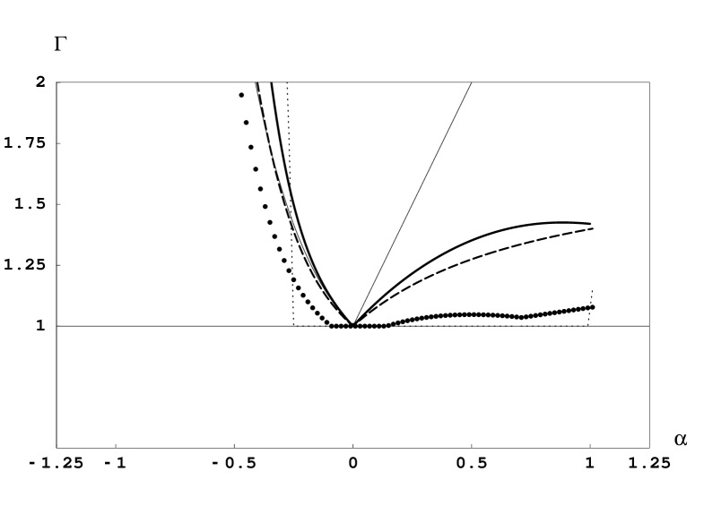
Figure 1: Asymptotic growth-rates $\Gamma$ for 1D vertical system in $z$ coordinate as a function of the nonlinearity parameter $\alpha$. thin line: long mode ($\nu=0.0001\;{\rm m}^{-1}$) with 2-TL SI scheme; thick line: long mode with 2-TL ICI scheme $N_{\rm iter}=2$; dotted line: external mode ($\nu=0$)with 3-TL SI scheme; dashed line: long mode with 3-TL SI scheme. Circles: practical growth-rate of the 3-TL SI scheme for the long mode with $\Delta t=30$ s and $\epsilon=0.1$.

This polynomial consists in a combination of two factors similar to those obtained in the two previous examples (through a formal replacement of $2\alpha$ by $\alpha$ for the second factor). As a consequence, the unconditional stability domains can be readily deduced from these previous examples: the external structure $\nu=0$ is unstable for any value $\alpha\neq 0$ when $\Delta t\longrightarrow\infty$. The instability is thus much more severe than in the case of a mass-based vertical coordinate, for which $\alpha\geq 0$ was sufficient to ensure unconditional stability. Moreover, slightly shorter structures with vertical wavelengths of the order of $(1/\overline{H})$ are found to be more unstable than the external one, and for these structures, the unconditional stability criterion ($\alpha=0$) remains unchanged when $N_{\rm iter}$ is increased. Fig. 1 shows the asymptotic growth-rates for the 2-TL SI $(N_{\rm iter}=1)$ scheme and the the 2-TL ICI scheme with $N_{\rm iter}=2$ for $\nu=0.0001\;{\rm m}^{-1}$, a structure for which the instability is close to its maximum. The severe instability of the 2-TL SI scheme is only alleviated but not suppressed by choosing $N_{\rm iter}=2$.

For the 3-TL SI scheme, the external structure $\nu=0$ is unconditionally stable for $-0.25\leq\alpha\leq 1$, but slightly shorter structures as above are found unstable at large time-steps as soon as $\alpha\neq 0$ (very short modes are stable however). Fig. 1 depicts the asymptotic growth-rates for two structures: the external structure $\nu=0$, and a long structure $\nu=0.0001\;{\rm m}^{-1}$. The growth-rate of the long structure for a moderate time-step $\Delta t=30$ s with a time-decentering $\epsilon=0.1$ (as in Caya and Laprise, 1999) is also depicted: the practical instability becomes small in these conditions, and the 3-TL scheme cannot be positively rejected, especially considering the fact that dissipative processes could act in a way to stabilize the scheme. The practical impact of this predicted weak instability for NWP applications could be easily evaluated with a $z$-coordinate model, using an experimental set-up similar to the one used here, and then progressively extending the set-up to approach real-case experimental conditions.

6.4 Comments

In the three simple examples examined above, the criterion for unconditional stability is seen to be more constraining in the 2-TL non-extrapolating SI scheme than in the 3-TL SI scheme. The 2-TL extrapolating SI scheme is found to have similar domains of unconditional stability than its non-extrapolating counterpart (not shown). For mass-based coordinates, if both vertically propagating acoustic waves and external gravity waves are simultaneously allowed by a given equation system, the above analyses suggest that 2-TL SI schemes are so constraining that there is no domain for unconditional stability. For height-based coordinates, the long vertically propagating acoustic waves are always unstable in the 2-TL SI scheme.

This leads to suspect that, in opposition to 3-TL SI schemes, classical 2-TL SI schemes are not suitable for the EE system with any vertical coordinate. The HPE system with 2-TL SI scheme did not suffer from this problem since vertically propagating waves are not allowed in HPE (i.e. the 1D column atmosphere is stationary). The intrinsic instability of the 2-TL SI scheme for EE system is confirmed in section 7 for mass-based coordinates.

When a second-order time-filter with parameter $\kappa$ is applied to the system examined in the first example for a 2-TL SI non-extrapolating scheme, (28) becomes:

$$\left(\frac{\lambda-1}{\Delta t}\right)^{2}=-\frac{k^{2}c^{*2}}{4}\left[\left(\lambda+1\right)+\kappa\left(\lambda-2+\frac{1}{\lambda}\right)\right]\left[\left(\lambda+1+2\alpha\right)+\kappa\left(\lambda-2+\frac{1}{\lambda}\right)\right],$$ (42)

and the criterion for unconditional stability becomes $-1\leq\alpha\leq 2\kappa$. For the second example, the similarity argument shows that the criterion for unconditional stability becomes: $\alpha\geq-2\kappa/(1+2\kappa)$. The domains of stability of 3-TL and 2-TL time-filtered ICI schemes for the two first examples are summarized in Table 1.

The application of a time-filter thus allows to alleviate the stability constraints for 2-TL SI schemes, and a non-vanishing domain for unconditional stability is recovered. The width of the unconditional stability domain increases with $\kappa$. This is found to hold for the 1D vertical system in height-based coordinates as well, which is consistent with the results of Semazzi et al. (1995) and Qian et al (1998): they succeeded to solve numerically the EE system at low-resolution with a 2-TL SI scheme, however, the use of a large value $\kappa=0.5$ was required to stabilize the model. As a consequence the forecasts suffered from a dramatic loss of energy with increasing forecast-range, and ceased to be of meteorological interest after 2-3 days. Moreover, at high resolutions (and consequently steep orography) the use of a time-filter $\kappa$ is found experimentally to be an insufficient solution for eliminating the intrinsic instability of the scheme (not shown).

If a high level of accuracy is desired for the EE system with a 2-TL classical SI time-discretization and high resolution, a more robust scheme (e.g. with a larger value of $N_{\rm iter}$) must be used. The above analyses show that the unconditional stability domain is dramatically reduced for odd values of $N_{\rm iter}$, hence ICI schemes with even values of $N_{\rm iter}$ are preferable for solving the EE system with a 2-TL scheme.

The 1D vertical system in mass-based coordinates has been found to be more stable than its counterpart in height-based coordinates in a general way. For mass-coordinates, the 3-TL SI and the 2-TL ICI schemes with even values of $N_{\rm iter}$ have an extended domain of unconditional stability, whilst for height-based coordinates, they are unstable as soon as $\alpha\neq 0$. For 3-TL SI schemes, the necessity to have recourse to a first-order time-decentering $\epsilon>0$ to overcome this instability is a significant drawback since it results in a spurious damping of transient phenomena, similarly to $\kappa$ but in an even less selective way, as mentioned above. We think these differences give a substantial theoretical advantage to mass-based coordinates for solving the EE system with classical SI or ICI schemes.

7 Analysis of the EE system for isothermal atmospheres in mass-coordinate

The analysis of the isothermal HPE system for ICI schemes does not substantially modify the general conclusions drawn for the shallow-water case (not shown), hence the case of the EE system is directly examined.

In this section, the EE system is cast in the pure unstretched terrain-following coordinate $\sigma$ which can be classically derived from the hydrostatic-pressure coordinate $\pi$ of L92, through $\sigma=(\pi/\pi_{s})\in[0,1]$, where $\pi_{s}$ is the hydrostatic surface-pressure. The nonhydrostatic prognostic variables are the non-dimensionalised nonhydrostatic pressure departure ${\cal P}=(p-\pi)/\pi$ (where $p$ is the true pressure), and the vertical divergence ${\sf d}$ which writes in $\sigma$ coordinate:

$${\sf d}=-\frac{g}{RT}(1+{\cal P})\sigma\frac{\partial w}{\partial\eta}$$ (43)

The adiabatic system writes:

$$\frac{d{\bf V}}{dt} = -RT\nabla q-\frac{RT}{(1+{\cal P})}\nabla{\cal P}-\left(1+{\cal P}+\sigma\frac{\partial{\cal P}}{\partial\sigma}\right)\nabla\phi$$ (44)

$$\frac{d{\sf d}}{dt} = -\frac{g^{2}(1+{\cal P})}{RT}\left(\sigma\frac{\partial}{\partial\sigma}\right)\left(1+\sigma\frac{\partial}{\partial\sigma}\right){\cal P}$$ (45)

$$+ {\sf d}(\nabla{\bf V}-D_{3})+\frac{g(1+{\cal P})}{RT}\left[\nabla w\left(\sigma\frac{\partial{\bf V}}{\partial\sigma}\right)\right]$$

$$\frac{dT}{dt} = -\frac{RT}{C_{v}}D_{3}$$ (46)

$$\frac{d{\cal P}}{dt} = -\left(1+{\cal P}\right)\left(\frac{C_{p}}{C_{v}}D_{3}+\frac{\dot{\pi}}{\pi}\right)$$ (47)

$$\frac{\partial q}{\partial t} = -\int_{0}^{1}{\left(\nabla{\bf V}+{\bf V}\nabla q\right)}d\sigma^{\prime}$$ (48)

where:

$$D_{3} = \nabla{\bf V}+{\sf d}+\frac{(1+{\cal P})}{RT}\nabla\phi.\left(\sigma\frac{\partial{\bf V}}{\partial\sigma}\right)$$ (49)

$$\phi = R\int_{\sigma}^{1}{\left(\frac{T}{1+{\cal P}}\right)}\frac{d\sigma^{\prime}}{\sigma^{\prime}}$$ (50)

$$\frac{\dot{\pi}}{\pi} = {\bf V}\nabla q-\frac{1}{\sigma}\int_{0}^{\sigma}{\left(\nabla{\bf V}+{\bf V}\nabla q\right)}d\sigma^{\prime},$$ (51)

V is the horizontal wind, and $\nabla$ is the horizontal derivative operator. The domain is restricted to a vertical plane along $(x,\sigma)$ directions for clarity. The system is linearized around a resting isothermal and hydrostatically-balanced state $\overline{\cal X}$:

$$\frac{\partial D}{\partial t} = -R{\cal G}\nabla^{2}T+R\overline{T}({\cal G}-{\cal I})\nabla^{2}{\cal P}-R\overline{T}\nabla^{2}q$$ (52)

$$\frac{\partial{\sf d}}{\partial t} = -\frac{g^{2}}{R\overline{T}}\left(1+\sigma\frac{\partial}{\partial\sigma}\right)\left(\sigma\frac{\partial}{\partial\sigma}\right){\cal P}$$ (53)

$$\frac{\partial T}{\partial t} = -\frac{R\overline{T}}{C_{v}}(D+{\sf d})$$ (54)

$$\frac{\partial{\cal P}}{\partial t} = {\cal S}D-\frac{C_{p}}{C_{v}}(D+{\sf d})$$ (55)

$$\frac{\partial q}{\partial t} = -{\cal N}D,$$ (56)

where the vertical integral operators ${\cal G}$, ${\cal S}$ and ${\cal N}$ are defined by:

$${\cal G}X = \int_{\sigma}^{1}{(X/\sigma^{\prime})}d\sigma^{\prime}$$ (57)

$${\cal S}X = (1/\sigma)\int_{0}^{\sigma}{X}d\sigma^{\prime}$$ (58)

$${\cal N}X = \int_{0}^{1}{X}d\sigma^{\prime}$$ (59)

The ${\cal L}^{*}$ operator is similar to the RHS of this system, simply replacing $\overline{T}$ by $T^{*}$.

7.1 Verification of conditions [C1] – [C4]

The linear operator $l_{1}=\sigma(\partial/\partial\sigma)$ is applied to (52), and $l_{4}=[{\cal I}+\sigma(\partial/\partial\sigma)]$ to (55). The $q$ equation (56) decouples and we obtain a linear unbounded system, in which (52) and (55) are replaced by:

$$\left(\sigma\frac{\partial}{\partial\sigma}\right)\frac{\partial D}{\partial t} = R\nabla^{2}T-R\overline{T}\left(\sigma\frac{\partial}{\partial\sigma}+{\cal I}\right)\nabla^{2}{\cal P}$$ (60)

$$\left(\sigma\frac{\partial}{\partial\sigma}+{\cal I}\right)\frac{\partial{\cal P}}{\partial t} = D-\frac{C_{p}}{C_{v}}\left(\sigma\frac{\partial}{\partial\sigma}+{\cal I}\right)\left(D+{\sf d}\right)$$ (61)

Hence we have $P=4$, ${\cal X}=(D,{\sf d},T,{\cal P})$. Using of the same operators ($l_{1}$, $l_{4}$), the reference operator is also made free of any reference to the upper and lower boundary conditions, which shows that the condition [C1] is satisfied. Solution of (13) shows that [C2] requires $\overline{T}\geq 0$ (i.e. $\alpha\geq-1$). The normal modes of the system are then:

$$\psi(x,\sigma)=\widehat{\psi}\;\exp(ikx)\,\sigma^{(i\nu-1/2)}$$ (62)

where $(k,\nu)\in{\rm I\!\!\!\;R}$ and $\psi$ represents $D$, ${\sf d}$, $T$ or ${\cal P}$. In this particular case, the $f_{1},\ldots,f_{4}$ functions are all identical. The verification of [C3], [C4] proceeds easily, as in previous sections.

7.2 Results

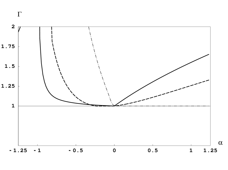
Figure 2: Growth-rate $\Gamma$ with $\Delta t=20\leavevmode\nobreak\ s$ for the EE system with a 2-TL SI scheme as a function of the nonlinearity parameter $\alpha$. solid line: external mode (i); dashed line: slantwise mode (ii); dot-dashed line: internal mode (iii). The left-part of the solid line represents an acoustic external mode.

As a first illustration of the results, the growth-rates of 2-TL non-extrapolating ICI schemes are shown in Fig. 2 as function of $\alpha=(\overline{T}-T^{*})/T^{*}$ with a moderate time-step $\Delta t=20\leavevmode\nobreak\ s$, for three particular mode structures:

(i) an external mode ($k=0.0005\leavevmode\nobreak\ {\rm m}^{-1}$, $\nu=0$)

(ii) a vertical very internal mode ($k=0$, $\nu=100$)

(ii) an intermediate slantwise mode ($k=0.0005\leavevmode\nobreak\ {\rm m}^{-1}$, $\nu=3$)

The suspicions raised in the simple 1D examples are confirmed: the internal vertically-propagating mode is unstable for $\alpha<0$ while the external gravity mode is unstable for $\alpha>0$. Moreover, intermediate, slantwise-propagating modes are unstable in the whole domain, and the acoustic external mode (Lamb-wave) appears to be unstable for $\alpha<0$ as well. The domain of stability vanishes, which confirms that 2-TL SI scheme is not relevant for solving the EE system. The effect of introducing a time-filter to save the situation is discussed below.

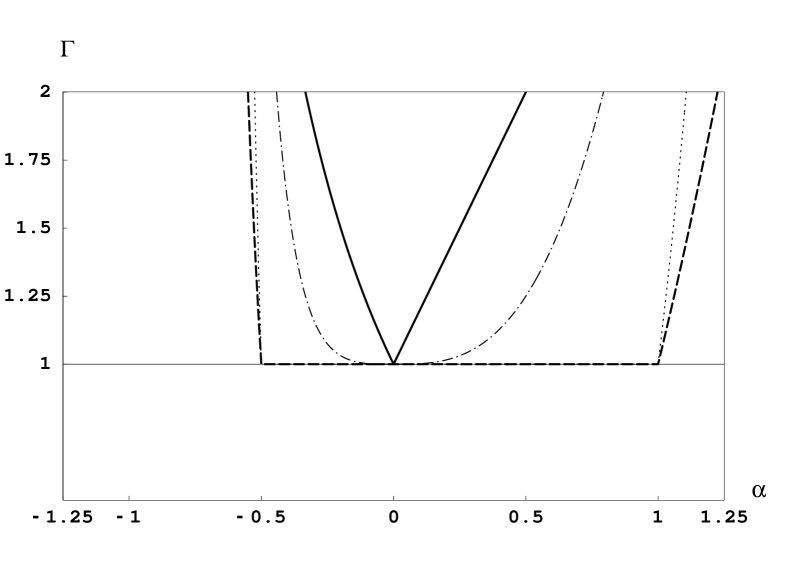
Figure 3: Asymptotic growth-rates $\Gamma$ for EE system with 2-TL ICI scheme as a function of the nonlinearity parameter $\alpha$. solid line: $N_{\rm iter}=1$; dashed line: $N_{\rm iter}=2$; dot-dashed line: $N_{\rm iter}=3$; dotted line: $N_{\rm iter}=4$.

The asymptotic growth-rates resulting from the EE system for $\Delta t=\infty$ are now examined. Similarly to most previous cases, they are independent of the geometry ($k$, $\nu$) of the mode. Fig. 3 shows the asymptotic growth-rates as a function of $\alpha$ for 2-TL non-extrapolating ICI schemes with $N_{\rm iter}=(1,2,3,4)$. As stated above, the SI scheme ($N_{\rm iter}=1$) is unstable for any value of $\alpha$. For even values of $N_{\rm iter}$, the scheme has an "optimal" domain of unconditional stability $-1/2\leq\alpha\leq 1$, while for odd values, the scheme is unstable for all values of $\alpha$.

For 3-TL ICI schemes the domain of unconditional stability is $-1/2\leq\alpha\leq 1$ independently of the values of $N_{\rm iter}$ and $\kappa$. The curves (not shown) are similar to those obtained for even values of $N_{\rm iter}$ for 2-TL ICI schemes.

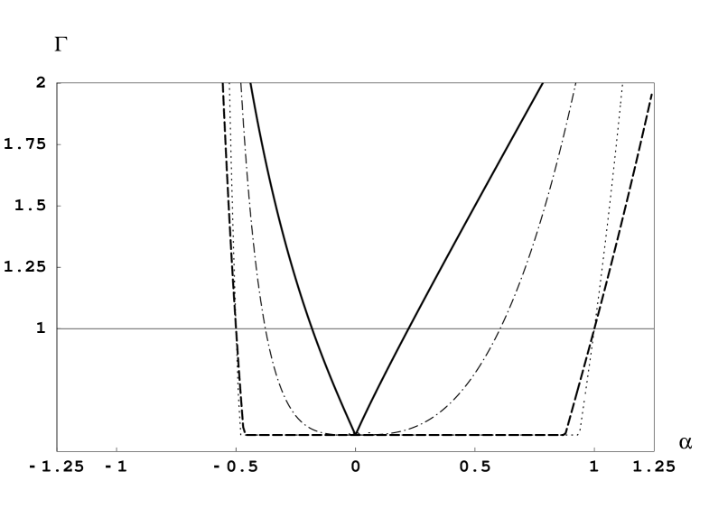
Figure 4: Same as Fig 3, but with a time-filter $\kappa=0.1$. solid line: $N_{\rm iter}=1$; dashed line: $N_{\rm iter}=2$; dot-dashed line: $N_{\rm iter}=3$; dotted line: $N_{\rm iter}=4$.

The impact of applying a time-filter $\kappa=0.1$ to 2-TL ICI schemes is depicted on Fig 4 for the second variant (the first variant behave qualitatively in the same way). The global impact is to "lower" the curves of the asymptotic growth-rates, and consequently, to increase the width of the unconditional-stability domain. However, large values of $\kappa$ (e.g. $\kappa\approx 0.5$) are required in order to obtain a wide stability domain, especially for the 2-TL SI scheme, and this strategy is known to be irrelevant for NWP purpose.

Finally, it is worth noting that the results obtained for the EE system are fully compatible with the conclusions that can be drawn from the intersection of the domains of unconditional stability in Table 1 for the two simple frameworks examined above in mass-coordinate. The ability of these very refined frameworks to capture the essence of the behaviour of the time-discretised EE system in the limit of long time-steps makes them very useful tools to fully understand the underlying causes of its stability or instability.

8 Conclusion

A general method for investigating the stability of the ICI class of time-discretisations on canonical problems with various space-continuous equation systems has been presented. These ICI schemes are based on a separation of evolution terms between a simple linear operator and "non-linear" residuals. The method has been validated by confirming earlier results, then the application to new frameworks (equation systems or time-discretisation schemes) allowed to extend these results. The main conclusions drawn from this study are:

• Even on very simple (1D) examples, the stability properties of time-discretisations for a given equation system are very dependent on fundamental choices (as e.g. the choice of the vertical coordinate). Hence, the import of conclusions drawn from a given analysis must be carefully limited to the examined framework.

• For the EE system, height-based coordinates have a theoretical disavantage compared to mass-based coordinates since they exhibit an intrinsic instability for (long) vertically propagating waves.

• The 2-TL SI scheme is found not to be appropriate for the EE set of equations, whatever coordinate is employed (using a time-filter results in an unacceptable degradation of the solution).

• For the EE system, the 2-TL scheme with $N_{\rm iter}=2$ brings a dramatic increase of the stability compared to the 2-TL SI scheme ($N_{\rm iter}=1$). This statement holds for even values of $N_{\rm iter}$, while odd values leads to a significantly weaker stability.

• As a consequence of the latter point, the 2-TL ICI scheme with $N_{\rm iter}=2$ seems worth to be considered for the EE system.

However, as mentioned in SHB78, the stability inferred from this type of analyses is overestimated, and flows in which the non-linearity comes from other sources than the discrepancy between the atmospheric and reference temperature profiles could reveal new instabilities in practice. For instance, in spite of its apparent "optimal" stability in the simplified context of this paper, the 3-TL SI scheme has proved to be not stable enough for solving numerically the EE system in realistic highly non-linear conditions at high resolutions, due to other terms treated explicitly. This point clearly demonstrates the limitations of this type of academic exercise.

Nevertheless, in spite of its necessary limitations, this study can serve to distinguish schemes which are definitely not relevant for practical use from the others, and give a first theoretical justification for those which are worth considering. In agreement with Cote et al (1998) and Cullen (2000) we think that ICI schemes with $N_{\rm iter}\geq 2$ are among the most approriate alternatives for integrating the EE system in highly non-linear conditions at fine-scale, including from the point of view of efficiency.

References

Bubnová, R., G. Hello, P. Bénard, and J.F. Geleyn, 1995: Integration of the fully elastic equations cast in the hydrostatic pressure terrain-following coordinate in the framework of the ARPEGE/Aladin NWP system. Mon. Wea. Rev., 123, 515-535.

Caya, D., and R. Laprise, 1999: A semi-implicit semi-Lagrangian regional climate model: the Canadian RCM. Mon. Wea. Rev., 127, 341-362.

Côté, J., M. Béland, and A. Staniforth, 1983: Stability of vertical discretization schemes for semi-implicit primitive equation models: theory and application. Mon. Wea. Rev., 111, 1189-1207.

Côté, J., S. Gravel, A. Méthot, A. Patoine, M. Roch, and A. Staniforth, 1998: The Operational CMC-MRB Global Environmental Multiscale (GEM) Model. Part I: Design Considerations and Formulation. Mon. Wea. Rev., 126, 1373-1395.

Cullen, M. J. P., 2000: Alternative implementations of the semi-Lagrangian semi-implicit schemes in the ECMWF model. Q. J. R. Meteorol. Soc., 127, 2787-2802.

Hereil, P., and R. Laprise, 1996: Sensitivity of Internal Gravity Waves Solutions to the Time Step of a Semi-Implicit Semi-Lagrangian Nonhydrostatic Model. Mon. Wea. Rev., 124, 972-999.

Laprise, R., 1992: The Euler equations of motion with hydrostatic pressure as an independent variable. Mon. Wea. Rev., 120, 197-207.

Qian, J.-H., F. H. M. Semazzi, and J. S. Scroggs, 1998: A global nonhydrostatic semi-Lagrangian atmospheric model with orography. Mon. Wea. Rev., 126, 747-771.

Robert, A. J., J. Henderson, and C. Turnbull, 1972: An implicit time integration scheme for baroclinic models of the atmosphere . Mon. Wea. Rev., 100, 329-335.

Semazzi, F. H. M., J. H. Qian, and J. S. Scroggs, 1995: A global nonhydrostatic semi-Lagrangian atmospheric model without orography. Mon. Wea. Rev., 123, 2534-2550.

Simmons, A. J., B. Hoskins, and D. Burridge, 1978: Stability of the semi-implicit method of time integration. Mon. Wea. Rev., 106, 405-412.

Simmons, A. J., C. Temperton, 1997: Stability of a two-time-level semi-implicit integration scheme for gravity wave motion. Mon. Wea. Rev., 125, 600-615.

Tanguay, M., A. Robert, and R. Laprise, 1990: A Semi-Implicit Semi-Larangian Fully Compressible Regional Forecast Model. Mon. Wea. Rev., 118, 1970-1980.

List of Tables

Table 1: Domains of unconditional stability for time-filtered schemes for the two first 1D examples.

	Shallow-water	1D vertical (mass)
3-TL ICI	$-1\leq\alpha\leq 1$	$-1/2\leq\alpha$
2-TL ICI ($N_{\rm iter}$ even)	$-1\leq\alpha\leq 1$	$-1/2\leq\alpha$
2-TL ICI ($N_{\rm iter}$ odd)	$-1\leq\alpha\leq(2\kappa)^{1/N_{\rm iter}}$	$\frac{\textstyle-2\kappa^{(1/N_{\rm iter})}}{\textstyle 1+2\kappa^{(1/N_{\rm iter})}}\leq\alpha$

Table 1: Domains of unconditional stability for time-filtered schemes for the two first 1D examples.

List of Figures

Fig. 1: Asymptotic growth-rates $\Gamma$ for 1D vertical system in $z$ coordinate as a function of the nonlinearity parameter $\alpha$. thin line: long mode ($\nu=0.0001\;{\rm m}^{-1}$) with 2-TL SI scheme; thick line: long mode with 2-TL ICI scheme $N_{\rm iter}=2$; dotted line: external mode ($\nu=0$)with 3-TL SI scheme; dashed line: long mode with 3-TL SI scheme. Circles: practical growth-rate of 3-TL SI scheme for the long mode with $\Delta t=30$ s and $\epsilon=0.1$.

Fig. 2: Growth-rate $\Gamma$ with $\Delta t=20\leavevmode\nobreak\ s$ for the EE system with a 2-TL SI scheme as a function of the nonlinearity parameter $\alpha$. solid line: external mode (i); dashed line: slantwise mode (ii); dot-dashed line: internal mode (iii). The left-part of the solid line represents an acoustic external mode.

Fig. 3: Asymptotic growth-rates $\Gamma$ for EE system with 2-TL ICI scheme as a function of the nonlinearity parameter $\alpha$. solid line: $N_{\rm iter}=1$; dashed line: $N_{\rm iter}=2$; dot-dashed line: $N_{\rm iter}=3$; dotted line: $N_{\rm iter}=4$.

Fig. 4: Same as Fig 3, but with a time-filter $\kappa=0.1$. solid line: $N_{\rm iter}=1$; dashed line: $N_{\rm iter}=2$; dot-dashed line: $N_{\rm iter}=3$; dotted line: $N_{\rm iter}=4$.