Third-order relativistic many-body calculations of energies and lifetimes of levels along the silver isoelectronic sequence

Abstract

Energies of $5l_{j}$ ($l=s,\,p,\,d,\,f,\,g$) and $4f_{j}$ states in neutral Ag and Ag-like ions with nuclear charges $Z=48-100$ are calculated using relativistic many-body perturbation theory. Reduced matrix elements, oscillator strengths, transition rates and lifetimes are calculated for the 17 possible $5l_{j}-5l^{\prime}_{j^{\prime}}$ and $4f_{j}-5l_{j^{\prime}}$ electric-dipole transitions. Third-order corrections to energies and dipole matrix elements are included for neutral Ag and for ions with $Z\leq 60$. Second-order corrections are included for $Z>60$. Comparisons are made with available experimental data for transition energies and lifetimes. Correlation energies and transition rates are shown graphically as functions of nuclear charge $Z$ for selected cases. These calculations provide a theoretical benchmark for comparison with experiment and theory.

I Introduction

This work continues earlier third-order relativistic many-body perturbation theory (RMBPT) studies of energy levels of ions with one valence electron outside a closed core. In Refs. Johnson et al. (1988a, b); Johnson et al. (1990) third-order RMBPT was used to calculate energies of the three lowest states ($ns_{1/2}$, $np_{1/2}$, and $np_{3/2}$) in Li-, Na-, and Cu-like ions along the respective isoelectronic sequences, while in the present work, third-order RMBPT is used to calculate energies of the eleven lowest levels, $5s_{1/2}$, $5p_{j}$, $5d_{j}$, $4f_{j}$, $5f_{j}$, and $5g_{j}$ in Ag-like ions. It should be noted that the $n=1,\,2,\,\text{and }3$ cores of Li-, Na-, and Cu-like ions are completely filled, by contrast with Ag-like ions, where the $n=4$ core [Cu⁺]$4s^{2}4p^{6}4d^{10}$ is incomplete.

Third-order RMBPT calculations of $5s_{1/2}-5p_{j}$ transition amplitudes in Ag-like ions up to $Z$=60 were previously performed by Chou and Johnson (1997). In the present paper, we extend the calculations of Chou and Johnson (1997) to obtain energies, reduced matrix elements, oscillator strengths, and transition rates for the 17 possible $5l_{j}-5l^{\prime}_{j^{\prime}}$ and $4f_{j}-5l_{j^{\prime}}$ E1 transitions. Additionally, we evaluate lifetimes of excited states. Most earlier theoretical studies of Ag-like ions were devoted to oscillator strengths and lifetimes Martin et al. (1995); Migdalek and Baylis (1979) rather than energy levels; an exception is the work of Cheng and Kim (1979) in which energies, oscillator strengths and lifetimes of levels in Ag-like ions were calculated using relativistic Dirac-Fock (DF) wave functions Desclaux (1975). In the present paper, we use RMBPT to determine energies and lifetimes of $4f_{j}$ and $5l_{j}$ levels in neutral Ag and Ag-like ions with $Z=48-100$. We compare our results with experimental data from Refs. Carlsson et al. (1990); Andersen et al. (1976); Pinnington et al. (1994); Ansbacher et al. (1986); Pinnington et al. (1987); Pinnington et al. (1985a, b); Ansbacher et al. (1991); Sugar (1977).

Table 1: Contributions to energy levels of Ag-like ions in cm^-1.

$nlj$	$E^{(0)}$	$E^{(2)}$	$E^{(3)}$	$B^{(1)}$	$B^{(2)}$	$E_{\rm LS}$	$E_{\rm tot}$		$E^{(0)}$	$E^{(2)}$	$E^{(3)}$	$B^{(1)}$	$B^{(2)}$	$E_{\rm LS}$	$E_{\rm tot}$
$Z$=47									$Z$=48
$5s_{1/2}$	-50376	-11173	3139	83	-180	138	-58369		-124568	-13505	3321	150	-264	162	-134703
$5p_{1/2}$	-26730	-4217	680	34	-60	-2	-30296		-84903	-7731	1614	107	-143	-3	-91058
$5p_{3/2}$	-26148	-3872	617	23	-50	7	-29423		-82871	-7176	1477	76	-130	8	-88615
$5d_{3/2}$	-11982	-328	36	1	-11	-2	-12287		-45147	-1531	236	14	-36	-2	-46466
$5d_{5/2}$	-11967	-323	34	1	-12	2	-12265		-45010	-1503	230	11	-38	2	-46308
$4f_{5/2}$	-6860	-37	5	0	0	-2	-6894		-27540	-361	53	0	0	-2	-27850
$4f_{7/2}$	-6860	-37	5	0	0	2	-6890		-27543	-361	52	0	0	2	-27849
$5f_{5/2}$	-4391	-33	10	0	0	-1	-4414		-17644	-221	30	0	0	-1	-17836
$5f_{7/2}$	-4391	-33	10	0	0	1	-4412		-17646	-221	30	0	0	1	-17837
$5g_{7/2}$	-4389	-6	3	0	0	-1	-4394		-17559	-49	7	0	0	-1	-17601
$5g_{9/2}$	-4389	-6	3	0	0	1	-4392		-17559	-49	7	0	0	1	-17599
$Z$=53									$Z$=54
$5s_{1/2}$	-692263	-18545	4916	586	-564	327	-705543		-839765	-19240	5054	698	-628	371	-853511
$5p_{1/2}$	-589599	-15210	3861	673	-442	-4	-600720		-725343	-16192	4100	825	-508	-4	-737122
$5p_{3/2}$	-575199	-14239	3611	483	-417	20	-585742		-707377	-15159	3839	592	-480	23	-718562
$4f_{5/2}$	-419424	-16897	3699	197	-790	-5	-433221		-572051	-20265	4554	306	-1108	-6	-588570
$4f_{7/2}$	-419399	-16631	3629	131	-773	5	-433037		-571685	-19938	4469	205	-1085	5	-588028
$5d_{3/2}$	-425432	-8511	1929	229	-272	0	-432058		-536495	-9746	2228	298	-334	0	-544048
$5d_{5/2}$	-423242	-8370	1895	178	-277	5	-429812		-533632	-9578	2186	232	-340	6	-541127
$5f_{5/2}$	-264311	-6586	1591	82	-305	-2	-269531		-350670	-7548	1821	105	-345	-2	-356640
$5f_{7/2}$	-264076	-6513	1529	55	-301	2	-269303		-350271	-7488	1804	72	-342	2	-356224
$5g_{7/2}$	-215806	-1723	319	1	-4	-2	-217214		-282283	-2442	457	2	-7	-2	-284276
$5g_{9/2}$	-215811	-1722	319	0	-4	2	-217215		-282292	-2440	456	0	-7	2	-284280
$Z$=57								$Z$=58
$5s_{1/2}$	-1345535	-21098	5350	1092	-832	526	-1360497		-1534879	-21658	5423	1243	-903	586	-1550187
$4f_{5/2}$	-1149152	-26307	5919	695	-1956	-8	-1170808		-1376678	-27562	6137	844	-2217	-9	-1399486
$4f_{7/2}$	-1147163	-25901	5820	474	-1921	8	-1168685		-1373977	-27142	6036	577	-2180	9	-1396676
$5p_{1/2}$	-1196202	-18769	4647	1367	-717	-4	-1209677		-1373944	-19536	4790	1578	-791	-4	-1387907
$5p_{3/2}$	-1164895	-17563	4363	980	-678	36	-1177757		-1337210	-18278	4500	1129	-747	41	-1350564
$5d_{3/2}$	-932064	-13156	3000	558	-536	0	-942198		-1084072	-14211	3221	663	-608	0	-1095007
$5d_{5/2}$	-926588	-12895	2929	433	-543	9	-936655		-1077506	-13912	3139	514	-617	10	-1088372
$5f_{5/2}$	-669070	-11088	2495	192	-475	-4	-677951		-794882	-12370	2713	230	-529	-5	-804843
$5f_{7/2}$	-668137	-11029	2479	134	-475	4	-677023		-793733	-12300	2694	162	-529	5	-803702
$5g_{7/2}$	-536613	-5673	1042	0	-27	-4	-541275		-639897	-7286	1284	9	-39	-5	-645935
$5g_{9/2}$	-536641	-5647	1039	0	-27	4	-541271		-639931	-7232	1282	4	-38	5	-645910

Table 2: Contributions to the correlation energies of $4f$ and $5l$ states of Pm¹⁴⁺ in cm^-1.

	$E^{(2)}_{l\leq 6}$	$E^{(2)}$	$E^{(2)}_{l>6}$	$E^{(3)}_{l\leq 6}$	$E^{(3)}_{l>6}$
$5s_{1/2}$	-22892	-23111	-218	5593	53
$4f_{5/2}$	-28621	-30123	-1501	6454	338
$4f_{7/2}$	-28170	-29661	-1491	6352	336
$5p_{1/2}$	-21377	-21632	-255	5139	61
$5p_{3/2}$	-19996	-20232	-235	4837	57
$5d_{3/2}$	-16956	-17178	-222	3800	50
$5d_{5/2}$	-16534	-16752	-218	3677	48
$5f_{5/2}$	-15891	-16179	-288	3296	60
$5f_{7/2}$	-15763	-16050	-287	3265	59
$5g_{7/2}$	-17572	-17880	-308	434	8
$5g_{9/2}$	-16846	-17152	-306	788	14

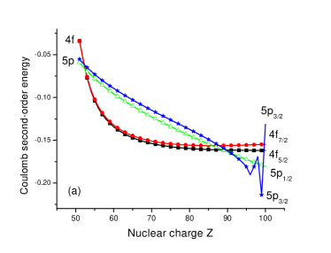
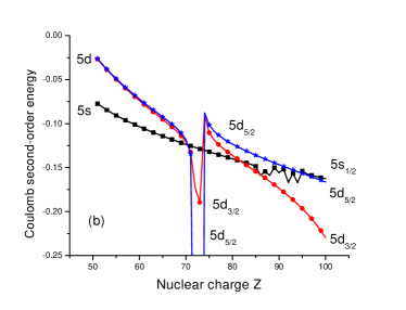
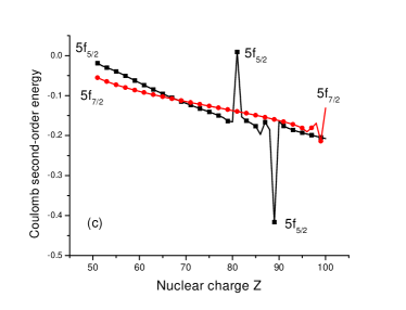
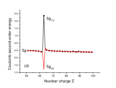
Figure 1: Coulomb second-order contributions to valence energies in Ag-like ions in atomic units.

II Energy levels of Ag-like ions

Results of our third-order calculations of energies, which were carried out following the pattern described in Johnson et al. (1988a), are summarized in Table 1, where we list lowest-order, Dirac-Fock energies $E^{(0)}$, first-order Breit energies $B^{(1)}$, second-order Coulomb $E^{(2)}$ and Breit $B^{(2)}$ energies, third-order Coulomb energies $E^{(3)}$, single-particle Lamb shift corrections $E_{\rm LS}$, and the sum of the above $E_{\text{tot}}$. The first-order Breit energies $B^{(1)}$ include corrections for “frequency-dependence”, whereas second-order Breit energies are evaluated using the static Breit operator. The Lamb shift $E_{\text{LS}}$ is approximated as the sum of the one-electron self energy and the first-order vacuum-polarization energy. The vacuum-polarization contribution is calculated from the Uehling potential using the results of Fullerton and Rinker Fullerton and G. A. Rinker, Jr. (1976). The self-energy contribution is estimated for $s$, $p_{1/2}$ and $p_{3/2}$ orbitals by interpolating among the values obtained by Mohr (1974a, b, 1975) using Coulomb wave functions. For this purpose, an effective nuclear charge $Z_{\rm eff}$ is obtained by finding the value of $Z_{\rm eff}$ required to give a Coulomb orbital with the same average $\langle r\rangle$ as the DHF orbital.

We find that correlation corrections to energies in neutral Ag and in low-$Z$ Ag-like ions are large, especially for $5s$ states. For example, $E^{(2)}$ is 22% of $E^{(0)}$ and $E^{(3)}$ is 28% of $E^{(2)}$ for the $5s$ state of neutral Ag. These ratios decrease for the other (less penetrating) states and for more highly charged ions. Despite the slow convergence of the perturbation expansion, the $5s$ energy from the present third-order RMBPT calculation is within 5% of the measured ionization energy for the $5s$ state of neutral Ag and improves for higher valence states and for more highly charged ions. We include results for neutral Ag and five Ag-like ions with $Z$ = 48, 53, 54, 57, and 58 in Table 1. For each ion, the states are ordered by energy and the order changes with $Z$. For example, the $4f_{5/2}$ and $4f_{7/2}$ states are in the sixth and seventh places for neutral Ag and Ag-like ions with the nuclear charge $Z<53$, in the fourth and fifth places for ions with $Z=53-56$, the second and third places for ions with $Z=57-60$, and the first and second places for ions with $Z\geq 62$. It should be mentioned that the difference in energies of $5s$ and $4f_{5/2}$ states is about 244 cm^-1 for $Z$ = 61 which may exceed the accuracy of the present calculations.

Below, we describe a few numerical details of the calculation for a specific case, Pm¹⁴⁺ ($Z=61$). We use B-spline methods Johnson et al. (1988c) to generate a complete set of basis DF wave functions for use in the evaluation of RMBPT expressions. For Pm¹⁴⁺, we use 40 splines of order $k=7$ for each angular momentum. The basis orbitals are constrained to a cavity of radius 10 $a_{0}$ for Pm¹⁴⁺, where $a_{0}\approx 0.052918$ nm is Bohr radius. The cavity radius is scaled for different ions; it is large enough to accommodate all $5l_{j}$ and $4f_{j}$ orbitals considered here and small enough that 40 splines can approximate inner-shell DF wave functions with good precision. We use 35 out 40 basis orbitals for each partial wave in our third-order energy calculations, since contribution of the five highest-energy orbitals is negligible. The second-order calculation includes partial waves up to $l_{\text{max}}=8$ and is extrapolated to account for contributions from higher partial waves. A lower number of partial waves, $l_{\text{max}}=6$, is used in the third-order calculation. We list the second-order energy with $l_{\text{max}}=6$, the final value of $E^{(2)}$ extrapolated from $l_{\text{max}}=8$ and the contribution from partial waves with $l>6$ in Table 2. Since the asymptotic $l$-dependence of the second- and third-order energies are similar (both fall off as $l^{-4}$), we may use the second-order remainder as a guide to extrapolating the third-order energy, which is listed, together with an estimated remainder from $l>6$ in the fifth and sixth columns of Table 2. We find that the contribution to the third-order energy from states with $l>6$ is more than 300 cm^-1 for $4f$ states of Pm¹⁴⁺.

Table 3: Comparison of the energies of the $4f$ and $5l$ states in Ag-like ions with experimental data Moore (1971). Units: cm^-1.

$nlj$	$E_{\text{tot}}$	$E_{\text{expt}}$	$\delta E$	$E_{\text{tot}}$	$E_{\text{expt}}$	$\delta E$	$E_{\text{tot}}$	$E_{\text{expt}}$	$\delta E$	$E_{\text{tot}}$	$E_{\text{expt}}$	$\delta E$
	$Z$=47			$Z$=48			$Z$=49			$Z$=50
$5s_{1/2}$	-58369	-61106	2737	-134703	-136375	1672	-224666	-226100	1434	-327453	-328550	1097
$5p_{1/2}$	-30296	-31554	1258	-91058	-92239	1181	-167850	-168919	1069	-258188	-258986	798
$5p_{3/2}$	-29423	-30634	1211	-88615	-89756	1141	-163546	-164577	1031	-251717	-252478	761
$5d_{3/2}$	-12287	-12362	75	-46466	-46686	220	-97584	-97647	63	-162915	-163245	330
$5d_{5/2}$	-12265	-12342	77	-46308	-46532	224	-97176	-97358	182	-162170	-163139	969
$4f_{5/2}$	-6894	-6901	7	-27850	-27956	106	-63903	-64131	228	-117959	-118232	273
$4f_{7/2}$	-6890	-6901	11	-27849	-27943	94	-63922	-64123	201	-118035	-118292	257
$5f_{5/2}$	-4414	-4415	1	-17836	-17931	95	-41032			-76428
$5f_{7/2}$	-4412	-4415	3	-17837	-17829	-8	-41049			-76472
$5g_{7/2}$	-4394	-4395	1	-17601	-17605	4	-39656	-39578	-78	-70585	-70267	-318
$5g_{9/2}$	-4392	-4395	3	-17599	-17605	6	-39654	-39578	-76	-70581	-70268	-313

In Fig. 1, we illustrate the $Z$ dependence of the second-order energy $E^{(2)}$ given in atomic units for $4f$, $5s$, $5p$, $5d$, $5f$, and $5g$ states of Ag-like ions. The atomic unit (a.u.) of energy is $E_{h}\approx 4.3597\times 10^{-18}$ J, where $E_{h}$ is Hartree energy.

As we see from this figure $|E^{(2)}|$ slowly increases with $Z$ for most values of $Z$. We observe several sharp features in the curves describing $5d_{3/2}$ states ($Z=72$), $5f_{5/2}$ states ($Z=89$), and $5g_{7/2}$ states ($Z=63$). These irregularities have their origin in the near degeneracy of one-electron valence states with two-particle one-hole states of the same angular symmetry, resulting in exceptionally small energy denominators in double-excitation contributions to the second-order energy. To remove these irregularities, the perturbative treatment should be based on a lowest-order wave function that includes both one-particle and two-particle one-hole states. The singularities in the second-order $5d_{3/2}$ energy at $Z=72$ in Fig. 1, for example, occurs because the lowest-order $5d_{3/2}$ energy, $\epsilon_{5d_{3/2}}=-19.2215$ a.u. is nearly degenerate with the lowest-order energy of the $(4d_{5/2})^{-1}(4f_{5/2})^{2}$ state: $-\epsilon_{4d_{5/2}}+2\epsilon_{4f_{5/2}}=36.8850-2\times 28.0685=-19.2520$ a.u.. The other singularities seen in Fig. 1 have similar explanations.

Results and comparisons for energies

As discussed above, starting from $Z=62$ the second-order energy for one-particle states has irregularities associated with nearly degenerate two-particle one-hole states. These near degeneracies, of course, lead to similar irregularities in the third-order valence energy. The importance of third-order corrections decreases substantially with $Z$, it contributes 6% to the total energy of the $5s$ state for neutral Ag but only 0.3% to the total energy of the $5s$ state of Ag-like Ce, $Z=58$. Thus, omission of the third-order corrections is justified for ions with $Z>60$.

Table 4: Dipole oscillator strengths ($f$) for transitions in Ag-like ions.

	$5s$-$5p_{j^{\prime}}$			$5p_{j}$-$5d_{j^{\prime}}$				$4f_{j}$-$5d_{j^{\prime}}$				$4f_{j}$-$5g_{j^{\prime}}$
$Z$	1/2-1/2	1/2-3/2		1/2-3/2	3/2-3/2	3/2-5/2		5/2-3/2	5/2-5/2	7/2-5/2		5/2-7/2	7/2-7/2	7/2-9/2
47	0.2497	0.5134		0.5773	0.0613	0.5491		1.0118	0.0484	0.9678		1.3800	0.0383	1.3405
48	0.2548	0.5423		0.8097	0.0841	0.7540		1.1007	0.0527	1.0536		1.2814	0.0356	1.2452
49	0.2519	0.5478		0.9113	0.0932	0.8387		1.0915	0.0520	1.0394		1.2084	0.0335	1.1736
50	0.2489	0.5508		0.9577	0.0968	0.8736		0.8751	0.0413	0.8251		1.0093	0.0280	0.9797
51	0.2456	0.5521		0.9781	0.0978	0.8856		0.4851	0.0226	0.4503		0.7564	0.0210	0.7357
52	0.2419	0.5522		0.9846	0.0975	0.8854		0.1580	0.0071	0.1419		0.5454	0.0152	0.5331
53	0.2380	0.5515		0.9833	0.0965	0.8785		0.0073	0.0009	0.0126		0.4256	0.0119	0.4180
54	0.2340	0.5503		0.9773	0.0950	0.8677		0.0582	0.0044	0.0654		0.3646	0.0102	0.3595
55	0.2299	0.5490		0.9684	0.0933	0.8546		0.0804	0.0058	0.0882		0.3325	0.0093	0.3287
56	0.2259	0.5475		0.9580	0.0915	0.8403		0.0899	0.0065	0.0978		0.3123	0.0088	0.3097
57	0.2219	0.5461		0.9467	0.0896	0.8254		0.0936	0.0067	0.1013		0.2939	0.0083	0.2927
58	0.2179	0.5448		0.9350	0.0877	0.8103		0.0944	0.0067	0.1019		0.2681	0.0075	0.2693
59	0.2141	0.5435		0.9232	0.0858	0.7955		0.0939	0.0066	0.1011		0.2221	0.0061	0.2287
60	0.2103	0.5428		0.9118	0.0840	0.7805		0.0928	0.0065	0.0997		0.1257	0.0025	0.1514

We compare our results for energy levels of the $5l_{j}$ and $4f_{j}$ states with recommended data from the National Institute of Standards and Technology (NIST) database Moore (1971) in neutral Ag and Ag-like ions with $Z=48-50$ in Table 3. Although our results are generally in good agreement with the NIST data, discrepancies were found. One cause for the discrepancies is that fourth- and higher-order correlation corrections are omitted in the theory. Another possible cause may be the large uncertainties in the experimental ionization potentials of ions with $Z=49$ and 50 in Ref. Moore (1971). We also find unusually large discrepancies in the values of $5d_{3/2}-5d_{5/2}$ splittings for ions with $Z=49$ and 50. Additional tables are included in the accompanying EPAPS document Ref. EPA , where we give energies of $5l_{j}$ and $4f_{j}$ states in Ag-like ions for the entire isoelectronic sequence up to $Z=100$.

III Line strengths, oscillator strengths, transition rates, and lifetimes in Ag-like ions

We calculate reduced electric-dipole matrix elements using the gauge-independent third-order perturbation theory developed in Savukov and Johnson (2000). The precision of this method has been demonstrated for alkali-metal atoms. Gauge-dependent “bare” dipole matrix elements are replaced with gauge-independent random-phase approximation (RPA) matrix elements to obtain gauge-independent third-order matrix elements. As in the case of the third-order energy, a limited number of partial waves with $l_{\text{max}}<7$ is included. This restriction is not very important for the ions considered here because the third-order correction is quite small, but the truncation gives rise to some loss of gauge invariance.

Table 5: Line strengths (a.u.) for E1 transitions in Ag-like xenon ($Z$ = 54) calculated in lowest order (DF approximation) $S^{(1)}$, second order $S^{(2)}$, and third order $S^{(3)}$. The first-order result, which is gauge-dependent, is given in length form. The second-, and third-order results are gauge independent.

Transition	$S^{(1)}$	$S^{(2)}$	$S^{(3)}$
$5s_{1/2}-5p_{1/2}$	1.876	1.263	1.324
$5s_{1/2}-5p_{3/2}$	3.774	2.564	2.685
$5p_{1/2}-5d_{3/2}$	4.399	3.279	3.333
$5p_{3/2}-5d_{3/2}$	0.939	0.707	0.717
$5p_{3/2}-5d_{5/2}$	8.416	6.350	6.439
$4f_{5/2}-5d_{3/2}$	3.251	2.734	2.583
$4f_{5/2}-5d_{5/2}$	0.229	0.194	0.182
$4f_{7/2}-5d_{5/2}$	4.618	3.904	3.671
$4f_{5/2}-5g_{7/2}$	3.250	2.680	2.367
$4f_{7/2}-5g_{7/2}$	0.121	0.100	0.089
$4f_{7/2}-5g_{9/2}$	4.254	3.514	3.117

We solve the core RPA equations iteratively. In our calculations, we set the number of core iteration to 10 to save computation time; for convergence to machine accuracy, about 50 iterations are needed at low $Z$. For example, for the $5p_{3/2}-5s$ transition in neutral Ag, first-order length and velocity matrix elements are 4.30225 and 4.26308, respectively. The values of the electric-dipole matrix elements are given in atomic units, $ea_{0}$. The atomic unit for the corresponding line strength is $e^{2}a_{0}^{2}$. The corresponding RPA values are 3.77755 and 3.96707 after one iteration; they become 3.82599 and 3.82636 after 10 iterations. The final third-order gauge-independent results are 3.41726 and 3.41745 for this matrix element in length and velocity forms, respectively.

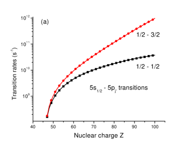
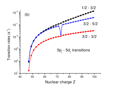
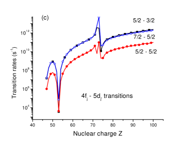
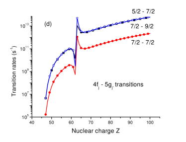
Figure 2: Transition rates (s^-1) in Ag-like ions.

Table 6: Lifetimes ${\tau}$ in ns of the $5l$ and $4f$ levels in Cd¹⁺, In²⁺, Sn³⁺, Sb⁴⁺, Te⁵⁺, I⁶⁺, and Xe⁷⁺. The lifetime of the upper level is shown. The corresponding wavelengths $\lambda$ in Å  are also given. In the cases where more then one transition is allowed the wavelength of the dominant transition is given. The data are compared with experimental results.

Lower	Upper	$\tau^{(1)}$	$\tau^{(2)}$	$\tau^{(3)}$	$\tau^{\text{expt}}$	$\lambda^{(3)}$	$\lambda^{\text{expt}}$
Ag I, $Z$=47
$5s_{1/2}$	$5p_{3/2}$	7.50	5.71	6.97	6.72$\pm$0.03	3455	3282
$5s_{1/2}$	$5p_{1/2}$	7.98	6.24	7.62	7.41$\pm$0.04	3562	3384
Ag-like Cd, $Z$=48
$5d_{5/2}$	$4f_{7/2}$	5.82	5.12	5.57	6.7 $\pm$0.2	5417	5380
$5d_{3/2}$	$4f_{5/2}$	6.16	5.41	5.90	6.2 $\pm$0.1	5372	5338
$5s_{1/2}$	$5p_{3/2}$	2.32	2.42	2.60	2.77$\pm$0.07	2170	2145
$5s_{1/2}$	$5p_{1/2}$	2.68	2.88	3.09	3.11$\pm$0.04	2291	2266
$5p_{3/2}$	$5d_{5/2}$	1.75	1.44	1.67	1.85$\pm$0.15	2364	2314
$5p_{1/2}$	$5d_{3/2}$	1.95	1.60	1.86	1.79$\pm$0.11	2243	2195
Ag-like In, $Z$=49
$4f_{7/2}$	$5g_{9/2}$	2.79	2.52	2.71	2.84$\pm$0.30	4121	4072
$5d_{5/2}$	$4f_{7/2}$	1.71	1.62	1.74	1.72$\pm$0.07	3007	3009
$5d_{3/2}$	$4f_{5/2}$	1.78	1.69	1.82	1.70$\pm$0.07	2969	2983
$5s_{1/2}$	$5p_{3/2}$	1.20	1.42	1.45	1.50$\pm$0.15	1630	1625
$5s_{1/2}$	$5p_{1/2}$	1.48	1.81	1.84	1.64$\pm$0.06	1760	1749
$5p_{3/2}$	$5d_{5/2}$	0.58	0.56	0.61	0.58$\pm$0.05	1507	1488
$5p_{1/2}$	$5d_{3/2}$	0.64	0.61	0.67	0.75$\pm$0.06	1423	1403
Ag-like Sn, $Z$=50
$5d_{5/2}$	$4f_{7/2}$	1.20	1.27	1.38	1.30$\pm$0.20	2266	2230
$5d_{3/2}$	$4f_{5/2}$	0.98	1.04	1.13	1.25$\pm$0.20	2224	2222
$5s_{1/2}$	$5p_{3/2}$	0.75	0.95	0.95	0.81$\pm$0.15	1320	1315
$5s_{1/2}$	$5p_{1/2}$	0.97	1.27	1.26	1.29$\pm$0.20	1444	1438
$5p_{3/2}$	$5d_{5/2}$	0.29	0.31	0.32	0.45$\pm$0.05	1117	1119
$5p_{1/2}$	$5d_{3/2}$	0.31	0.33	0.34	0.34$\pm$0.04	1050	1044
Ag-like Sb, $Z$=51
$5d_{5/2}$	$4f_{7/2}$	1.77	2.23	2.57	2.5$\pm$0.4	2268	2279
$5d_{3/2}$	$4f_{5/2}$	1.38	1.73	2.00	2.4$\pm$0.3	2202	2217
$5s_{1/2}$	$5p_{3/2}$	0.51	0.68	0.67	0.65$\pm$0.12	1108	1104
$5s_{1/2}$	$5p_{1/2}$	0.70	0.95	0.92	0.77$\pm$0.10	1230	1226
$5p_{3/2}$	$5d_{5/2}$	0.18	0.20	0.20		892.1
$5p_{1/2}$	$5d_{3/2}$	0.18	0.21	0.21	0.191$\pm$0.020	834.1	831
Ag-like Te, $Z$=52
$5s_{1/2}$	$5p_{3/2}$	0.38	0.510	0.493	0.47$\pm$0.03	952.9	951
$5s_{1/2}$	$5p_{1/2}$	0.58	0.738	0.713	0.65$\pm$0.04	1073	1071
$5p_{3/2}$	$5d_{5/2}$	0.12	0.140	0.141	0.13$\pm$0.03	745.3	743
$5p_{1/2}$	$5d_{3/2}$	0.12	0.146	0.146	0.14$\pm$0.04	693.0	691
Ag-like I, $Z$=53
$5s_{1/2}$	$5p_{3/2}$	0.29	0.39	0.38	0.35$\pm$0.02	834.7
$5s_{1/2}$	$5p_{1/2}$	0.43	0.60	0.57	0.48$\pm$0.03	954.0
$5p_{3/2}$	$5d_{5/2}$	0.087	0.106	0.105	0.107$\pm$0.016	641.3	640
$5p_{1/2}$	$5d_{3/2}$	0.090	0.108	0.107	0.120$\pm$0.020	592.9	592
Ag-like Xe, $Z$=54
$5s_{1/2}$	$5p_{3/2}$	0.23	0.31	0.30	0.33$\pm$0.03	741.0	740.4
$5s_{1/2}$	$5p_{1/2}$	0.35	0.50	0.47	0.50$\pm$0.05	858.6	859.2

The results of our third-order calculations are summarized in Table 4, where we list oscillator strengths for $5s-5p$, $5p-5d$, $4f-5d$, and $4f-5g$ transitions in neutral Ag and low-$Z$ Ag-like ions with $Z=48-60$.

In Table 5, we present line strengths for $5s-5p$, $5p-5d$, $4f-5d$, and $4f-5g$ transitions in Xe⁷⁺. The values calculated in length form in first, second, and third approximations are listed in columns $S^{(1)}$, $S^{(2)}$, and $S^{(3)}$, respectively. The difference between second-order values $S^{(2)}$ and third-order values $S^{(3)}$ is much smaller than the difference between $S^{(1)}$ and $S^{(2)}$. The second-order corrections change $S^{(1)}$ by 20 - 50 %. The addition of the third-order corrections modifies line strengths by 5 - 10 %. The first approximation is just the frozen-core DF approximation and the first-order line strengths $S^{(1)}$ in Table 5 are very close to the earlier DF calculations by Cheng and Kim (1979).

$Z$ dependence of transition rates

Trends of the $Z$ dependence of transition rates are shown in Fig. 2. The $5s-5p$, $5p-5d$, $4f-5d$, and $4f-5g$ transition rates are shown in Fig. 2 a, b, c, d, respectively. All graphs are plotted using second-order data for consistency. The $Z$ dependences of the transition rates for $5s-5p$ transitions shown in Fig. 2a and two $5p-5d$ transitions shown in Fig. 2b are smooth; however, all other $Z$ dependences shown in Fig. 2 contain sharp features. The sharp feature in the curve describing the $5p_{3/2}-5d_{5/2}$ transition rates (Fig. 2b) is explained by irregularity in the curve describing the $5d_{5/2}$ energy shown in Fig. 1b. This irregularity in the energy $Z$ dependence was already discussed in the previous section.

The sharp minima in the region $Z=52-54$ in the curves describing the $4f-5d$ transition rates shown in Fig. 2c are due to inversion of the order of $4f$ and $5d$ energy levels. In the region $Z=52-54$ the $4f-5d$ transition energies become very small resulting in the small transition rates. The second sharp feature in the curves describing the $4f-5d$ transition rates shown in Fig. 2c occurs in the region $Z$ = 72 - 73 and results from the irregularity in the second-order correction to the $4f-5d$ dipole matrix elements. Below, we describe some details of the calculation to clarify this issue.

A typical contribution from one of the second-order RPA corrections to dipole matrix element ($v-v^{\prime}$) has the form Safronova et al. (1999)

$$D^{{(\rm RPA)}}[v-v^{\prime}]\propto\sum_{nb}\sum_{k}\frac{D_{nb}X_{k}(vnv^{\prime}b)}{\epsilon_{n}+\epsilon_{v}-\epsilon_{v^{\prime}}-\epsilon_{b}}\,.$$ (1)

Here, the index $b$ designates a core state and index $n$ designates an excited state. The numerator is a product of a dipole matrix element $D_{nb}$ and a Coulomb matrix element $X_{k}(vnv^{\prime}b)$. For the special case of the $4f_{5/2}-5d_{3/2}$ transition, the energy denominator for the term in the sum with $n=4f_{5/3}$ and $b=4d_{5/2}$ is

$$\epsilon_{n}+\epsilon_{v}-\epsilon_{v^{\prime}}-\epsilon_{b}$$ (2)

$$=\epsilon_{4f_{5/2}}+\epsilon_{4f_{5/2}}-\epsilon_{5d_{3/2}}-\epsilon_{4d_{5/2}}$$

$$=-28.0685-28.0685+19.2215+36.8850$$

$$=-0.0305.$$

Again, as in the case of the second-order $4d_{3/2}$ energy, there is a nearly zero denominator when the lowest-order energies of the $5d_{3/2}$ and $(4d_{5/2})^{-1}(4f_{5/2})^{2}$ states are close. The cause of this irregularity is once again traced to the near degeneracy of a single-particle state and a two-particle one-hole state. The remaining irregularities for $Z>60$ in the curves presented in Fig. 2 have similar origins.

Results and comparison for lifetimes

We calculate lifetimes of $5l_{j}$ and $4f_{j}$ levels in neutral Ag and in Ag-like ions with $Z=48-60$ using third-order MBPT results for dipole matrix elements and energies. In Table 6, we compare our lifetime data with available experimental measurements. This set of data includes results for a limited number of levels in low-$Z$ ions (up to $Z=54$). We give a more complete comparison of the transition rates and wavelengths for the eleven transitions between $5l$ and $4f$ states in Ag-like ions with $Z=47-60$ including the third-order contribution in Table III of the accompanying EPAPS document EPA . In Table 6, we present our lifetime data $\tau$ calculated in the lowest-, second-, and third-order approximations. These results are listed in columns labeled $\tau^{(1)}$, $\tau^{(2)}$, and $\tau^{(3)}$, respectively. The largest difference between the calculations in different approximations occurs for $5d_{3/2}$ and $5d_{5/2}$ levels for $Z$ = 51 and 52 when $5d-4f$ transition energies become very small and contributions from the second and third orders become very important. It should be noted that for some levels of neutral Ag and Ag-like ions with $Z$ = 48 and 49, $\tau^{(3)}$ agrees better with $\tau^{(1)}$ than with $\tau^{(2)}$. The accuracy of lifetime measurements is not very high for Ag-like ions, and in some cases the lowest-order results $\tau^{(1)}$, which are equivalent to the Dirac-Fock results of Cheng and Kim (1979) were enough to predict the lifetimes. The more sophisticated theoretical studies published recently in Refs. Chou and Johnson (1997); Martin et al. (1995) were restricted to $5s-5p$ transitions and did not include wavelength data. In two last columns of Table 6, we compare our theoretical wavelengths, $\lambda^{(3)}$ with experimental measurements, $\lambda^{\text{expt}}$. In the cases where more than one transition is allowed, the wavelength of the dominant transition is given. We find good agreement, 0.01 - 1%, of our wavelength results with available experimental data for ions with $Z>49$.

IV Conclusion

In summary, a systematic RMBPT study of the energies of $5s_{1/2}$, $5p_{1/2}$, $5p_{3/2}$, $5d_{3/2}$, $5d_{5/2}$, $4f_{5/2}$, $4f_{7/2}$, $5f_{5/2}$, $5f_{7/2}$, $5g_{7/2}$, and $5g_{9/2}$ states in Ag-like ions is presented. These energy calculations are found to be in good agreement with existing experimental energy data and provide a theoretical reference database for the line identification. A systematic relativistic RMBPT study of reduced matrix elements, line strengths, oscillator strengths, and transition rates for the 17 possible $5s-5p$, $5p-5d$, $4f-5d$, and $4f-5g$ electric-dipole transitions in Ag-like ions throughout the isoelectronic sequence up to $Z=100$ is conducted. Both length and velocity forms of matrix elements are evaluated. Small differences between length and velocity-form calculations, caused by the nonlocality of the DF potential, are found in second order. However, including third-order corrections with full RPA leads to complete agreement between the length- and velocity-form results.

We believe that our energies and transition rates will be useful in analyzing existing experimental data and planning new experiments. There remains a paucity of experimental data for many of the higher ionized members of this sequence, both for term energies and for transition probabilities and lifetimes.