Forced Stratified Turbulence:
Successive Transitions with Reynolds Number

Abstract

Numerical simulations are made for forced turbulence at a sequence of increasing values of Reynolds number, $R$, keeping fixed a strongly stable, volume-mean density stratification. At smaller values of $R$, the turbulent velocity is mainly horizontal, and the momentum balance is approximately cyclostrophic and hydrostatic. This is a regime dominated by so-called pancake vortices, with only a weak excitation of internal gravity waves and large values of the local Richardson number, $Ri$, everywhere. At higher values of $R$ there are successive transitions to (a) overturning motions with local reversals in the density stratification and small or negative values of $Ri$; (b) growth of a horizontally uniform vertical shear flow component; and (c) growth of a large-scale vertical flow component. Throughout these transitions, pancake vortices continue to dominate the large-scale part of the turbulence, and the gravity wave component remains weak except at small scales.

I Introduction

Most atmospheric and oceanic flows on intermediate scales of ${\cal O}(1)-{\cal O}(10^{3})$ m are strongly influenced by the stable vertical density stratification, $d\overline{\rho}(z)/dz<0$ (with $\hat{\bf z}={\bf e}_{3}$ anti-parallel to gravity), but are less influenced by Earth’s rotation than flows on larger scales. Consequently, the turbulence in this regime is quite different from unstratified shear turbulence, convection, and geostrophic turbulence, all of which have been more extensively studied and whose behaviors are now relatively familiar. It has been argued lilly83 that the main effect of strongly stable stratification — i.e., small Froude number, $Fr=V/NL_{v}$, where $V$ is a horizontal velocity scale, $N=-(g/\rho_{o})\,d\overline{\rho}/dz$ is the Brünt Väïssäla frequency, and $L_{v}$ is vertical length scale — is to organize the flow into two distinct, non-interacting classes: nearly linear internal gravity waves and fully nonlinear stratified turbulence. The flow patterns of stratified turbulence are often called pancake vortices kimura96 or vortical modes lelong91 because of their small aspect ratio, $H/L$ (where $L$ is a horizontal length scale), and significant vertical vorticity, neither of which is generally true for internal gravity waves. Pancake vortices have an anisotropic velocity (primarily horizontal) and shear field (primarily vertical), and they evolve principally under the nonlinear influence of horizontal advection as in two-dimensional turbulence. These motions cause little vertical turbulent heat or mass flux, and they have a highly anisotropic, inhomogeneous energy cascade to small scales and dissipation godeferd94 . At moderate values of Reynolds number — $R=VL_{h}/\nu$, where $\nu$ is the kinematic viscosity and $L_{h}$ is a horizontal length scale — stratified turbulence evolves self-consistently, at least in freely decaying flows, in the sense that a bulk value for $Fr$ does not increase with time as energy dissipation causes $R$ to decrease metais89 . At leading order in $Fr$, the inviscid dynamical balances for stratified turbulence are equivalent to two-dimensional turbulence lilly83 evolving independently at each vertical level. The energy dissipation may be modeled by adding a vertical eddy diffusion embid98 that acts to couple vertically adjacent levels and diffusively selects a limiting vertical length scale. However, with the assumption of uniform asymptotic validity as $Fr\rightarrow 0$, stratified turbulence is constrained by hydrostatic and cyclostrophic force balances that also act to couple adjacent layers and may internally select a finite vertical scale as $R\rightarrow\infty$ without inducing any vertically overturning motions mcwilliams85 .

These behaviors have been studied both with laboratory experiments yap93 ; fincham96 and with numerical simulations up to $R={\cal O}(100)$; a review of this subject has recently been made by Riley & Lelong riley00 . In the ocean and atmosphere, $R$ values are generally several orders of magnitude larger than those commonly reached in experiments or numerical simulations. Thus, an important open question is whether the preceding wave-turbulence partition remains valid at very large $R$. A central part of this question is whether the pancake vortices persist and remain “stable” with respect to overturning motions.

The dynamical stability properties of a stably stratified shear flow are usually related to the Richardson number, $Ri$, locally defined by

$$Ri\ =\ -\frac{g}{\rho_{o}}\,\frac{\partial{\rho}}{\partial z}\,\left(\frac{\partial{\bf u}_{h}}{\partial z}\right)^{-2}\ =\ \left(N^{2}+\frac{\partial{\theta}}{\partial z}\right)\,\left(\frac{\partial{\bf u}_{h}}{\partial z}\right)^{-2},$$ (1)

where ${\bf u}_{h}$ is the horizontal velocity and $\theta=-g\rho^{\prime}/\rho_{o}$ is the normalized “temperature” associated with density fluctuations $\rho^{\prime}$. Alternatively, $Ri$ is defined as a bulk measure in an analogous fashion with $N^{2}$ in the numerator and shear variance in the denominator (i.e., a bulk $Ri\sim Fr^{-2}$). In the inviscid limit, a sufficient condition for stability of a parallel vertically sheared flow (i.e., a Kelvin-Helmholtz flow) is that the local $Ri$ exceed 0.25 throughout the flow miles61 ; howard61 . Gage gage71 refined this criterion for several simple viscid shear flows and obtained values of the critical $Ri$ for linear instability between about 0.05 and 0.11 for large $R$. In a numerical simulation at very high resolution (i.e., with a maximum Reynolds number based on the shear layer thickness $Re_{H}=24000$) and moderate stratification, Werne & Fritts werne99 show that the turbulence organizes itself so that $Ri$ never exceeds 0.25. In the more complex natural environment, velocity variance and estimates of the vertical mixing efficiency increase rapidly as $Ri$ decreases through the range between about 0.5 and 0.0 peters88 . On the other hand, Majda & Shefter majda98 stress the importance of temporal behavior on flow stability by constructing a family of time periodic solutions that are unstable at arbitrarily large $Ri$.

In this paper we examine the behavior of stratified turbulence at large $R$ values by means of numerical simulations of the Boussinesq Equations with forcing at the larger scales of the computational domain. Some simulations of forced stratified turbulence have been performed previously by Herring and Métais herring89 , but the available resolution did not allow clear conclusions for flows at high $R$. Most experiments and simulations for stratified turbulence have been conducted on decaying turbulence, with many focused specifically on the transition from isotropic to stratified turbulence after an initial high-energy excitation event metais89 ; staquet98 ; fincham96 . Because of the large energy dissipation rate in both isotropic and stratified turbulence, this evolutionary path starts with large $R$ and $Fr$ and only briefly resides in a fully developed regime en route to small $R$ and $Fr$; this situation therefore provides a limited view of the equilibrium geophysical regime. One of our main purposes here is to analyze the flow regimes of stratified turbulence in terms of $R$ and $Fr$ varied independently in a controlled fashion.

II Description of the Calculation

II.1 Governing Equations

A pseudo-spectral code is used to integrate the Boussinesq Equations on a triply periodic domain vincent91 ; viz.,

$$\left\{\begin{array}[]{lll}\partial_{t}{\bf u}+{\bf u}\cdot\mathchar 29298\relax{\bf u}&=&-\mathchar 29298\relax p+\theta\;{{\bf e}_{3}}+\nu\Delta{\bf u}+{\bf F},\\ \partial_{t}\theta+{\bf u}\cdot\mathchar 29298\relax\theta&=&-N^{2}{\bf u}\cdot{{\bf e}_{3}}+\kappa\Delta\theta,\\ \mathchar 29298\relax\cdot{\bf u}&=&0.\end{array}\right.$$ (2)

In these equations, ${\bf u}$ is the three-dimensional velocity, $p$ is the pressure divided by $\rho_{o}$, $\kappa$ is the conductivity, and ${\bf F}$ is the imposed forcing. In Fourier space the equations for the Fourier components of velocity and the temperature, $\hat{{\bf u}}({\bf k})$ and $\Theta({\bf k})$, are

$$\left\{\begin{array}[]{l}\left(\partial_{t}+\nu k^{2}\right)\hat{u}_{i}({\bf k},t)-P_{i3}({\bf k})\,\Theta({\bf k},t)\\ =-i\,k_{l}P_{in}({\bf k})\,\int_{{\bf k}+{\bf p}+{\bf q}=0}\hat{u}_{n}({\bf p},t)\hat{u}_{l}({\bf q},t)\,d^{3}{\bf p}+\hat{F_{i}}({\bf k},t),\\ \\ \left(\partial_{t}+\kappa k^{2}\right)\Theta({\bf k},t)+N^{2}\,\hat{u}_{3}({\bf k},t)\\ =-i\,k_{n}\int_{{\bf k}+{\bf p}+{\bf q}=0}\hat{u}_{n}({\bf p},t)\hat{\Theta}({\bf q},t)\,d^{3}{\bf p}.\end{array}\right.$$ (3)

$P_{ij}=\delta_{ij}-k_{i}k_{j}/k^{2}$ is the projection operator onto the plane orthogonal to $\hat{{\bf u}}({\bf k})$; $\delta_{ij}$ is the Kronecker tensor, repeated indices indicate summation; and $i^{2}=-1$ when $i$ does not appear as an index.

II.2 Energy Decomposition

As a simple means of separating turbulence (vortices) and waves, as well as a horizontally uniform shear flow that is neither of these, we use Craya’s decomposition craya58 for the incompressible velocity field in Fourier space into orthogonal components $\hat{{\bf u}}_{v}$, $\hat{{\bf u}}_{w}$, and $\hat{{\bf u}}_{s}$:

$$\begin{array}[]{llll}\hat{{\bf u}}({\bf k},t)&=&\hat{{\bf u}}_{v}({\bf k},t)+\hat{{\bf u}}_{w}({\bf k},t)&\mbox{\hskip 14.22636pt if}\;\;{\bf k}_{h}\neq 0,\\ \hat{{\bf u}}({\bf k},t)&=&\hat{{\bf u}}_{s}({\bf k},t)&\mbox{\hskip 14.22636pt if}\;\;{\bf k}_{h}=0,\end{array}$$ (4)

where

$$\hat{{\bf u}}_{v}({\bf k},t)=\hat{\phi}_{v}({\bf k},t)\;\varphi_{v}({\bf k}),$$ (5)

$$\hat{{\bf u}}_{w}({\bf k},t)=\hat{\phi}_{w}({\bf k},t)\;\varphi_{w}({\bf k})$$ (6)

and

$$\varphi_{v}({\bf k}) = [({\bf k}\times{\bf e}_{3})]/|({\bf k}\times{\bf e}_{3})|,$$ (7)

$$\varphi_{w}({\bf k}) = [{\bf k}\times({\bf k}\times{\bf e}_{3}))]/|{\bf k}\times({\bf k}\times{\bf e}_{3})|.$$ (8)

${\bf k}_{3}={\bf k}\cdot{\bf e}_{3}$ and ${\bf k}_{h}={\bf k}-{\bf k}_{3}$ are the components of the wavenumber perpendicular and parallel to gravity. The components $(\hat{\phi}_{v},\hat{\phi}_{w})$ were previously used by, e.g., Riley et al. riley00 and Lilly lilly65 , and they are usually refered to “vortical” and “wave” components. The emergence of the “shear” component $\hat{{\bf u}}_{s}$ was emphasized by Smith and Waleffe smith02 . Associated with $\hat{\phi}_{v}$, $\hat{\phi}_{w}$ and $\hat{{\bf u}}_{s}$, we define the kinetic energy spectra by

$$\Phi_{v}(k) = \frac{1}{2}\sum_{\bf p}\hat{\phi}^{\ast}_{v}({\bf p})\hat{\phi}_{v}({\bf p}),$$ (9)

$$\Phi_{w}(k) = \frac{1}{2}\sum_{{\bf p},{\bf p}_{h}\neq 0}\hat{\phi}^{\ast}_{w}({\bf p})\hat{\phi}_{w}({\bf p}),$$ (10)

$$\Phi_{s}(k) = \frac{1}{2}\sum_{{\bf p},{\bf p}_{h}=0}\hat{{\bf u}}^{\ast}_{s}({\bf p})\hat{{\bf u}}_{s}({\bf p}),$$ (11)

where the sum $\sum$ is done over a shell ${k-1/2<|{\bf p}|<k+1/2}$. We further define the “available potential energy” spectrum by

$$\Phi_{p}(k)=\frac{1}{2}\sum_{\bf p}\frac{\hat{\Theta}^{\ast}({\bf p})\hat{\Theta}({\bf p})}{N^{2}},$$ (12)

and the “total kinetic energy” spectrum by

$$\Phi(k)=\frac{1}{2}\sum_{\bf p}\hat{u}^{\ast}({\bf p})\hat{u}({\bf p}).$$ (13)

Total component energies ($E_{v}$, $E_{w}$, $E_{s}$, $E_{p}$, and $E$) are obtained by summing over all shells $k$. In addition to this decomposition, we define the “vertical kinetic energy” $E_{z}$ as half the area-averaged square of the vertical velocity, ${\bf u}\cdot{\bf e}_{3}$, and $\Phi_{z}$ as the vertical kinetic energy spectrum.

II.3 Posing the Problem

Our analysis is based on a single numerical solution (designed after calculating many more exploratory solutions than we wish to admit). An anisotropic grid resolution is used to take advantage of the anisotropy of the flow that arises in response to the stable stratification (i.e., a small aspect ratio). The calculation is performed over a vertical fraction of a cubic domain by imposing a $2\pi/M$ vertical periodicity of the velocity ($M=8$ in the present case). For a given number of grid points, this increases the achievable $R$ value without loss of generality as long as the typical vertical scale is much smaller than the horizontal periodicity length. The level of stratification is controlled by adjusting the spatially uniform value of N in time. The forcing F is defined by ${\bf F}({\bf k},t)\,dt=\beta(k,t)\,{\bf u}({\bf k},t)$, with $\beta$ chosen so that the difference $\Phi_{f}(k,t^{o})$ of the energy spectra before and after the forcing (i.e., the energy injection rate) is constant in time:

$$\Phi_{f}(k,t^{o}) = \frac{1}{2}\sum_{{\bf p}}\left\{|\hat{{\bf u}}({\bf p},t)+dt\,\hat{F}({\bf p},t)|^{2}\right\}\ -\ \Phi(k,t)$$ (14)

$$= \left(1+\beta(k,t)\right)^{2}\;\Phi(k,t).$$

The coefficient $\beta(k,t)$ is obtained from eq. (14) as

$$\beta(k,t)\ =\ \sqrt{\frac{\Phi(k,t)+\Phi_{f}(k,t^{o})}{\Phi(k,t)}}\ -\ 1.$$ (15)

We choose to force only the first vertical and horizontal modes (i.e., $\Phi_{f}(k,t^{o})\neq 0$ for $k=k_{v}^{o}=M$ and $k=k_{h}^{o}=1$). In order to reach a high enough $R$ value, a hyper-diffusion ($(-1)^{p}\nu_{p}\Delta_{h}^{p}$, with p=4 and a small coefficient of $\nu_{p}=10^{-12}$) is added to the Newtonian diffusion in the horizontal direction. Several additional simulations at higher horizontal resolution demonstrate that this modification does not qualitatively affect the results presented here. Since most of the dissipation occurs in association with shear in the vertical direction (about 99.5% in the stable pancake regime; see below), we use ordinary Newtonian diffusion in this direction to have a clean definition of Taylor’s Reynolds number, $R_{\lambda}=U_{rms}\lambda/(\epsilon/D)=2\sqrt{D}E/\epsilon$, where $U_{rms}=\sqrt{2E}$ is the RMS velocity, $D$ is the enstrophy (i.e., vorticity variance), $\lambda=\sqrt{2E/D}$ is the Taylor scale, and $\epsilon$ the dissipation rate). The Prandtl number $\nu/\kappa$ is set to 1. The bulk Froude number is defined by $Fr_{v}=U_{rms}/(HN)$, where $H=3\pi/4E(\sum_{k_{3}}k_{3}^{-1}\Phi_{v}(k_{3}))$ is the typical vertical scale.

The primary simulation is adjusted in time to follow a given experimental path in terms of $R_{\lambda}$ and $Fr_{v}$ by adjustment in time of $N$ and $\nu$. The evolution of these two parameters is shown in Fig. 1.

Figure 1: Experimental path for the primary simulation: the time evolution of Taylor’s Reynolds number $R_{\lambda}$ (thick line), the resulting Brünt Väïssäla frequency N (thin line), and the viscosity $\nu$ (dashed line). N and $\nu$ are adjusted to maintain the Froude number at the constant value of 0.08 and make $R_{\lambda}$ follow the indicated history.

$Fr_{v}$ is maintained at a small value of 0.08, and $R_{\lambda}$ is changed from 200 to 1000 by steps of 100 after integration periods of 100 turnover times (i.e., $T=L/U_{rms}$ with L the integral scale defined by $L=3\pi/4E(\sum_{k}k^{-1}\Phi(k))$). This period is approximately long enough to adjust to an equilibrium state for each $R_{\lambda}$. This experimental path is designed to expose a sequence of regime transitions with increasing $R$.

The equations are solved on a $2\pi\times 2\pi\times 2\pi/M$ domain with a spatial grid size of $256\times 256\times 64$ for $R_{\lambda}<500$ and $256\times 256\times 128$ for higher $R_{\lambda}$. The simulation appear to be slightly under-resolved for the highest Reynolds number in the sense that the dissipation range is not extensive in $\Phi(k)$. The ratios of the highest resolved ($k^{m}_{h}=96$ and $k^{m}_{v}=341$) to the corresponding Kolmogorov wavenumbers (${k^{\eta}_{h}}=(\nu^{3}/\epsilon_{h})^{-1/4}$ and ${k^{\eta}_{v}}=(\nu^{3}/\epsilon_{v})^{-1/4}$) are 1.1 and 0.92, respectively, for $R_{\lambda}=500$, and they are 0.4 and 0.2 for $R_{\lambda}=1000$. The under-resolution in the horizontal direction is compensated by the hyper-viscosity. In the vertical direction, the kinetic energy at the resolution scale is much smaller than at the largest scales in the dissipation range (by a factor of $10^{-5}$ at the highest $R_{\lambda}$). The Ozmidoz scale ($Lo=(\epsilon/N^{3})^{1/2}\simeq 4.10^{-4}$ for $R_{\lambda}=700$) is more than one order of magnitude smaller than the smallest resolved vertical scales. This ratio means that all the resolved scales are significantly influenced by stratification.

The simulations were made on one processor of a NEC SX-5. The code uses optimized ASL libraries of Fast Fourier Transforms and requires approximately 4 seconds per time step at the highest resolution. The time step is chosen to sufficiently resolve the fastest wave oscillations with period $2\pi/N$. The simulation is integrated over a total of 360,000 time steps and takes about 200 hours.

III Solution Analysis

The experimental path for the primary solution is demonstrated in Fig. 1 as a function of the non-dimensional time, $\tau=t/T$, normalized by the turnover time $T$. The corresponding histories of the energy components are shown in Fig. 3. As $R_{\lambda}$ increases, we see a sequence of regime transitions.

At moderate $R_{\lambda}$, less than $\sim 400$, the pancake motions are stable (i.e., the local $Ri$ is everywhere large), and the vortical energy dominates all other energy components at all wavenumbers (Fig. 2).

Figure 2: Energy spectra with respect to horizontal and vertical wavenumbers averaged over more than 100 times at $R_{\lambda}=200$ for the primary simulation.

The first transition occurs for $R_{\lambda}\approx 400$, and it is evident in the significant growth of energy in the shear component, $E_{s}$ (Fig. 3).

Figure 3: History of the energy components in the primary simulation.

The next transition, for $R_{\lambda}\approx 500$, is evident in the intermittent occurrence of regions with small local values of $Ri$ below the Kelvin-Helmholtz critical inviscid stability value of 0.25 (Fig. 4).

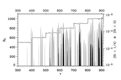
Figure 4: Time evolution of $R_{\lambda}$ (solid line) and the volume fraction of the domain with local $Ri<0.25$ (filled grey area) and with local $Ri<0$ (filled black area). There was no occurrence of $Ri<0.25$ for $0<\tau<300$.

A further transition, for $R_{\lambda}\approx 700$, is evident in local violations of the inviscid gravitational stability critical value of $Ri=0.0$ (Fig. 4). Finally, we see yet another transition for $R_{\lambda}\approx 900$, evident in the growth of vertical kinetic energy, $E_{z}$ (Fig. 3). Interestingly, throughout all these transitions, the principal measures of the internal-wave energy, $E_{w}$ and $E_{p}$, show little change relative to the vortical-mode energy, $E_{v}$. Since $E_{v}$ itself remains reasonably constant with time and its horizontal spectrum $\Phi_{v}(k_{h})$ maintains a similar shape and magnitude at low wavenumbers, we conclude that pancake motions are indeed persistent throughout the $R_{\lambda}$ range we have been able to explore, even though the structure and intensity of the flow changes substantially at high wavenumbers, in the horizontally uniform vertical shear, and in the vertical velocity.

III.1 Growth of the Vertical Shear Component

In Fig. 3 the vortical energy is nearly steady over the entire simulation. The wave energy is more variable, but on average it is steady as $R_{\lambda}$ increases. However, the shear energy is a growing function of time. It represents an inverse horizontal cascade of kinetic energy into $k_{h}=0$. The intensity of the inverse cascade of shear energy is probably a function of the location of the energy peak in the horizontal direction; in the present case, the forcing is imposed at $k_{h}=1$, and a substantial part of the energy is transformed into pure vertical shear. To assess the degree of equilibration for this inverse cascade, two additional simulations are made. Both start from the primary simulation and thereafter hold $R_{\lambda}$ constant for several hundred turnover times, but their starting $(\tau,\ R_{\lambda})$ values differ. Fig. 5 shows that $E_{s}$ does indeed

Figure 5: History of $R_{\lambda}(t)$ (solid lines) and $E_{s}(t)$ for three simulations. The primary simulation (with a dashed line for its $E_{s}$) has an increasing Reynolds number by steps of 100 from 200 to 1000, and the second and third simulations have constant Reynolds numbers of $R_{\lambda}=300$ (dash-dotted line) and $R_{\lambda}=500$ (dotted line), starting from the primary simulation at $\tau=200$ and $\tau=400$, respectively.

equilibrate over a period of less than 100 turnover times at a level that increases systematically with $R_{\lambda}$.

This growth of shear kinetic energy has been seen previously when the Froude number is below a critical value smith02 . For the alternative Froude number defined by $Fr_{s}=(\epsilon\,{k_{v}^{o}}^{2})^{1/3}/N)$, our simulations have a value of approximately 0.025, more than an order of magnitude below the identified critical value of 0.42. In this previous study, the shear kinetic energy did not equilibrate even after more than 1000 turnover times. This may be due to its reliance on hyper-diffusion in all directions that exerts only a weak damping on the shear component.

III.2 Onset of Overturning Motions

Overturning occurs when an unstable shear layer rolls up, pulling high-density fluid above low-density fluid. This instability can occur in a fairly localized way. Its occurrence is detected with the local $Ri$ defined in eq. (1), and an indication of the overturning instability is a negative $Ri$ value. Because of the Miles-Howard condition, we can expect that this Kelvin-Helmholtz instability only occurs in regions where $Ri$ is initially less than $0.25$. The history of the fraction of the domain with the local $Ri$ below 0.25 is shown in Fig. 4. More events with $Ri<0.25$ happen as $R_{\lambda}$ increases, although they evidently remain intermittent. The regime of overturning events first appears at $R_{\lambda}=700$ ($\tau\simeq 535$). Even at the highest $R$ value, only a small fraction of the domain is actively overturning at any time, less than 0.7%. The Probability Density Function (PDF) for $Ri$ shows that most of the domain remains far away from overturning, with only a small tail in the PDF that extends to small and negative $Ri$ values. Because of the intermittency, long averaging periods are required for stable statistics. Nevertheless, we can say that there is a well determined value of $R$ for the onset of overturning events. To demonstrate this, the regime just before the first overturning event in the primary simulation ($R_{\lambda}=500$) is integrated over a longer period (250 turnover times), and no overturning occurs despite several events with $Ri<0.25$. To characterize more precisely the critical $Ri$ for instability, we follow the history of the global minimum in local $Ri$ (Fig. 6).

Figure 6: History of the global minimum value of local $Ri$ for the primary simulation. The ordinate scale is split into three intervals to see both large and small values on the same plot. Whenever the minimum $Ri$ drops below about 0.02, it continues to develop into overturning in the density profile (i.e., min[Ri] $<$ 0); this first occurs around $\tau\simeq 400$.

The minimum $Ri$ value that does not immediately lead to local overturning is $Ri\simeq 0.02$. This value is a bit smaller but of the same order of magnitude than the values computed by Gage gage71 for simple shear flows.

The spatial distribution of small $Ri$ events is organized into thin sheets with large vertical shear in the horizontal velocity. An example of a region with a negative vertical density gradient is shown Fig. 7.

Figure 7: Instantaneous isolines of vertical density gradient at $\tau=741$ ($R_{\lambda}=900$) for two perpendicular slices of the whole domain at $z=cte$ (upper graph) and $y=cte$ (lower graph) .

The vertical size of this region is very thin (a few grid cells) even though its horizontal size at this time ($\simeq 2\pi/3$) is not much smaller than to the domain size. An intense vertical velocity is associated with domain of negative vertical density gradient (Fig. 8), but the present simulation has only a

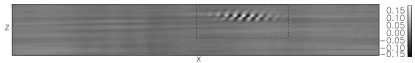
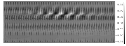
Figure 8: Vertical slice (same than in Fig. 7) of vertical velocity at $\tau=741$ ($R_{\lambda}=900$) (upper graph) and a zoom of the region of intense vertical velocity with the projection of velocity vectors (lower graph) .

marginally adequate resolution to expose the convective overturning events.

Fig. 9 shows the spectra for the energy components

Figure 9: Energy spectra with respect to horizontal and vertical wavenumbers at $\tau=521$ ($R_{\lambda}=700$) (upper graph) and $\tau=741$ ($R_{\lambda}=900$) (lower graph) for the primary simulation. The local energy peaks at $\tau=741$ for $40<k_{h}<60$ are an indication of one or several overturning events($Min[Ri]>0$).

at $\tau=521$, before any overturning occurs. The spectra with respect to horizontal wavenumber are very steep, with a slope close to $k_{h}^{-5}$ for $\Phi_{v}$, and the shape does not vary much with $R_{\lambda}$ in this stably stratified regime without overturning. The onset of the overturning instability does not seem to affect significantly the overall level of wave and vortical energy (Fig. 3). However, the overturning events are easily identifiable as a peak in the horizontal spectra at $\tau=741$ (Fig. 9). The peak is located at the horizontal scale $L_{h}\simeq 2\pi/50$ that matches the typical vertical scale, $L_{v}$. At this particular time, the instability is localized in a single region of the domain.

The energy at the largest horizontal scales is not affected by the overturning instabilities that are localized in both space and time. In Fig. 10,

Figure 10: Comparison of vortical (upper graph) and wave (lower graph) energy spectra with respect to horizontal and vertical wavenumbers for four different Reynolds number. Each spectrum is an average over more than 200 times for each $R_{\lambda}$. The horizontal spectra are very similar at large horizontal scales but differ at small scales ($k_{h}>10$). The situation is different in the vertical spectra, where the typical scale decreases with $R_{\lambda}$.

time-averaged vortical-energy spectra are compared for four values of $R_{\lambda}$. The horizontal spectra are very similar up to the typical scales of the overturnings. However, at both finer horizontal scales and at all vertical scales finer than the forcing scale, the spectrum amplitude increases systematically with $R_{\lambda}$. At the constant, small $Fr$ value in this simulation, the vertical spectrum slope becomes quite shallow as $R_{\lambda}$ increases.

III.3 Growth of Large-Scale Vertical Motions

The energy histories in Fig. 3 expose another transition at an even larger $R_{\lambda}\simeq 900$, viz., the systematic growth of vertical kinetic energy $E_{z}$. Inspection of the vertical energy spectrum reveals that the growth of $E_{z}$ after $\tau=700$ occurs principally at $k_{v}=0$ (Fig. 11).

Figure 11: Evolution in time of the total vertical energy (thin line) and the vertical energy at the zero vertical mode (thick line) for the primary simulation (parameters of Fig. 1). The component of the zero vertical mode is several order of magnitude smaller than the total vertical energy for $\tau<700$ and become the dominant mode for $\tau>800$

This mode of instability is reminiscent of the “negative-viscosity instability” observed in a Kolmogorov flow dubrulle91b , further investigated by Dubrulle & Frisch dubrulle91a with a multi-scale analysis. This analysis shows that a parallel flow with a small transverse scale develops a negative-viscosity instability to large-scale perturbations in the transverse direction when the viscosity becomes less than the RMS value of the streamfunction of the primary flow. In our simulation, it is difficult to test precisely this criterion of instability because the streamfunction is ill-defined. Crudely, we can expect an instability of this type when $\nu<\Phi_{s}(\ell_{v})^{1/2}\ell_{v}$, where $\ell_{v}$ is the scale of the vertical shear and $\Phi_{s}(\ell_{v})$ is the shear energy at this scale. In our simulation this relation is satisfied on average for $\tau>700$ if $2\pi/\ell_{v}>80$. This scale is comparable in magnitude with the typical vertical wavenumber $2\pi/L_{v}\simeq 50$. However, due to the complexity of the forced stratified flow, it is difficult to prove the nature of this instability pending more apt stability analyses.

IV Summary and Discussion

In our simulations of forced, equilibrium, stratified turbulence, we see behaviors somewhat different from many previous studies of decaying stratified turbulence that were not able to sustain a large value of the Reynolds number, $R$. Most often the criteria for the occurrence of pancake vortices and suppression of overturning motions (i.e., Kelvin-Helmholtz and gravitational stability) have been linked to the stratification $N$ but rarely to $R$. Indeed, we find that the stability of a solution is mainly controlled by two parameters with opposite effects on stability: increasing N (decreasing $Fr$) leads to a more stable solution and decreasing $\nu$ (increasing $R$) has the opposite effect. For a fixed low value of $Fr$, we follow an experimental path of increasing $R$ far enough to detect several regime transitions beyond the familiar one of stable pancake vortices. One transition is to the intermittent occurrence of regions with small or negative $Ri$. This refutes previous arguments lilly83 ; mcwilliams85 that stratified turbulence remains stable with uniformly small local values of $Fr$ at large $R$ and with uniformly cyclostrophic, hydrostatic diagnostic momentum balances. This transition may plausibly be associated with inviscid Kelvin-Helmholtz and ensuing gravitational instabilities of the pancake vortices, although in our simulations the viscous effects on the unstable scales are significant. Nevertheless, the pancake vortices continue to be the energetically dominant component of the turbulence even up to the highest $R$ values examined here, and visualizations of the large-scale potential vorticity field (not shown) show little change in spatial structure with $R_{\lambda}$.

Two other transitions to large-scale motions other than pancake vortices do occur: a first one to growth of the shear kinetic energy at zero horizontal wavenumber and a second one to growth of vertical kinetic energy with its spectrum peak at zero vertical wavenumber for large $R$. The former has been seen previously in stratified turbulence smith02 , and the latter may be associated with negative-viscosity instability seen previously in unstratified shear flow dubrulle91b . Each of these large-scale transitions may be interpreted as an inverse energy cascade. However, they behavior is strongly constrained by the domain size in our simulations where the forcing is imposed at the gravest finite wavenumbers. We will explore beyond this limitation in future reports.

In this paper we choose to focus on simulations at very small Froude number, and we are able to reach a Reynolds number high enough to destabilize the pancake vortices in several ways. This leads us to advance the following proposition about the nature of equilibrium stratified turbulence: for any Froude number, no matter how small, there are Reynolds numbers large enough so that a sequence of transitions to non-pancake motions will always occur, and, conversely, for any Reynolds number, no matter how large, there are Froude numbers small enough so that these transitions are suppressed. Obviously, this hypothesis warrants further testing, as do our provisional interpretations of the dynamical nature of the transitions.

References

- (1) A. Craya. Contribution à l’analyse de la turbulence associée à des vitesses moyennes. Technical Report 345, Publ. Sci. Tech. Ministère de l’air, 1958.
- (2) B. Dubrulle and U. Frisch. Eddy viscosity of parity-invariant flow. Phys. Rev. A, 43:5355–5364, 1991.
- (3) B. Dubrulle, U. Frisch, and M. Hénon. Low-viscosity lattice gases. J. Stat. Phys., 59:1187–1226, 1991.
- (4) P. F. Embid and A. J. Majda. Low froude number limiting dynamics for stably stratified flow with small or finite rossby number. Geophys. Astrophys. Fluid Dyn., 87:1–50, 1998.
- (5) A. M. Fincham, T. Maxworthy, and G. R. Spedding. Energy dissipation and vortex struture in freely decaying stratified turbulence. Dyn. Atmos. Ocean, 23:155–169, 1996.
- (6) K. S. Gage. The effect of stable stratification on the stability of viscous parallel flows. J. Fluid Mech., 47:1–20, 1971.
- (7) F. S. Godeferd and C Cambon. Detailed investigation of energy transfers in homogeneous stratified turbulence. Phys. Fluids, 6:2084–2100, 1994.
- (8) J. R. Herring and Métais O. Numerical experiments in forced stably stratified turbulence. J. Fluid Mech., 202:97–115, 1989.
- (9) L. N. Howard. Note on a paper of John W. Miles. J. Fluid Mech., 10:509–512, 1961.
- (10) Y. Kimura and J. R. Herring. Diffusion in stably stratified turbulence. J. Fluid Mech., 328:253–269, 1996.
- (11) M. P. Lelong. Internal wave–vortical mode interactions in strongly stratified flows. J. Fluid Mech., 232:1–19, 1991.
- (12) D. K. Lilly. On the computational stability of numerical solutions of time-dependent, nonlinear, geophysical fluid dynamic problems. Mon. Wea. Rev., 93:11, 1965.
- (13) D. K. Lilly. Stratified turbulence and the mesoscale variability of the atmosphere. J. Atmos. Sci., 40:749–761, 1983.
- (14) A. J. Majda and M. G. Shefter. Elementary stratified flows with instability at large Richardson number. J. Fluid Mech., 376:319–350, 1998.
- (15) J. C. McWilliams. A note on a uniformly valid model spanning the regimes of geostrophic and isotropic, stratified turbulence: balanced turbulence. J. Atmos. Sci., 42:1773–1774, 1985.
- (16) O. Métais and J. R. Herring. Numerical simulation of freely evolving turbulence in stably stratified fluids. J. Fluid Mech., 202:117–148, 1989.
- (17) J. W. Miles. On the stability of heterogeneous shear flows. J. Fluid Mech., 10:496–508, 1961.
- (18) H. Peters, M. C. Gregg, and J. M. Toole. On the parameterization of equatorial turbulence. J. Geophys. Res., 93:1199–1218, 1988.
- (19) J. J. Riley and M.-P. Lelong. Fluid motion in the presence of stong stratification. Annu. Rev. Fluid Mech., 32:613–657, 2000.
- (20) L. M. Smith and F. Waleffe. Generation of slow, large scales in forced rotating, stratified turbulence. J. FLuid Mech., 451:145–168, 2002.
- (21) C. Staquet and F. S. Godeferd. Statistical modelling and direct numerical simulations of decaying stably stratified turbulence. part 1. flow energetics. J. Fluid Mech., 360:295–340, 1998.
- (22) A. Vincent and M. Meneguzzi. The spatial structure and statistical properties of homogenous turbulence. J. Fluid Mech., 225:1–20, 1991.
- (23) J. Werne and D. C. Fritts. Stratified shear turbulence: Evolution and statistics. Geophys. Research Lett., 26:439–442, 1999.
- (24) C. T. Yap and C. W. van Atta. Experimental studies of the development of quasi-two-dimensional turbulence in stably stratified fluid. Dyn. Atmos. Oceans, 19:289–323, 1993.