Non-stationary Spectra of Local Wave Turbulence

Abstract

The evolution of the Kolmogorov-Zakharov (K-Z) spectrum of weak turbulence is studied in the limit of strongly local interactions where the usual kinetic equation, describing the time evolution of the spectral wave-action density, can be approximated by a PDE. If the wave action is initially compactly supported in frequency space, it is then redistributed by resonant interactions producing the usual direct and inverse cascades, leading to the formation of the K-Z spectra. The emphasis here is on the direct cascade. The evolution proceeds by the formation of a self-similar front which propagates to the right leaving a quasi-stationary state in its wake. This front is sharp in the sense that the solution remains compactly supported until it reaches infinity. If the energy spectrum has infinite capacity, the front takes infinite time to reach infinite frequency and leaves the K-Z spectrum in its wake. On the other hand, if the energy spectrum has finite capacity, the front reaches infinity within a finite time, ${t^{*}}$, and the wake is steeper than the K-Z spectrum. For this case, the K-Z spectrum is set up from the right after the front reaches infinity. The slope of the solution in the wake can be related to the speed of propagation of the front. It is shown that the anomalous slope in the finite capacity case corresponds to the unique front speed which ensures that the front tip contains a finite amount of energy as the connection to infinity is made. We also introduce, for the first time, the notion of entropy production in wave turbulence and show how it evolves as the system approaches the stationary K-Z spectrum.

I Introduction and Motivation

Wave turbulence is concerned with the statistical description of an infinite sea of dispersive waves, which are weakly coupled by nonlinear interactions and maintained away from equilibrium by interaction with sources and sinks of energy. The theory has found practical application in many branches of physics including the description of surface waves on fluid interfaceshasselmann1962 ; hasselmann1963 ; benney67 ; zakharov66 , Alfven wave turbulence in astrophysical plasmas galtier2000 ; ng96 , nonlinear opticsdyachenko92 and acousticsnewell71 ; zakharov70 to name a few.

The central quantity of theoretical interest is the spectral wave action density, $n_{\bf k}$, which describes how the excitations in the system are distributed among different wave-vectors, ${\bf k}$. Under fairly weak assumptionsnewell2001 , the long time behaviour of $n_{\bf k}$ is given by an equation known as the wave kinetic equation. For a system dominated by four wave interactions this equation takes the form,

$$\frac{\partial n_{\bf k}}{\partial t}=4\pi\int\left|T_{{\bf k}{\bf k}_{1}{\bf k}_{2}{\bf k}_{3}}\right|^{\ 2}\ {\mathcal{F}}_{4}\left[n_{\bf k}\right]\delta({\bf k}\!+\!{\bf k}_{1}\!-\!{\bf k}_{2}\!-\!{\bf k}_{3})\ d{\bf k}_{1}d{\bf k}_{2}d{\bf k}_{3},$$ (1)

where

$${\mathcal{F}}_{4}\left[n_{\bf k}\right]=n_{\bf k}n_{{\bf k}_{1}}n_{{\bf k}_{2}}n_{{\bf k}_{3}}\left(\frac{1}{n_{\bf k}}+\frac{1}{n_{{\bf k}_{1}}}-\frac{1}{n_{{\bf k}_{2}}}-\frac{1}{n_{{\bf k}_{3}}}\right)\delta(\omega_{{\bf k}}\!+\!\omega_{{\bf k}_{1}}\!-\!\omega_{{\bf k}_{2}}\!-\!\omega_{{\bf k}_{3}}).$$ (2)

Equation (1) is the analogue for waves of the Boltzmann equation of classical statistical mechanics. In many applications, $\omega_{\bf k}$ and $T_{{\bf k}{\bf k}_{1}{\bf k}_{2}{\bf k}_{3}}$ are homogeneous functions of their arguments. Their degrees of homogeneity shall be denoted by $\alpha$ and $\gamma$ respectively. Under rescaling, ${\bf k}\to\lambda{\bf k}$, they transform as follows :

$$\omega_{\lambda{\bf k}}=\lambda^{\alpha}\omega_{\bf k}$$ (3)

$$T_{\lambda{\bf k}\lambda{\bf k}_{1}\lambda{\bf k}_{2}\lambda{\bf k}_{3}} = \lambda^{\gamma}T_{{\bf k}{\bf k}_{1}{\bf k}_{2}{\bf k}_{3}}.$$ (4)

It was shown by Zakharovzakharov in the 60’s that if the energy sources and sinks are separated by an “inertial range”, equation (1) has exact isotropic steady state solutions,

$$n_{\bf k} = c_{1}P^{1/3}k^{-(2\gamma+3d)/3}$$ (5)

$$n_{\bf k} = c_{2}Q^{1/3}k^{-(2\gamma+3d-1)/3},$$ (6)

which carry constant fluxes of conserved densities, in this case energy flux, $P$, or wave action flux, $Q$, between sources and sinks. These steady state spectra are the direct analogues of the direct and inverse cascades in hydrodynamic turbulence and are referred to as Kolmogorov-Zakharov (K-Z) spectra. They have been well observed experimentally in a variety of contexts.

In 1991 Falkovich and Shafarenkofalkovich91 addressed the question of how the K-Z spectrum is set up in time if $n_{\bf k}$ is initially compactly supported in wave-vector space. They used a self-similar solution of (1) and an assumption that, for the direct cascade, the total energy increases linearly in time, to show that (5) is set up by a nonlinear front which propagates towards $k=\infty$ and leaves the $k^{-(2\gamma+3d)/3}$ spectrum in its wake.

However subsequent numerical simulations of the kinetic equation for Alfven wave turbulence performed by Galtier et al. galtier2000 suggested that the development of the K-Z spectrum may proceed by a different route. For the Alfven wave system, the K-Z energy spectrum has finite energy capacity, meaning that on the K-Z spectrum, $\int E({\bf k})\ d{\bf k}<\infty$. This implies that the nonlinear front must reach $k=\infty$ within a finite time, ${t^{*}}$. They noticed that the spectrum in the wake of the front was significantly steeper than the K-Z value for times less than the singular time, ${t^{*}}$, and that the K-Z spectrum then developed from right to left after the front reached $k=\infty$. Other work by Pomeau et al.pomeau2001 on the inverse cascade in the Nonlinear Schrodinger equation suggested that there might be anomalous quasi-stationary spectra associated with non-stationary solutions of kinetic equations. However no-one has yet made a specific attempt to search for them.

One of the challenges in far-from-equilibrium systems is to understand the means by which stationary states are reached and to ask if there are functionals analogous to the entropy in equilibrium systems. What we will show is that while the entropy, which for wave turbulence is formally (see for example aucoin1971 )

$$S=\int\ln n_{\bf k}\,d{\bf k},$$ (7)

is not well defined on the steady state solutions, spectra (5) and (6), its production rate is. We find that for $0<t<{t^{*}}$, when the spectrum in the wake of the front is steeper than the K-Z spectrum, the entropy production is positive. At ${t^{*}}$ the connection to ${\bf k}=\infty$ is made and energy is no longer a conserved quantity. For $t>{t^{*}}$, the K-Z spectrum is established via a front which travels back from ${\bf k}=\infty$. During this stage, the entropy production rate, while still positive, gradually decreases and asymptotes to zero, its value on the exact K-Z spectrum. We conjecture that this scenario, established in this paper for the differential approximation to the kinetic equation, (1), will be widely valid for finite capacity non-equilibrium systems, including three-dimensional hydrodynamic turbulence at large Reynolds numbers.

This leads us to the topic of this article. We have made an extensive study of the non-stationary solutions of the so-called differential kinetic equation of local wave turbulence. This model equation is obtained from (1) under the assumption that the interaction co-efficient, $T_{{\bf k}{\bf k}_{1}{\bf k}_{2}{\bf k}_{3}}$ is strongly localised in ${\bf k}{\bf k}_{1}{\bf k}_{2}{\bf k}_{3}$ space. It has the advantage of replacing the integro-differential kinetic equation with a PDE. We find that the qualitative bahaviour observed by Galtier et al is present in this model in the finite capacity case. Since we are dealing with a PDE, we can go a lot further in terms of understanding.

The organisation of the article is as follows. In section II we introduce the differential kinetic equation and describe a few of its properties which make it a good model of wave turbulence. We also introduce exact expressions for the fluxes of energy ($P$), the flux of particles ($Q$), and the entropy production rate in terms of its flux ($R$) and its bulk production rate ($T$). The latter is always positive definite. We calculate each of these quantities on the algebraic solutions, $n_{\bf k}\propto k^{-\alpha x}$. Section III contains the details of some numerical simulations of the PDE. These simulations suggest that the nonlinear front is “sharp” in the sense that $n_{\bf k}$ remains compactly supported for $t<{t^{*}}$. There is a singularity, a divergence in the second derivative in fact, at the front tip between the regions $n_{\bf k}=0$ and $n_{\bf k}>0$. Next, in section IV, we construct a family of self-similar solutions of the differential kinetic equation which are parameterised by a single free parameter. This free parameter can be interpreted as the asymptotic slope behind the front. Following that, in section V, we use this self-similarity analysis to formulate a hypothesis which we call the critical front speed hypothesis. This hypothesis is based on physical arguments and allows us to select a critical value, $x_{c}$, for the asymptotic slope, given by

$$x_{c}=x_{0}+\frac{2\gamma-3\alpha}{12\alpha},$$ (8)

where $x_{0}$ denotes the usual K-Z exponent for the direct cascade. This formula is well supported by our numerical simulations. In our conclusion, we attempt to make a connection with entropy production arguments. Two appendices are provided. In the first, we analyse the mathematical structure of the similarity equation and try to understand how the critical slope is related to the solution trajectories of the underlying ordinary differential equation. The second appendix contains a brief outline of the numerical methods used.

II The Differential Kinetic Equation

We begin by briefly discussing the origin of the differential kinetic equation. Assuming that the wave-action spectrum rapidly becomes isotropic, and averaging over angles, we can make a transformation from $d$-dimensional wave-vector space to frequency space,

$$\frac{\partial N_{\omega}}{\partial t}=\int S_{\omega\omega_{1}\omega_{2}\omega_{3}}\ {\mathcal{F}}_{4}\left[n_{\omega}\right]\ d\omega_{1}d\omega_{2}d\omega_{3}$$ (9)

where

$$S_{\omega\omega_{1}\omega_{2}\omega_{3}}=4\pi\!\int\!\!\left|T_{kk_{1}k_{2}k_{3}}\right|^{\ 2}\delta({\bf k}\!+\!{\bf k}_{1}\!-\!{\bf k}_{2}\!-\!{\bf k}_{3})\ (kk_{1}k_{2}k_{3})^{d-1}\frac{dk}{d\omega}\frac{dk_{1}}{d\omega_{1}}\frac{dk_{2}}{d\omega_{2}}\frac{dk_{3}}{d\omega_{3}}\ d\Omega$$ (10)

and $N_{\omega}$ is defined by requiring that

$$\int\phi(\omega)N_{\omega}d\omega=\int\phi(\left|{\bf k}\right|^{\alpha})\ n_{\bf k}d{\bf k},$$ (11)

for any test function, $\phi$. Here the volume element $d\Omega$ represents integration over the angular variables in ${\bf k}_{1}{\bf k}_{2}{\bf k}_{3}$ space and the wave-vector moduli are related to the frequency via the dispersion relation,

$$\omega_{k}=ck^{\alpha}.$$ (12)

If we assume that the interaction coefficient, $T_{{\bf k}{\bf k}_{1}{\bf k}_{2}{\bf k}_{3}}$ is strongly local in ${\bf k}{\bf k}_{1}{\bf k}_{2}{\bf k}_{3}$ space then (9) can be approximated by a differential equation dyachenko92 ,

$$\frac{\partial N_{\omega}}{\partial t}=I\frac{\partial^{2}}{\partial\omega^{2}}\left(\omega^{s}n_{\omega}^{4}\frac{\partial^{2}}{\partial\omega^{2}}\left(\frac{1}{n_{\omega}}\right)\right),$$ (13)

where

$$n_{\omega}(t) = n(k(\omega),t)$$ (14)

$$s = 3x_{0}+2$$ (15)

$$x_{0} = \frac{2\gamma+3d}{3\alpha}.$$ (16)

$I$ is a pure number which comes from the angular integrations in (10). This equation is called the differential kinetic equation.

The local approximation leading to the differential kinetic equation, (13), is rather drastic and is not justified for many of the physical applications of weak turbulence. Nonetheless, it retains many of the qualitative features of the full kinetic equation, (9). It provides an excellent model in the context of which these features can be easily studied. In particular, the differential kinetic equation respects the conservation laws embodied within its integro-differential precursor, namely the conservation of the total energy,

$$E=\int\omega N_{\omega}\ d\omega,$$ (17)

and the total number of particles,

$$N=\int N_{\omega}\ d\omega.$$ (18)

It also preserves the scaling and homogeneity properties of the kinetic equation. Consequently, the pure scaling solutions of the kinetic equation, the equilibrium thermodynamic spectra and the non-equilibrium K-Z spectra, are also solutions of the differential kinetic equation. These solutions are of the form $n_{\omega}=c\omega^{-x}$ where $x$ takes one of the following values:

$$x=1,\hskip 14.22636ptx=0,\hskip 28.45274pt\mbox{\rm(thermodynamic)}$$

or

$$x=\frac{2\gamma+3d}{3\alpha},\hskip 14.22636ptx=\frac{2\gamma+3d-\alpha}{3\alpha},\hskip 28.45274pt\mbox{\rm(K-Z).}$$

It is convenient to define

$${\mathcal{K}}\left[n_{\omega}\right]=\omega^{3x_{0}+2}n_{\omega}^{4}\frac{\partial^{2}}{\partial\omega^{2}}\left(\frac{1}{n_{\omega}}\right).$$ (19)

The two conservation laws can be written as continuity equations :

$$\frac{\partial N_{\omega}}{\partial t}-\frac{\partial Q}{\partial\omega} = 0$$ (20)

$$\frac{\partial E_{\omega}}{\partial t}+\frac{\partial P}{\partial\omega} = 0,$$ (21)

where

$$Q=\frac{\partial{\mathcal{K}}}{\partial\omega}$$ (22)

is the local flux of particles,

$$P={\mathcal{K}}-\omega\frac{\partial{\mathcal{K}}}{\partial\omega}$$ (23)

is the local flux of energy and

$$E_{\omega}=\omega N_{\omega}$$ (24)

is the energy density if frequency space. Note that $P$ is defined to be positive when energy flows to the right in $\omega$ space and $Q$ is positive when particles flow to the left.

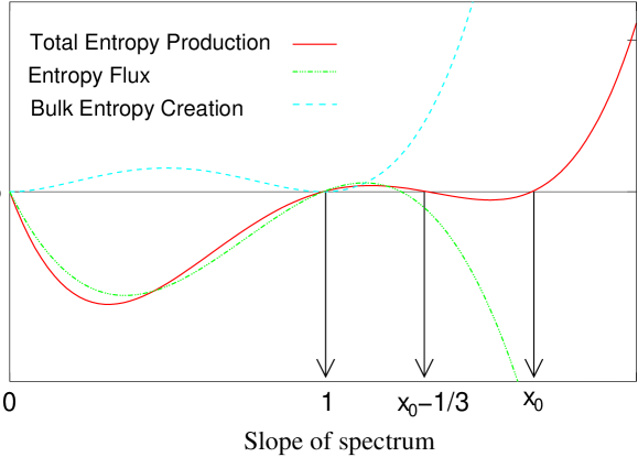
Figure 1: Plot of the bulk entropy production, $T$, the entropy flux, $R$, and the total entropy production, $\dot{S}$, as a function of the exponent, $x$, of the spectrum for power law spectra, $n_{\omega}=c\omega^{-x}$.

The entropy, $S$, of a wave system is formally $\int\ln n_{\bf k}\,d{\bf k}$. The production rate,

$$\frac{dS}{dt}=\frac{d}{dt}\,\int\ln n_{\bf k}\,d{\bf k}=\int\frac{1}{n_{\omega}}\,\frac{dN_{\omega}}{dt}\,d\omega,$$ (25)

can readily be calculated to be

$$\dot{S}=-\frac{\partial R}{\partial\omega}+T.$$ (26)

The entropy flux, $R$, which is positive for entropy flow to large wave-numbers, is

$$R=-\frac{Q}{n_{\omega}^{2}}\frac{\partial}{\partial\omega}(\omega n_{\omega})-\frac{P}{n_{\omega}^{2}}\frac{\partial n_{\omega}}{\partial\omega}$$ (27)

and the local bulk entropy production rate, $T$, is

$$T=I\omega^{3x_{0}+2}n_{\omega}^{4}\left(\frac{\partial^{2}}{\partial\omega^{2}}\left(\frac{1}{n_{\omega}}\right)\right)^{2}.$$ (28)

Note that $T$ is positive definite and zero on the thermodynamic solution, $n_{\omega}=\tau/(\omega-\mu)$ , $\tau$ being the temperature and $\mu$ the chemical potential. Indeed if the system were isolated, say on the interval $\omega_{1}<\omega<\omega_{2}$, and $P$, $Q$ and $R$ were identically zero, then the usual principles of equilibrium systems would apply.

On the solution $n_{\omega}=c\omega^{-x}$, the quantities $K$, $Q$, $P$, $R$, $T$ and $-\frac{\partial R}{\partial\omega}+T$ are calculated. They are:

$$K = I\,c^{3}\omega^{3x_{0}-3x}x(x-1)$$ (29)

$$Q = 3Ic^{3}x(x-1)(x_{0}-x)\,\omega^{3x_{0}-3x-1}$$ (30)

$$P = 3Ic^{3}x(x-1)(x-(x_{0}-{\scriptstyle\frac{1}{3}}))\,\omega^{3x_{0}-3x}$$ (31)

$$T = c^{2}\,I\,x^{2}(x-1)^{2}\,\omega^{3x_{0}-2x-2}$$ (32)

$$R = 3c^{2}\,I\,x(x-1)(x_{0}-{\scriptstyle\frac{4}{3}}x)\,\omega^{3x_{0}-2x-1},$$ (33)

$$\dot{S} = -\frac{\partial R}{\partial\omega}+T=9c^{2}\,I\,x(x-1)(x-x_{0})(x-(x_{0}-{\scriptstyle\frac{1}{3}}))\,\omega^{3x_{0}-2x-2}.$$ (34)

Similar expressions, which have the same zeros (as functions of $x$) obtain for the case when the differential approximation is replaced by the full collision integral. In particular, we note that the entropy production rate is always positive (we assume $x_{0}>4/3$) for $1<x<x_{0}-1/3$ and for $x>x_{0}$, the K-Z exponents for particles and energy respectively. The relevant functions are plotted in figure 1. For $x_{0}-1/3<x<x_{0}$, the entropy production rate is negative. This corresponds to a situation when the particle flux is building a condensate state pomeau2001 .

III Numerical Observations of Non-stationary Spectra

Let us now turn our attention to non-stationary solutions of (13). In particular we are interested in how the K-Z spectra are set up if we begin from an initial condition which is compactly supported at low frequencies. Early work on this question focussing on the direct cascade by Falkovich and Shafarenko falkovich91 suggested that the K-Z spectrum is set up by a nonlinear front which propagates to the right leaving the K-Z spectrum in its wake. Recent numerical studies by Galtier et al galtier2000 suggest that this problem is more subtle. They found that in the case where the K-Z energy spectrum has finite capacity, the approach to the steady state proceeds by a different mechanism. For this system the nonlinear front reaches infinite frequency within a finite time, $t^{*}$. They found that the quasi-stationary spectrum in the wake of this front was actually steeper than the K-Z spectrum. The K-Z spectrum was then set up from right to left after the front reached infinity.

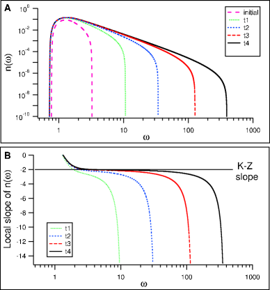
Figure 2: Time evolution of the spectrum and the local slope for the parameter values $\alpha=0.5,\gamma=0,d=1$. The logarithmic scales are to base 10.

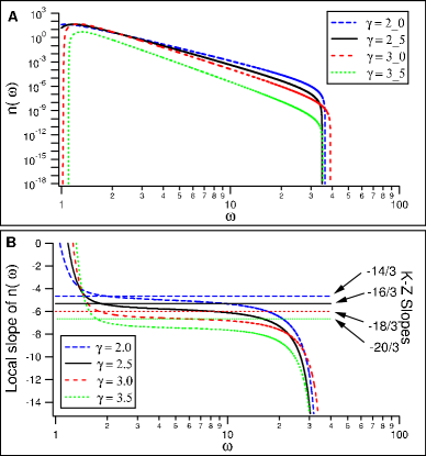
Figure 3: Snapshots of the non-stationary spectrum for a range of different values of the parameter $\gamma$, keeping $\alpha=1/2$ and $d=1$. The logarithmic scales are to base 10.

We investigated whether there was evidence of this behaviour in the solutions of the differential kinetic equation. We solved the differential kinetic equation numerically and followed the evolution from an initial condition compactly supported at low frequencies. The results presented in this section were obtained by allowing the initial data to decay freely in the absence of forcing or damping. Some details of the numerical methods used are contained in appendix B.

Let us first consider the situation in which the energy spectrum has infinite capacity, $2\gamma<3\alpha$. Figure 2 shows a sequence of snapshots of $n_{\omega}$ and the local slope at successive times for a system with parameter values $\alpha=0.5,\gamma=0,d=1$. We conclude that the slope tends to the K-Z value far behind the front in agreement with previous expectations. The K-Z spectrum is set up asymptotically in time from the left of the window of transparency to the right.

Now consider what happens when we increase the value of $\gamma$ and bring the system into the finite capacity regime. Figure 3 shows the absolute value of the local slope of $n_{\omega}$ at similar stages in the evolution for a sequence of values of $\gamma$ in the finite capacity regime. $\gamma$ takes the values 2.0, 2.5, 3.0 and 3.5. Visually, it is clear that as $\gamma$ increases, the slope of the spectrum behind the front tends to a value which is increasingly steeper than the K-Z value. This observation is supported by fitting power law functions to the numerical data. The “best fit” slopes are presented in Table 1 along with the K-Z values for comparison. The slope given by equation (8) agrees well with the numerical observations. The time, $t^{*}$, required for the front to reach infinity depends both on the parameters $\gamma$ and $\alpha$ and on the initial energy distribution. We have not, in the present work, made any systematic attempt to understand this aspect of the problem.

$\gamma$	$x_{KZ}$	xnum	xc
2.0	-4.67	-5.12	-5.08
2.5	-5.33	-5.93	-5.92
3.0	-6.00	-6.67	-6.75
3.5	-6.67	-7.50	-7.58

Table 1: Numerical evidence for the anomaly. The table shows the values of the wake slopes obtained by fitting numerical data for a range of values of $\gamma$ in the finite capacity regime. These are to be compared to the K-Z values and the values of the critical slope obtained from equation (8) : $x_{c}=x_{KZ}+(2\gamma-3\alpha)/12\alpha$.

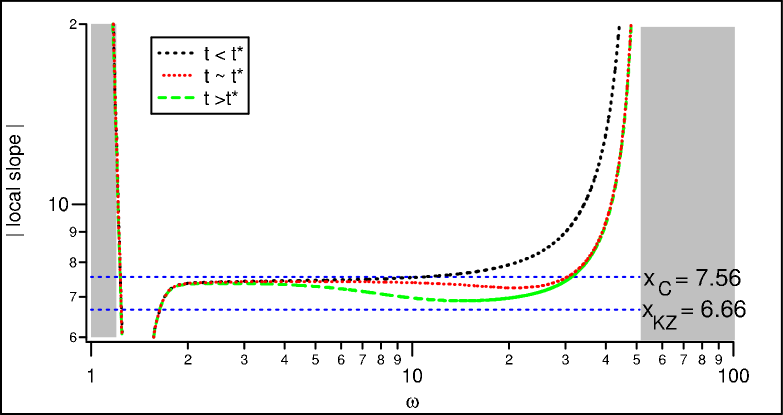
Figure 4: Log-log plot showing the initial stages of relaxation to the K-Z slope after the front reaches $\omega_{R}$. Parameter values are $\gamma=7/2$, $\alpha=1/2$ and $d=1$. The absolute value of the local slope is plotted as a function of frequency for three different times, just before ${t^{*}}$, approximately at ${t^{*}}$ and after ${t^{*}}$. There is a clear transition from the steeper slope, $x_{c}$, to the shallower $x_{KZ}$.

The next obvious question is that of how the system makes the transition from this quasi-steady anomalous regime to the K-Z spectrum which we know to be the final steady state. For finite capacity systems this transition begins once the front reaches infinity. Clearly we cannot easily treat the divergence of the front numerically. Instead we allow the front to propagate into a regime of strong damping to the right of the window of transparency. This damping region is intended to mimic the energy sink role provided by the point $\omega=\infty$. Figure 4 shows the local slope of $n_{\omega}$ for successive times after the front reaches the dissipation region. The results of Figure 4 are for $\gamma=3.5$ where there is a significant difference of about 0.9 between the anomalous slope and the K-Z slope. We see that the system begins to relax towards the K-Z spectrum as soon as the dissipation scale is reached. Notice that the relaxation is occurring from right to left.

Another issue which is crucial to our explanation of the finite capacity anomaly is the structure of the front itself. From our numerical simulations we found that the front tip seems to be “sharp” in the sense that the spectral wave action density remains on compact support during the time evolution. Such sharp fronts have been known to exist in solutions of certain classes of nonlinear diffusion equations dating back to the work of Zel’dovich in the 50’s. zeldovich50 Subsequent work by Lacey et al. lacey82 showed that such fronts can be stationary, moving or exhibit waiting time behaviour where the tip remains stationary for a finite time before beginning to move.

Let us suppose that our system possesses a sharp tip located at ${\omega^{*}}(t)$ and

$$n(\omega,t)\left\{\begin{array}[]{ll}=0&\hskip 14.22636pt\mbox{for $\omega\geq{\omega^{*}}(t)$}\\ >0&\hskip 14.22636pt\mbox{for $\omega<{\omega^{*}}(t)$.}\end{array}\right.$$

To the left of ${\omega^{*}}(t)$, we look for a solution of equation (13) in the form of a power series,

$$n(\omega,t)=A(t)\sum_{i}a_{i}({\omega^{*}}(t)-\omega)^{m_{i}},$$ (35)

where the constants $a_{i}$ and the exponents $m_{i}$ are to be determined by expanding equation (13) around $\omega={\omega^{*}}(t)$ and substituting this representation for $n(\omega,t)$. The leading order term on the LHS is

$$A{\omega^{*}}^{\frac{d}{\alpha}-1}m_{0}a_{0}({\omega^{*}}-\omega)^{m_{0}-1}\frac{d{\omega^{*}}}{dt}.$$ (36)

The leading order term on the RHS is

$$A^{3}{\omega^{*}}^{s}m_{0}(m_{0}+1)(3m_{0}-2)(3m_{0}-3)a_{0}^{3}({\omega^{*}}-\omega)^{3m_{0}-4}.$$ (37)

Comparing powers of ${\omega^{*}}-\omega$ immediately yields $m_{0}=3/2$. We cannot fix the time dependence although we get the following relation between $A(t)$ and ${\omega^{*}}(t)$,

$${\omega^{*}}(t)^{\frac{d}{\alpha}-1}\frac{d{\omega^{*}}}{dt}=A^{2}(t){\omega^{*}}(t)^{s},$$ (38)

after choosing $a_{0}^{-2}=(m_{0}+1)(3m_{0}-2)(3m_{0}-3)$. The presence of a sharp tip and the structure

$$n(\omega,t)\sim A(t)a_{0}({\omega^{*}}(t)-\omega)^{3/2},$$ (39)

immediately behind the tip is well supported by our numerical simulations as shown in figure 5.

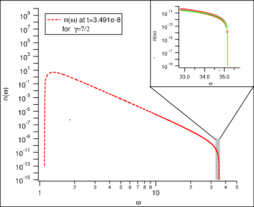
Figure 5: Inset shows a detailed view of the structure of the front tip seen in the evolution of a finite capacity spectrum. The parameter values are $\gamma=7/2$, $\alpha=1/2$ and $d=1$. The line is a least squares fit of the numerical data to the functional form $n(\omega)\sim A({\omega^{*}}-\omega)^{c}$ as suggested by equation (39). The fitted value of $c$ is 1.52.

IV Self-Similar Solutions of the Differential Kinetic Equation

To study non-stationary solutions of (13) analytically, make the following self-similarity ansatz for the form of the solution,

$$n_{\omega}(t)={\omega^{*}}(t)^{-x}\ F(\eta),$$ (40)

where the self-similar variable, $\eta$, is defined by

$$\eta=\frac{\omega}{{\omega^{*}}(t)}.$$ (41)

Under this change of variables the derivatives transform according to the relations,

$$\frac{\partial}{\partial t} = \dot{{\omega^{*}}}\left(\frac{\partial}{\partial{\omega^{*}}}-\eta{\omega^{*}}^{-1}\frac{\partial}{\partial\eta}\right)$$ (42)

$$\frac{\partial}{\partial\omega} = {\omega^{*}}^{-1}\frac{\partial}{\partial\eta},$$ (43)

and equation (13) can be rewritten as

$$A\ \eta^{\frac{d}{\alpha}-1}\left(-xF-\eta\frac{dF}{d\eta}\right)=\frac{d^{2}}{d\eta^{2}}\left(\eta^{s}F^{4}\frac{d^{2}}{d\eta^{2}}\left(\frac{1}{F}\right)\right),$$ (44)

where

$$A=\dot{{\omega^{*}}}\ {\omega^{*}}^{2x+d/\alpha-3x_{0}}.$$ (45)

Here $x_{0}=(2\gamma+3d)/3\alpha$ is the exponent of the K-Z energy spectrum. The free parameter, $x$, is the asymptotic slope of the spectrum far behind the front. This is because we assume that there exists a quasi-stationary regime far behind the front, which is a simple power law to leading order, $n_{w}\sim\omega^{-y}$. We must therefore have $y=x$ in order to cancel the time dependence from the leading order part of (40).

For a self-similar solution, $A$ must be time independent. We are interested in situations where the system has finite energy capacity and generates a singularity within a finite time which we shall denote by ${t^{*}}$. The appropriate solution of (45) describing such situations is

$${\omega^{*}}(t)=({t^{*}}-t)^{b}.$$ (46)

It is convenient to define

$$\kappa_{d}=\frac{2\gamma-3\alpha}{3\alpha}.$$ (47)

The direct cascade has infinite energy capacity for $\kappa_{d}<0$ and finite energy capacity for $\kappa_{d}>0$. Upon substitution of the form (46) into (45) it follows that

$$b = \left(2(x-x_{0})-\kappa_{d}\right)^{-1}$$ (48)

$$A = -b$$ (49)

We can also define

$$\kappa_{i}=\frac{2\gamma-\alpha}{3\alpha},$$ (50)

such that the inverse cascade has infinite particle capacity for $\kappa_{i}>0$ and finite particle capacity for $\kappa_{i}<0$. Equation (48) can be written in the equivalent form

$$b=\left(2(x-x_{0}+1/3)-\kappa_{i}\right)^{-1}$$ (51)

which is more appropriate for studying the inverse cascade. Notice that the speed of propagation of the front at ${\omega^{*}}$, as measured by $b$, is related to the asymptotic slope, $x$, behind the front.

If we are interested in the direct cascade then ${\omega^{*}}\to\infty$ as $t\to{t^{*}}$. This corresponds to $b<0$. Conversely, for the inverse cascade, ${\omega^{*}}\to 0$ as $t\to{t^{*}}$, corresponding to $b>0$.

Upon substitution of (48) and (49) into (44) we obtain

$$(2(x-x_{0})-\kappa_{d})^{-1}\ \eta^{-1+d/\alpha}\left(xF+\eta\frac{dF}{d\eta}\right)=\frac{d^{2}}{d\eta^{2}}\left(\eta^{s}F^{4}\frac{d^{2}}{d\eta^{2}}\left(\frac{1}{F}\right)\right).$$ (52)

Let us now consider the structure of the front tip in the self-similar variables. From our numerical simulations we expect that there is a singularity in the solution as $\eta\to 1$. For the direct cascade, we look for a singularity of the form $(1-\eta)^{m}$, approaching from the left. For the inverse cascade we expect a singularity of the form $(\eta-1)^{m}$ approaching from the right. Let us restrict our attention to the direct cascade.

Consider an expansion of the solution to the left of $\eta=1$ in the form

$$F(\eta)=(1-\eta)^{m}\sum_{n=0}^{\infty}a_{n}(1-\eta)^{n}$$ (53)

Taylor expand equation (44) to the left of $\eta=1$ and substitute this expansion for $F$. Matching of the leading order divergences fixes $m=3/2$. In principle the coefficients, $a_{n}$, can be computed to arbitrary order by matching powers of $1-\eta$. The first few of them, computed using Mathematica, are

$$a_{0} = \frac{2}{5}\,\sqrt{\frac{2}{3}}\,{\sqrt{-b}}$$ (54)

$$a_{1} = \frac{{\sqrt{-b}}}{27\,\sqrt{6}\,\alpha}\,\left(-3\,d+7\,\alpha\,s-2\,\alpha\,x\right)$$ (55)

$$a_{2} = \frac{\sqrt{-b}}{1075032\,{\sqrt{6}}\,\alpha^{2}}\,\left(18405\,d^{2}-6\,\alpha\,d\,\left(4860+7931\,s-3490\,x\right)\right.$$ (56)

$$+\left.\alpha^{2}\,\left(47117\,s^{2}-20\,x\,\left(1944+359\,x\right)-28\,s\,\left(-4374+833\,x\right)\right)\right)$$

So far, the slope behind the front, $x$, or equivalently by (48), the front speed, $b$, is a free parameter in the similarity transformation. We wish to understand how the system picks the particular value for this parameter. If we are to observe the Kolmogorov-Zakharov slope behind the front then b must have the value

$$b_{KZ}=-1/\kappa_{d},$$ (57)

which follows from putting $x=x_{0}$ in equation (48). In section III we presented numerical evidence that the slope behind the front was anomalous. We can also confirm this anomaly and check the correctness of the self-similarity argument outlined in this section by applying the transformations (40), (41) to the solution of the PDE. In figure 6 we have taken a particular solution of (13) at a number of successive times and applied the similarity transformation for a selection of values of the free parameter $x$. The data presented is for the case $\alpha=1/2$, $d=1$ and $\gamma=7/2$. It is clear that the direct cascade is self-similar for $x=7.48$ approximately. This is to be compared with the theoretical prediction $x_{c}=7.56$. The corresponding transformation with K-Z value, $x=6.66$ in this case, is clearly not self-similar.

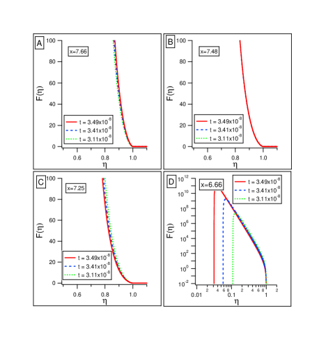
Figure 6: Application of the similarity transformation, (40), to the direct cascade at three consecutive times We take a range of values for the parameter $x$. Graph A takes $x=7.66$, graph B takes $x=7.48$, graph C takes $x=7.25$. The self-similarity of the direct cascade and the front tip is evident from graph B. For reference, graph D takes $x=6.66$, corresponding to K-Z scaling, and uses a log plot to display the entire function $F(\eta)$. It is clearly not self-similar for this value of $x$.

The behaviour of the solution of the equation for the spectrum after the singular time, ${t^{*}}$, is an interesting question. Let us consider what could be called the “bouncing back” of the spectrum from infinity after $t={t^{*}}$. Our considerations are inspired by pomeau2001 . Exactly at $t={t^{*}}$ the spectrum becomes a pure power law, $\omega^{-x_{c}}$, at large frequencies. This can be understood as follows: any finite value of $\omega$, however large, is in the wake part of the self-similar solution when $t={t^{*}}$. This wake is a pure power spectrum. Therefore at $t={t^{*}}$, we have a well defined initial condition for the evolution equation.

This spectrum is not a stationary solution (neither K-Z nor equilibrium) of the evolution equation. The subsequent evolution should follow the same principles as just before $t={t^{*}}$: the large frequency part of the spectrum has a typical timescale which goes to zero as $\omega\to\infty$. This timescale is the timescale for relaxation to a stationary K-Z spectrum with constant energy flux. Although the amplitude of this spectrum itself changes in the course of time, it does so more and more slowly after $t={t^{*}}$ so that the changes induced in the K-Z spectrum by the change of energy flux become adiabatic relative to the infinitely short timescale for the large frequency evolution. This justifies our consideration of the large time spectrum as a K-Z spectrum although it is not strictly speaking stationary in time.

Let assume now that the bouncing back of the K-Z spectrum from infinity is described by the same self-similar equation as before $t={t^{*}}$. One boundary condition is now different. The support of the self-similar spectrum now goes from zero to infinity and as $\omega\to\infty$, $n_{\omega}\sim\omega^{-x_{0}}$ with $x_{0}$ being the K-Z exponent. Near small frequencies on this stretched scale, the spectrum keeps the same power behaviour as before $t={t^{*}}$ since the timescale there is long compared to the timescale ${t^{*}}-t$ at the high frequency end. We expect that arguments which we shall present in section A are relevant here too, with the corresponding solution of the self-similar equation being unique and the free parameter required to adjust the trajectory reaching the low frequency behaviour along the stable manifold being the amplitude of the K-Z spectrum at infinity. The solution of the self-similar equation should then specify the shape of the “bend” in the spectrum seen in figure 4 and its time evolution will be then given be the same scaling of the frequencies in the similarity representation of the dynamical equations as we used before $t={t^{*}}$. Some further work will be required to make these statements more concrete.

V Derivation of the Anomalous Spectrum from the Critical Front Speed Hypothesis

In this section we present a heuristic derivation of the formula (8) promised in the introduction. The program is as follows. We first calculate the energy balance in the neighbourhood of the front tip. We will find that the condition that energy is conserved by the motion of the tip is equivalent to the condition, (45), that the solution be self similar. Next we calculate the amount of energy, $E(t_{1},t_{2})$, which enters the the frequency interval $\left[{\omega^{*}}(t_{1}),{\omega^{*}}(t_{2})\right]$ immediately behind the tip in the time interval $\left[t_{1},t_{2}\right]$. The critical front speed hypothesis is the following : the physical system selects the unique value of the front speed such that $\lim_{t_{2}\to{t^{*}}}E(t_{1},t_{2})$ is finite and nonzero for all $t_{1}<{t^{*}}$.

The basic energy balance equation for the front tip is as follows

$$\int_{t_{1}}^{t_{2}}\int_{{\omega^{*}}(t_{1})}^{{\omega^{*}}(t_{2})}\left(\frac{\partial E}{\partial t}+\frac{\partial P}{\partial\omega}\right)\ d\omega\ dt=0$$ (58)

This can be expanded to read

$$\int_{{\omega^{*}}(t_{1})}^{{\omega^{*}}(t_{2})}\left(E(\omega,t_{2})-E(\omega,t_{1})\right)\ d\omega=-\int_{t_{1}}^{t_{2}}\left(P({\omega^{*}}(t_{2}),t)-P({\omega^{*}}(t_{1}),t)\right)\ dt$$ (59)

We observe that $E(\omega,t_{1})=0$ since ${\omega^{*}}(t_{1})<\omega$ and $P({\omega^{*}}(t_{2}),t)=0$ since ${\omega^{*}}(t)<{\omega^{*}}(t_{2})$. Hence we obtain the fundamental balance equation for the front tip,

$$\int_{{\omega^{*}}(t_{1})}^{{\omega^{*}}(t_{2})}E(\omega,t_{2})\ d\omega=\int_{t_{1}}^{t_{2}}P({\omega^{*}}(t_{1}),t)\ dt.$$ (60)

Let us now calculate $P$ and $E$ near the front tip using the expansion (53) but keeping only the leading order term :

$$F(\eta)=a_{0}(1-\eta)^{3/2}+O((1-\eta)^{5/2}).$$

In terms of $\omega$ and $t$,

$$n(\omega,t)=a_{0}{\omega^{*}}(t)^{-x-3/2}({\omega^{*}}(t)-\omega)^{3/2}+O(({\omega^{*}}(t)-\omega)^{5/2}).$$

We substitute this expression for $n_{\omega}(t)$ into equations (24) and (23) and keep only the leading power of $\omega^{*}(t)-\omega$. For the energy, we obtain

$$E(\omega,t) = \Omega_{d}\ a_{0}\ \ {\omega^{*}}(t)^{-x-3/2}\ \omega^{d/\alpha}\ \left({\omega^{*}}(t)-\omega\right)^{3/2}$$ (61)

$$+O(({\omega^{*}}(t)-\omega)^{5/2}).$$

For the flux we obtain

$$P(\omega,t) = \frac{75}{8}\ a_{0}^{3}\ \omega^{3x_{0}+3}\,{\omega^{*}}(t)^{-3x-9/2}\ \left({\omega^{*}}(t)-\omega\right)^{3/2}$$ (62)

$$+O(({\omega^{*}}(t)-\omega)^{5/2}).$$

In both these expressions we can write powers of $\omega$ as $\omega^{y}=({\omega^{*}}(t)-({\omega^{*}}(t)-\omega))^{y}$ and perform a Taylor expansion in $({\omega^{*}}(t)-\omega)$. Since we are keeping only terms to leading order in $({\omega^{*}}(t)-\omega)$, we can consistently replace $\omega^{y}$ with ${\omega^{*}}(t)^{y}$ to yield the following expressions:

$$E(\omega,t) = \Omega_{d}\ a_{0}\ \ {\omega^{*}}(t)^{-x-3/2+d/\alpha}\,\left({\omega^{*}}(t)-\omega\right)^{3/2}$$ (63)

$$+O(({\omega^{*}}(t)-\omega)^{5/2}).$$

$$P(\omega,t) = \frac{75}{8}\ a_{0}^{3}\,{\omega^{*}}(t)^{3(x_{0}-x)-3/2}\,\left({\omega^{*}}(t)-\omega\right)^{3/2}$$ (64)

$$+O(({\omega^{*}}(t)-\omega)^{5/2}).$$

We now substitute these expressions into (60) and perform the integrals to leading order. Let us first consider the LHS:

$$\int_{{\omega^{*}}(t_{1})}^{{\omega^{*}}(t_{2})}E(\omega,t_{2})d\omega = \Omega_{d}\ a_{0}\int_{{\omega^{*}}(t_{1})}^{{\omega^{*}}(t_{2})}{\omega^{*}}(t_{2})^{-x-3/2+d/\alpha}\ \left({\omega^{*}}(t_{2})-\omega\right)^{3/2}d\omega+\mbox{h.o.t.}$$ (65)

$$= \frac{2}{5}\Omega_{d}{\omega^{*}}(t_{2})^{-x-3/2+d/\alpha}\left({\omega^{*}}(t_{2})-{\omega^{*}}(t_{1})\right)^{5/2}+\mbox{h.o.t.}$$

Now consider the RHS:

$$\int_{t_{1}}^{t_{2}}P({\omega^{*}}(t_{1}),t)\ dt = \frac{75}{8}\ a_{0}^{3}\ \int_{t_{1}}^{t_{2}}{\omega^{*}}(t)^{3(x_{0}-x)-3/2}\ \left({\omega^{*}}(t)-{\omega^{*}}(t_{1})\right)^{3/2}dt+\mbox{h.o.t.}$$

Let us change integration variables $t\to{\omega^{*}}(t)$:

$$= \frac{75}{8}\ a_{0}^{3}\ \int_{{\omega^{*}}(t_{1})}^{{\omega^{*}}(t_{2})}{\omega^{*}}(t)^{3(x_{0}-x)-3/2}\ \left({\omega^{*}}(t)-{\omega^{*}}(t_{1})\right)^{3/2}\left(\frac{d{\omega^{*}}}{dt}\right)^{-1}d{\omega^{*}}+\mbox{h.o.t.}$$

We now use the self-similarity condition, (45), to express the derivative in terms of ${\omega^{*}}(t)$ and perform the Taylor expansion trick again: for some power, $y$, we write : ${\omega^{*}}(t)^{y}=({\omega^{*}}(t_{1})+({\omega^{*}}(t)-{\omega^{*}}(t_{1})))^{y}={\omega^{*}}(t_{1})^{y}+\mbox{h.o.t.}$ This gives

$$= \frac{75}{8}\ a_{0}^{3}{\omega^{*}}(t_{1})^{3(x_{0}-x)-3/2}\,{\omega^{*}}(t_{1})^{-(3x_{0}-2x-d/\alpha)}\,\int_{{\omega^{*}}(t_{1})}^{{\omega^{*}}(t_{2})}\left({\omega^{*}}-\omega\right)^{3/2}d{\omega^{*}}+\mbox{h.o.t.}$$

$$= \frac{75}{8}\ a_{0}^{3}{\omega^{*}}(t_{1})^{3(x_{0}-x)-3/2}\ \left(\frac{d{\omega^{*}}}{dt_{1}}\right)^{-1}\frac{2}{5}\left({\omega^{*}}(t_{2})-{\omega^{*}}(t_{1})\right)^{5/2}+\mbox{h.o.t.}$$

Equating (65) and (LABEL:eq-int_P) and letting $t_{1}\to t_{2}$, we obtain energy balance criterion

$$\frac{d{\omega^{*}}}{dt}\ {\omega^{*}}^{2x-3x_{0}+d/\alpha}=1$$ (67)

which is equivalent to the self-similarity condition that (45) be time independent.

Now suppose we take $t_{2}-t_{1}$ to be small but finite and allow $t_{2}\to{t^{*}}$. It is clear that the energy flux, (LABEL:eq-int_P), entering the region $[{\omega^{*}}(t_{1}),{\omega^{*}}(t_{2})]$ in this last increment of time before the front reaches infinity is either infinite, a finite quantity, or zero. Our hypothesis is that the flux is finite. It certainly cannot be infinite since the entire system has finite energy. It seems unreasonable that it should be zero since the front presumably requires a supply of energy to continue moving. A finite value for the integrated flux requires that the power of $\omega(t_{2})$ in (65) is zero. This hypothesis leads to a unique value for the slope, which we shall denote by $x_{c}$. From (65):

$$\frac{2}{5}\Omega_{d}{\omega^{*}}(t_{2})^{-x-3/2+d/\alpha}\left({\omega^{*}}(t_{2})-{\omega^{*}}(t_{1})\right)^{5/2}+\mbox{h.o.t.}$$ (68)

$$= \Omega_{d}{\omega^{*}}(t_{2})^{-x-3/2+d/\alpha}\left(\frac{d{\omega^{*}}}{dt_{2}}\right)^{\frac{5}{2}}\ \frac{2}{5}(t_{2}-t_{1})^{\frac{5}{2}}+\mbox{h.o.t.}$$

$$= {\omega^{*}}(t_{2})^{-6\left(x-x_{0}-\frac{2\gamma-3\alpha}{12\alpha}\right)}\ \Omega_{d}\frac{2}{5}(t_{2}-t_{1})^{\frac{5}{2}}+\mbox{h.o.t.}.$$ (69)

In order that this remain finite but non-zero as ${\omega^{*}}(t_{2})\to\infty$, we require

$$x=x_{c}=x_{0}+\frac{2\gamma-3\alpha}{12\alpha}$$ (70)

The physical intuition behind this hypothesis is the following. If $x>x_{c}$, the front speed is slower than the critical value. The power in (69) is positive and the energy in the tip diverges as ${\omega^{*}}(t_{2})\to\infty$. The front is moving too slowly for the amount of flux flowing into it so that energy begins to pile up at the tip. On the other hand, if $x<x_{c}$, the front moves faster than the critical value. Then energy in the tip decays to zero as ${\omega^{*}}(t_{2})\to\infty$ which means that the front is moving too fast for the amount of energy supplied to it. Physically we expect that the former situation would tend to speed up the front and the latter would tend to slow it down thus providing the system with a self-regulatory mechanism which selects the marginal slope, $x_{c}$.

VI Concluding Remarks

From the work presented here, we are beginning to get a clearer understanding of how the K-Z spectrum is set up in this model and the origins of the anomalous spectrum in the wake. The most obvious and important question which we have not addressed at all here is that of whether any of this analysis is relevant for the full kinetic equation, (1). It seems unlikely that the detailed structure of the nonlinear front would carry over to the integral version of the kinetic equation. Indeed, it is difficult to see how a sharp front tip could co-exist with the k-space integrations on the RHS of (1).

Nevertheless, anomalous behaviour has been observed galtier2000 in numerical simulations of the full three-wave kinetic equation as already mentioned. This gives us reason to hope that some of the qualitative ideas contained here can be extended to more general kinetic equations. In particular, if the dynamics of the front is indeed regulated by a critical speed hypothesis of the type proposed in section V, then there is hope that an analogue can be formulated even in the absence of a sharp tip.

One might also speculate that this mechanism might occur in the evolution of the Kolmogorov spectrum of hydrodynamic turbulence since the direct cascade in this case is also of finite energy capacity. Unfortunately, in the absence of a closed kinetic equation for hydrodynamic turbulence it is not clear how one would even begin to address this question from a mathematical point of view. Nevertheless, for the purpose of stimulating debate, let us make the following conjecture. In far from equilibrium situations with stationary states which have finite capacity, the evolution towards the stationary spectrum takes place in two stages. In the first stage, $0<t<{t^{*}}$, which is rapid, the system attempts to close the connection with the dissipative sink at very high (or very low) wave-numbers. In that stage, entropy production is positive as the system attempts to explore all the available phase space subject to the constraint of energy conservation. The wake spectrum is steeper (shallower if the sink is at ${\bf k}=0$) than that of the final stationary state. This slope is determined by the requirement that a finite amount of energy per unit time is delivered to the front tip at all times less that ${t^{*}}$. After $t={t^{*}}$, energy is no longer conserved but entropy production is still positive as the system now explores a larger volume of phase space. However, the entropy production now decreases as a new front with the K-Z spectrum in its wake (between the front and ${\bf k}=\infty$) moves towards lower wave-numbers and invades the steeper spectrum set up during the first stage of evolution. While it may be difficult to confirm these conjectures in a quantitative manner for the variety of situations to which we suggest these ideas apply, it should not be too difficult to establish them (or prove them incorrect) qualitatively.

Note Added in Proof

We have subsequently analysed a second order model equation whose structure is similar to that of the differential kinetic equation studied in this paper but is analytically and numerically more tractable. We have found qualitatively similar behaviour. However the value of the anomalous exponent appears to differ from that which would be predicted by our critical front speed hypothesis.

Appendix A Analysis of the Self-similarity Equation and the Critical Front Speed

In this appendix we shall analyse the similarity equation (44) further. We wish to check that it does indeed admit solutions which reproduce the critical behaviour which we have ascribed to the solutions of its antecedent PDE in section V. Specifically, we are interested in solutions which match the $F(\eta)\sim(1-\eta)^{3/2}$ singularity at $\eta=1$ to a power law solution, $F(\eta)\sim\eta^{-x}$ as $\eta\to 0$.

Let us write (44) in the form

$$\eta^{-1+d/\alpha}\left(xF+\eta\frac{dF}{d\eta}\right)=(2(x-x_{0})-\kappa_{d})\ \frac{d^{2}}{d\eta^{2}}\left(\eta^{s}F^{4}\frac{d^{2}}{d\eta^{2}}\left(\frac{1}{F}\right)\right),$$ (71)

and look for solutions of the form $F(\eta)=A\eta^{-y}$. Substituting this form we obtain

$$(-y+x)\ \eta^{\frac{d}{\alpha}-1-y} = 3A^{2}y(y-1)(x_{0}-y)(3x_{0}-3y-1)$$ (72)

$$(2(x-x_{0})-\kappa_{d})\ \eta^{3x_{0}-3y-2}$$

We see that we can have the following solutions $y=x$ where $x$ takes one of the following values,

$$x = 0$$ (73)

$$x = 1$$ (74)

$$x = x_{0}$$ (75)

$$x = x_{0}-1/3$$ (76)

The first pair are the thermodynamic spectra, the second pair are the K-Z energy and particle spectra respectively. A fifth special value of $y$ is

$$x=x_{0}+\kappa_{d}/2.$$ (78)

What we observe from numerical solution of the O.D.E. (72), described below, is as follows. If we choose a value of $x$ which is not $x_{c}=x_{0}+\kappa_{d}/4$, then the solution, $\eta^{-x}$, makes a transition near $\eta=0$ to the state $\eta^{-y}$, where $y=x_{0}+\kappa_{d}/2$. This behaviour near $\eta=0$ balances the leading order divergences on both sides of equation (72) as $\eta\to 0$. It might be noted, although it may have no relevance to the problem under consideration, that this value for the exponent, $y$, leads to front dynamics, ${\omega^{*}}(t)=({t^{*}}-t)^{b}$ with zero $b$. This spectrum was never observed in the solutions of the P.D.E.

To find solutions of (44) which do not exhibit the $x_{0}+\kappa_{d}/2$ scaling as $\eta\to 0$, we decided to perform a set of numerical experiments. Let us write out the RHS explicitly so that we can see exactly the equation which we wish to solve:

$$\frac{1}{2(x-x_{0})-\kappa_{d}}\ \eta^{-1+\frac{d}{\alpha}} \left(xF+\eta\frac{dF}{d\eta}\right)=-\eta^{s}F^{2}\frac{d^{4}F}{d\eta^{4}}-2s\eta^{s-1}F^{2}\frac{d^{3}F}{d\eta^{3}}$$

$$+2\eta^{s}F\left(\frac{d^{2}F}{d\eta^{2}}\right)^{2}+8\eta^{s}\left(\frac{dF}{d\eta}\right)\frac{d^{2}F}{d\eta^{2}}$$

$$+4s\eta^{s-1}\left(\frac{dF}{d\eta}\right)^{3}+4s\eta^{s-1}F\frac{dF}{d\eta}\frac{d^{2}F}{d\eta^{2}}$$

$$+2s(s-1)\eta^{s-2}F\left(\frac{dF}{d\eta}\right)-s(s-1)\eta^{s-2}F^{2}\frac{d^{2}F}{d\eta^{2}}$$

The problem with integrating (A) on a computer is that for generic initial conditions, the strong power law dependences of the right hand side on the independent variable render the numerics very susceptible to round-off error and numerical instability. For example, to study the system with $\gamma=7/2$, $\alpha=1/2$, $d=1$, to which we gave a lot of consideration in section III due to its relatively large anomaly, we are required to take $3x_{0}+2=22$.

To get around this difficulty, and to aid visualisation of the global properties of the equation, we make the following change of variables :

$$F(\eta) = \eta^{a}f(\tau)$$

$$\frac{dF}{d\eta} = \eta^{a-1}g(\tau)$$ (80)

$$\frac{d^{2}F}{d\eta^{2}} = \eta^{a-2}h(\tau)$$

$$\frac{d^{3}F}{d\eta^{3}} = \eta^{a-3}k(\tau),$$

where $\tau=\log(\eta)$. By choosing

$$a=\frac{1}{2}\left(\frac{d}{\alpha}-s+3\right)=-x_{0}-\frac{\kappa_{d}}{2},$$ (81)

we can cancel all the power dependence from the system and eventually recast (A) as the the following autonomous fourth order system:

$$\frac{df}{d\tau} = g-af$$

$$\frac{dg}{d\tau} = h-(a-1)g$$

$$\frac{dh}{d\tau} = k-(a-2)h$$ (82)

$$f^{2}\frac{dk}{d\tau} = -\frac{1}{2(x-x_{0})-\kappa_{d}}\ \left(g+xf\right)-(a+2s-3)f^{2}k+2fh^{2}$$

$$+8g^{2}h+4sg^{3}+4sfgh+2s(s-1)fg^{2}-s(s-1)f^{2}h.$$

Only the region, $f\geq 0$ makes physical sense since $n_{\omega}$, and hence $F$, cannot be negative. This system is singular on the hyperplane $f=0$. This system is much easier to integrate numerically and has the added advantage that we can determine the presence of fixed points which are not obvious in the original differential equation. Let us determine these points. It is obvious that the RHS of (82) has a trivial zero at $(f,g,h,k)=(0,0,0,0)=O$ but this is clearly a singular point due to the factor of $f^{2}$ on the LHS. A second pair of nontrivial (and nonsingular) fixed points can be shown after quite a bit of algebra to exist at the points $P_{\pm}=(f_{0},af_{0},a(a-1)f_{0},a(a-1)(a-2)f_{0})$, where

$$f_{0}=\pm\left(18a(a+1)(a+(s-2)/3)(a+(s-3)/3)\right)^{-\frac{1}{2}}.$$ (83)

We are naturally only interested in the point $P_{+}$ since $P_{-}$ lies in the negative $f$ region. The factors $(a+(s-2)/3)$ and $(a+(s-3)/3)$ are interesting for the following reason. If we substitute back in $s=3x_{0}+2$ and the value of $a$ from (81), these two factors are simply $-\kappa_{d}/2$ and $-\kappa_{i}/2$ respectively. At the transition points between finite and infinite capacity the fixed point runs away to infinity which suggests that it has a central role to play in organising the critical solution in the finite capacity case.

Let us now look for a numerical solution of this system which mirrors the solutions of the differential kinetic equation. All the simulations in this section were done using the transformed system, (82), for which a standard out-of-the-box adaptive Runge-Kutta routine seemed to work fine. Suppose we want a solution for the wake of the form $F(\eta)\sim\eta^{-x}$ as $\eta\to 0$. In the new variables this is equivalent to demanding

$$f(\eta) \sim A\eta^{-a-x}$$

$$g(\eta) \sim -xf(\eta)$$

$$h(\eta) \sim x(x+1)f(\eta)$$

$$k(\eta) \sim -x(x+1)(x+2)f(\eta)$$

as $\eta\to 0$ or as $\tau\to\-\infty$. If $x<-a=x_{0}+\kappa_{d}/2$, which is the case, then we observe that the wake is described by a trajectory for which $(f,g,h,k)\to(0,0,0,0)$ as $\tau\to-\infty$. The wake is the singular point, $O$, of the system, (82). As we approach $\eta\to 1$ we must reproduce the front structure described in section IV. Thus we require a trajectory for which $(f,g,h,k)\to F$ as $\tau\to 0$, where $F=(0,0,\infty,\infty)$. We require a trajectory which links these two singular points.

In our numerical simulations we rescaled the variables as follows,

$$f \to \frac{f}{f_{0}}$$

$$g \to \frac{g}{af_{0}}$$

$$h \to \frac{h}{a(a-1)f_{0}}$$

$$k \to \frac{k}{a(a-1)(a-2)f_{0}}$$

This maps the point $P_{+}\to(1,1,1,1)$ for ease of visualisation. The only difference is that since $a<0$, the signs of $g$ and $k$ are swapped so that the wake part of the solution must now approach $O$ from the direction $(0^{+},0^{+},0^{+},0^{+})$ and the front tip, $F$, is now at $(0^{+},0^{+},\infty,-\infty)$.

It turns out to be difficult to find a trajectory linking $F\to O$. We performed a series of experiments integrating backwards from $1-\eta=\varepsilon$, with $\varepsilon<<1$, towards $\eta=0$. Because we cannot specify initial data exactly at the singular point, $F$, we were required to manually tune the initial conditions quite a bit in order to to reproduce the $F(\eta)\sim(1-\eta)^{3/2}$ structure near the tip. The remaining adjustable parameter is the equation is $x$. We again choose to study the case $\gamma=7/2$, $\alpha=1/2$, $d=1$. Two generic types of trajectory emerge as we vary $x$. We visualise these trajectories in 4 dimensional phase space as a pair of projections of the actual trajectory onto the $(f,g)$ and $(h,k)$ planes respectively, hence the apparent intersections.

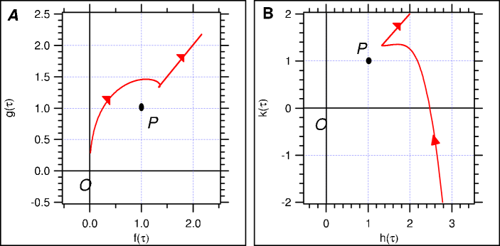
Figure 7: Trajectory in $(f,g,h,k)$ space for $x=7.56275$, which is less than the critical value.

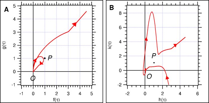
Figure 8: Trajectory in $(f,g,h,k)$ space for $x=7.56975$, which is greater than the critical value.

Figure 9: Trajectory in $(f,g,h,k)$ space for $x=7.56875\approx x_{c}$. Since it is impossible to specify the data exactly, if we integrate for long enough in $\tau$ this trajectory eventually deflects away from $O$.

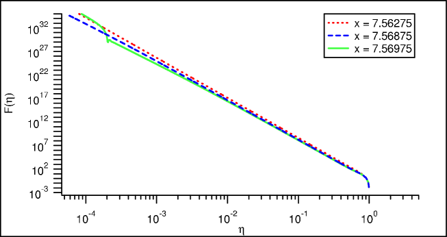
Figure 10: Plots of the $F(\eta)$ associated with the trajectories in figures 7, 8 and 9 after converting from the $(f,g,h,k)$ and $\tau$ variables back to $F$ and $\eta$ variables. The scales are log-log.

Figure 7 shows what happens when $x$ is slightly less than $x_{c}$. The trajectory leaves the front tip and heads towards the fixed point, $P$, but deflects to the right and is quickly attracted onto the line corresponding to $F(\eta)\sim\eta^{-x_{0}-\kappa_{d}/2}$. Figure 8 shows the corresponding trajectory when $x$ is slightly greater than $x_{c}$. This time the trajectory deflects to the left as it approaches the fixed point, $P$, and is attracted towards the singular point, $O$. Before it reaches there however, it is deflected and is rapidly attracted back onto the $F(\eta)\sim\eta^{-x_{0}-\kappa_{d}/2}$ solution again. The transition point between these two trajectories is illustrated in figure 9. Further analysis is required to determine the exact nature of the critical trajectory. It is not clear whether it will eventually deflect away from $O$ for sufficiently small $\eta$. Of course, in practical terms there is a limit placed on the extent of the scaling region by the left boundary of the inertial range which cannot extend all the way to 0 in a real experiment.

The system is very sensitive to the value of $x$. The values of $x$ for the trajectories shown differ only in the fourth decimal place. In figure 10, the form of the function $F(\eta)$ is shown for the three cases discussed above, after transforming back from the $(f,g,h,k)$, $\tau$ variables. The integration was again done for the case $\gamma=7/2$, $\alpha=1/2$, $d=1$. Despite the small difference in the values of $x$ in the equation the difference in asymptotic slopes is $7.56$ for the critical slope versus $8.5$ for the other two.

Appendix B Outline of Numerical Methods

In order to study how the K-Z spectrum is set up from some given initial condition we wrote some code to solve (13) numerically. In this appendix we briefly outline the approach used. Write equation (13) in the form

$$\frac{\partial n_{\omega}}{\partial t}=f\left[n_{\omega}\right]\frac{\partial^{4}n_{\omega}}{\partial\omega^{4}}+g\left[n_{\omega}\right]\frac{\partial^{3}n_{\omega}}{\partial\omega^{3}}+h\left[n_{\omega}\right]+F\left[n_{\omega}\right]-\nu\left[n_{\omega}\right],$$ (84)

where

$$f\left[n_{\omega}\right] = -\Lambda^{-1}_{\omega}\omega^{s}n^{2}$$ (85)

$$g\left[n_{\omega}\right] = -2\Lambda^{-1}_{\omega}s\omega^{s-1}n^{2}$$ (86)

$$h\left[n_{\omega}\right] = \Lambda^{-1}_{\omega}\left\{\omega^{s}\left(2n\left(\frac{\partial^{2}n}{\partial\omega^{2}}\right)^{2}+8\left(\frac{\partial n}{\partial\omega}\right)^{2}\frac{\partial^{2}n}{\partial\omega^{2}}\right)\right.$$ (87)

$$\hskip 28.45274pt+2s\omega^{s-1}\left(2\left(\frac{\partial n}{\partial\omega}\right)^{3}+2n\frac{\partial n}{\partial\omega}\frac{\partial^{2}n}{\partial\omega^{2}}\right)$$

$$\hskip 28.45274pt+s(s-1)\omega^{s-2}\left.\left(2n\left(\frac{\partial n}{\partial\omega}\right)^{2}-n^{2}\frac{\partial^{2}n}{\partial\omega^{2}}\right)\right\}$$

$$\Lambda_{\omega} = \frac{\Omega_{\bf k}}{\alpha}\omega^{\frac{d}{\alpha}-1}$$ (88)

$$s = 3x_{0}+2.$$ (89)

We are now including forcing and damping terms, $F\left[n_{\omega}\right]$ and $\nu\left[n_{\omega}\right]$ which can be chosen as appropriate. We performed the following implicit time discretisation,

$$\frac{n_{\omega}(t+\Delta t)-n_{\omega}(t)}{\Delta t} = f\left[n_{\omega}(t)\right]\frac{\partial^{4}n_{\omega}(t+\Delta t)}{\partial\omega^{4}}+g\left[n_{\omega}(t)\right]\frac{\partial^{3}n_{\omega}(t+\Delta t)}{\partial\omega^{3}}$$ (90)

$$+h\left[n_{\omega}(t)\right]+F\left[n_{\omega}(t+\Delta t)\right]-\nu\left[n_{\omega}(t+\Delta t)\right],$$

with the aim of enhancing the stability of the higher order derivatives. This can be rearranged to yield a time stepping algorithm in the form

$$n_{\omega}(t+\Delta t)=L^{-1}\left[n_{\omega}(t)\right]B\left[n_{\omega}(t)\right],$$ (91)

where

$$L\left[n_{\omega}\right] = 1+\Delta t\ f\left[n_{\omega}\right]\frac{\partial^{4}}{\partial\omega^{4}}+\Delta t\ g\left[n_{\omega}\right]\frac{\partial^{3}}{\partial\omega^{3}}$$ (92)

$$B\left[n_{\omega}\right] = n_{\omega}+\Delta t\ h\left[n_{\omega}\right]+\Delta t\ F\left[n_{\omega}\right].$$ (93)

The time evolution operator, $L\left[n_{\omega}\right]$, and source, $B\left[n_{\omega}\right]$, are approximated using centred difference representations for the derivatives and a standard linear solver used to perform the inversion at each time-step. Implementing consistent boundary conditions is a tricky task. For all of the simulations presented here, the equation was solved from a compactly supported initial condition either in a frequency interval sufficiently large that the solution does not reach the boundary within the time allotted or with the damping chosen sufficiently strong to prevent the solution from ever reaching the boundary.

Most of the simulations presented here are of a freely decaying initial energy distribution so $F[n_{\omega}]=0$. The damping was chosen to be zero over most of the interval but increasing strongly for $\omega<\omega_{L}$ and $\omega>\omega_{R}$ to produce regions of strong dissipation at large and small scales. We typically used approximately $10$ grid points per unit frequency interval in our discretisation. The simulations presented here used up to 20000 grid-points. The number of grid points is practically limited by the fact that one must recompute and invert the time evolution operator, (92), at each time-step. Lacking any reliable stability criteria for the nonlinear discretisation scheme described above, the choice of time-step was essentially made by trial and error. Once a time-step was found for which the evolution seemed stable, we ran with it. We were aided in choosing this time-step by monitoring the two conservation laws associated with the total energy and total particle number. Typically, and unsurprisingly, the numerics become unstable most easily at the front tip. This instability is worse for steeper spectra when the front travels faster. The necessity of reducing the time-step to resolve this structure as the tip increases in speed also put practical limits on the time interval we could simulate for. Retrospectively, we would like to do the numerics using an adaptive grid which tracks the front. Such a method would probably yield great increases in efficiency and stability. Unfortunately at the outset, we did not really appreciate that the code would be required to tackle this problem. We settled for validating our computations by checking that our final results remained unchanged when the time-step was reduced by a factor of two.

References

- [1] Lacey A.A., Ockendon J.R., and Tayler A.B. Waiting time solutions of a nonlinear diffusion equation. SIAM J. Appl. Math., 42(6):1252–1264, 1982.
- [2] P.J. Aucoin and A.C. Newell. Semidispersive wave systems. Jour. Fluid Mech., 49:593–609, 1971.
- [3] D.J. Benney and A.C. Newell. Sequential time closures of interacting random waves. Journal of Mathematics and Physics, 46:363, 1967.
- [4] S. Dyachenko, A.C. Newell, A. Pushkarev, and V.E. Zakharov. Optical turbulence: Weak turbulence, condensates and collapsing filaments in the Nonlinear Schrodinger equation. Physica D, 57:96–160, 1992.
- [5] G.E. Falkovich and A.V. Shafarenko. Non-stationary wave turbulence. J. Nonlinear Sci., 1:452–480, 1991.
- [6] S. Galtier, S.V. Nazarenko, A.C Newell, and A. Pouquet. A weak turbulence theory for incompressible MHD. J. Plasma Phys., 63:447–488, 2000.
- [7] K. Hasselmann. On the nonlinear energy transfer in a gravity wave spectrum I. J. Fluid Mech., 12:481–500, 1962.
- [8] K. Hasselmann. On the nonlinear energy transfer in a gravity wave spectrum II. J. Fluid Mech., 15:273–281, 1963.
- [9] R. Lacaze, P. Lallemand, Y. Pomeau, and S. Rica. Dynamical formation of a Bose-Einstein condensate. Physica D, 152-153:779–786, 2001.
- [10] A.C. Newell and P.J. Aucoin. Semidispersive wave systems. J. Fluid. Mech., 49:593–609, 1971.
- [11] A.C. Newell, S. Nazarenko, and L. Biven. Wave turbulence and intermittency. Physica D, 152-153:520–550, 2001.
- [12] C.S. Ng and A. Bhattachargee. Interaction of shear alfven wave packets : Implication for weak magnetohydrodynamic turbulence in astrophysical plasmas. Astrophysical Journal, 465(2 part 1):845–854, 1996.
- [13] V.E. Zakharov and N. Filonenko. The energy spectrum for stochastic oscillation of the fluid surface. Doklady Akad. Nauk SSSR, 170:1292–1295, 1966.
- [14] V.E. Zakharov and R.Z. Sagdeev. On spectra of acoustic turbulence. Dokl. Akad. Nauk SSSR, 192(2):297–299, 1970. English transl., Soviet Phys. JETP 35 (1972), 310-314.
- [15] V.S. Zakharov, V.S. Lvov, and G. Falkovich. Kolmogorov Spectra of Turbulence. Springer-Verlag, Berlin, 1992.
- [16] Y.B. Zel’dovich and A.S. Kompaneets. On the theory of heat propogation for temperature dependent thermal conductivity. In Collection Commemorating the 70th Anniv. of A.F. Joffe. Izdat. Akad. Nauk SSSR, Moscow, 1950.