Microcanonical Thermodynamic Properties of Helium Nanodroplets

Abstract

The density of states and other thermodynamic functions of helium nanodroplets are calculated for a microcanonical ensemble with both energy and total angular momentum treated as conserved quantum numbers. These functions allow angular momentum conserving evaporative cooling simulations. As part of this project, a recursion relationship is derived for the reduction to irreducible representations of the n’th symmetric power of the irreducible representations of the rotation group. These give the distribution of total angular momentum states generated by putting multiple quanta into a ripplon or phonon mode of the droplet, each of which is characterized by a angular momentum quantum number.

I Introduction

Spectroscopy of atoms and molecules dissolved in superfluid helium nanodroplets has become a field of intense activity. Such nanodroplets rapidly cool by evaporation, reaching final temperatures of $\approx 0.37$ K Hartmann95 . There is a long history of their formation and study by mass spectroscopic methods Becker61 ; Northby01 . Vibrational Goyal92 ; Hartmann95 ; Callegari01 , electronic Stienkemeier95 ; Hartmann96a ; Stienkemeier01 , and rotational Reinhard99 ; Callegari00c ; Grebenev00a transitions have been observed. Part of the interest in this field is that helium droplets provide a nearly ideal matrix Lehmann98 for isolation of highly unstable compounds. Many novel compounds and clusters have been synthesized and spectroscopically studied in this unique environment Goyal93 ; Hartmann96 ; Higgins96 ; Nauta99b ; Nauta01c .

There have been several previously reported calculations of the evaporative cooling of helium nanodroplets Gspann82 ; Brink90 , and these have predicted a terminal temperature in excellent agreement with that later observed experimentally Hartmann95 . These calculations, however, have not considered angular momentum conservation, which obviously imposes constraints on droplet cooling in a high vacuum environment. In order to address the question of the possible trapping of angular momentum in a cooling droplet, we have undertaken a new study of the evaporative cooling of the nanodroplets, but including angular momentum conservation, using methods analogous to “Phase Space Theory” calculations of unimolecular dissociation Baer96 . Necessary inputs to such calculations are the density of states and integrated density of states of helium nanodroplets, over the energy and angular momentum range sampled in the evaporative cooling trajectories of nanodroplets.

The angular momentum resolved density of states of helium nanodroplets is not available in the literature. While the calculation of this quantity is largely based upon straightforward extensions of standard convolution methods, there is one particular point that was not. The distribution of angular momentum states produced by excitation of an arbitrary number of quanta in a $(2L+1)$ degenerate vibrational state of angular momentum quantum number $L$ was required. This distribution is provided by the reduction of the $n$’th symmetric product of the $L$’th irreducible representation of the group of transformations of a sphere, $K$. While the equivalent reduction for common molecular point groups is well known Wilson55 , the present author could not locate the general result for $K$, and has derived a recursion relationship that provides the needed reduction. This is presented in the present paper, along with a derived asymptotic expression, which is of the same form as the thermal distribution of a rigid spherical top.

The density of both ripplon and phonon modes are considered separately. In each case, the simple scaling of the excitation spectrum with droplet size (and thus number of helium atoms), allows the density of states to be derived as a unique function of a reduced energy. These functions have been fit to simple analytical expressions which provide excellent approximations over the range of energy and angular momentum of interest. In particular, it is found that the distribution of angular momentum quantum states is of the form of the thermal distribution of rotation for a rigid spherical top, with a reduced energy dependent effective inverse “temperature” that changes slowly with energy.

II Ripplon Excitations

The lowest energy excitations of a pure droplet are ripplons, which are quantized capillary waves on the surface of the droplets. The properties of such waves on spherical drops are thoroughly described in the classic text on hydrodynamics by Lamb Lamb . Classically, each ripplon mode involves a modulation of the surface of the droplet, with

$$r(\theta,\phi)=r_{0}+\sum_{L,M}Re\left(A_{LM}Y_{LM}(\theta,\varphi)e^{i\omega_{L}t}\right)$$ (1)

where $L\geq 2$ and

$$\omega_{L}=\sqrt{L(L-1)(L+2)}\,\omega_{0}$$ (2)

$$\omega_{0}=\sqrt{\frac{\sigma}{m\rho R^{3}}}=\sqrt{\frac{4\pi\sigma}{3mN}}$$ (3)

and $\sigma$ is the helium surface tension (approximated by the bulk zero temperature value of 0.363 mJ/m²), $m$ is the atomic mass of helium, $\rho$ is the number density of helium (approximated by the bulk zero temperature value of 0.0218 Å^-3), and $R=\sqrt[3]{\frac{3N}{4\pi\rho}}=2.22N^{1/3}$ Å with $N$ equal to the number of helium atoms in the droplet. Given that the spectrum of ripplon modes is proportional to a common factor that contains the size dependence, the thermodynamic functions of the ripplon modes are universal functions of a reduced energy which has unit value equal to $E_{\textrm{r}}=\hbar\omega_{0}=3.77/\sqrt{N}\,k_{\textrm{\scriptsize{B}}}$K.

The integrated total state count, $N_{E}$, and the total density of states, $\rho_{E}$, can be calculated from the spectrum of ripplon mode frequencies using the Beyer-Swinehart direct count method Baer96 . In addition to the spectrum, one needs the degeneracy of a state with $n_{L}$ quanta in the ripplon mode with quantum number L. This is equal to the number of distinct ways of putting $n_{L}$ identical objects into $2L+1$ bins and is equal to $g(n_{L},L)=\frac{(n_{L}+2L)!}{(2L)!n_{L}!}$ Reif65 . Define $N_{E}(E,L)$ to be the integrated density of states calculated using only ripplon modes with angular momentum quantum numbers less than or equal to $L$. We can recursively calculate the total integrated density of states by using:

$$N_{E}(E,L=2) = \sum_{n_{2}}\Phi(E-\hbar\omega_{2}n_{2})g(n_{2},2)$$ (4)

$$N_{E}(E,L) = \sum_{n_{L}}N(E-\hbar\omega_{L}n_{L},L-1)g(n_{L},L)$$ (5)

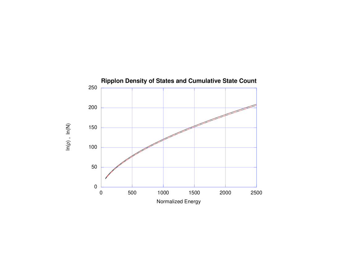
Figure 1: Plot of the natural log of the integrated density of states and density of states in reduced energy units. The integrated density is slightly higher than the density of states.

where the unit step function is defined by $\Phi(x)=1(0)$ for x greater or equal to (or less than) zero. In the Beyer-Swinehart algorithm, the above are calculated using an energy bin size, $\delta E$ sufficiently small that each $\omega_{L}/\delta E$ can be approximated by an integer. A step size of $0.1$ reduced energy unit was used in this work. The calculated values of $N_{E}$ and $\rho_{E}$ are plotted on figure 1. We have fitted the calculated integrated density of states to the expression

$$N_{E}=\exp\left(aE^{4/7}+bE^{1/7}\right)$$ (6)

Values of a = 2.5118 and b= -3.4098 minimized the root mean squared fractional errors over the interval $E=50--2500$. Changing the step size in the calculation and refitting the integrated density of states gave values of a = 2.5118 and b = -3.4110. The leading power of $4/7$ can be derived by equating the high temperature limit of the microcanonical and canonical ensemble values of energy and entropy (which is proportional to $\ln(\rho_{E})$ in the microcanonical case). The power of $1/7$ for the correction term was selected based upon the slope, on a log-log plot, of $N_{E}E^{-4/7}$ vs. $E$. The expression for $N_{E}$ given in Eq. 6 agrees with the Beyer-Swinehart direct count to within $\pm 5$% while $N_{E}$ increases by more than 83 order of magnitude over the reduced energy range $50-2500$. Using standard expressions McQuarrieText for the thermodynamic functions of a microcanonical ensemble, we can derive the following:

$$\rho_{E}(E) = \left(\frac{{\textrm{d}}N_{E}}{{\textrm{d}}E}\right)=N_{E}(E)\left[\frac{4}{7}aE^{-3/7}+\frac{1}{7}bE^{-6/7}\right]$$ (7)

$$S_{E}(E) = k_{\textrm{\scriptsize{B}}}\ln(\rho_{E}(E))=k_{\textrm{\scriptsize{B}}}\left[aE^{4/7}+bE^{1/7}+\ln\left(\frac{4}{7}aE^{-3/7}+\frac{1}{7}bE^{-6/7}\right)\right]\stackrel{{\scriptstyle E\gg 1}}{{\rightarrow}}k_{\textrm{\scriptsize{B}}}aE^{4/7}$$ (8)

$$T_{E}(E) = \left(\frac{{\textrm{d}}S}{{\textrm{d}}E}\right)^{-1}=\frac{1}{k_{\textrm{\scriptsize{B}}}}\frac{28aE^{10/7}+7E}{16a^{2}E+8abE^{4/7}-12aE^{3/7}+b^{2}E^{1/7}-6b}\stackrel{{\scriptstyle E\gg 1}}{{\rightarrow}}\frac{1}{k_{\textrm{\scriptsize{B}}}}\frac{7}{4a}E^{3/7}$$ (9)

$$C_{V} = \left(\frac{{\textrm{d}}T}{{\textrm{d}}E}\right)^{-1}=$$

$$\frac{k_{\textrm{\scriptsize{B}}}\left(16a^{2}E+8abE^{4/7}-12aE^{2/7}-6b\right)^{2}}{6\left(32a^{3}E^{10/7}+32a^{2}bE-56a^{2}E^{6/7}+10ab^{2}E^{4/7}-48abE^{3/7}+b^{3}E^{1/7}-7b^{2}\right)}$$

$$\stackrel{{\scriptstyle E\gg 1}}{{\rightarrow}}k_{\textrm{\scriptsize{B}}}\frac{a}{4}E^{4/7}$$

$S_{E}$, $T_{E}$, and $C_{V}$ are the microcannonical values of the entropy, temperature, and heat capacity due to the droplet modes as a function of reduced rippon energy. The density of states, $\rho_{E}$, can be compared with $0.311E^{-5/7}\exp(2.49E^{4/7})$ derived by Brink and Stringari Brink90 through inverse Laplace Transformation of the high temperature canonical partition function using the stationary phase approximation. (Their reported results have been converted to the normalized roton energy units used in this work). It can be seen that the exponential dependence of the density of states is almost identical, but there is a slight difference in the power of the energy dependence of the exponential prefactor.

For isolated helium nanodroplets, angular momentum as well as energy is a conserved quantity, and thus the proper statistical ensemble is one that sums only over states of the same energy and total angular momentum. As a first step in the calculation of the properties of this ensemble, we have derived a regression expression that determines $N_{J}(J,n_{L},L)$ which is the number of states of total angular momentum quantum number $J$ that are generated from placing $n_{L}$ quanta in a ripplon mode with angular momentum $L$. We “count” such that each “state” is an irreducible representation with $2J+1$ values of the projection quantum number. This recursion expression and its derivation is given in the Appendix to this paper.

The individual values of $N_{J}(J,n_{L},L)$ are quite irregular and do not appear to derive from any simple expression. However, the sum of states, of course, gives the simple expression:

$$\sum_{J}(2J+1)N_{J}(J,n_{L},L)=g(n_{L},L)=\frac{(n+2L)!}{(2L)!n_{L}!}$$ (11)

Also, the mean value of the squared angular momentum has been empirically found to be given by a simple expression:

$$<J(J+1)>_{n_{L},L}=n_{L}\left[L(L+1)+\frac{1}{2}L(n_{L}-1)\right]$$ (12)

If we ignored the Bose symmetry (i.e. treated the angular momenta of different quanta in the same Ripplon mode as uncorrelated), we would not have the last term on the right hand side. The Bose symmetry increases the mean squared angular momentum because ripplon excitations have a greater probability of being in the same direction than if they where distinguishable. This closed form expression can be used to sum a thermal distribution of ripplons as a function of inverse temperature in reduced energy units, $\beta=E_{\textrm{r}}/k_{\textrm{\scriptsize{B}}}T$.

$$<J(J+1)> = \sum_{n_{L},L}<J(J+1)>_{n_{L},L}g(n_{L},L)\exp\left(-\beta n_{L}\sqrt{L(L-1)(L+2)}\right)$$ (13)

$$= \sum_{L}L(L+1)\left[\frac{2L+1}{e^{\beta\sqrt{L(L-1)(L+2)}}-1}\right]\left[1+\frac{1}{2L\left(e^{\beta\sqrt{L(L-1)(L+2)}}-1\right)}\right]$$

If we neglect the correlations induced by the Bose symmetry of the ripplon modes, we get the same result as above but with the last term on the right hand side omitted.

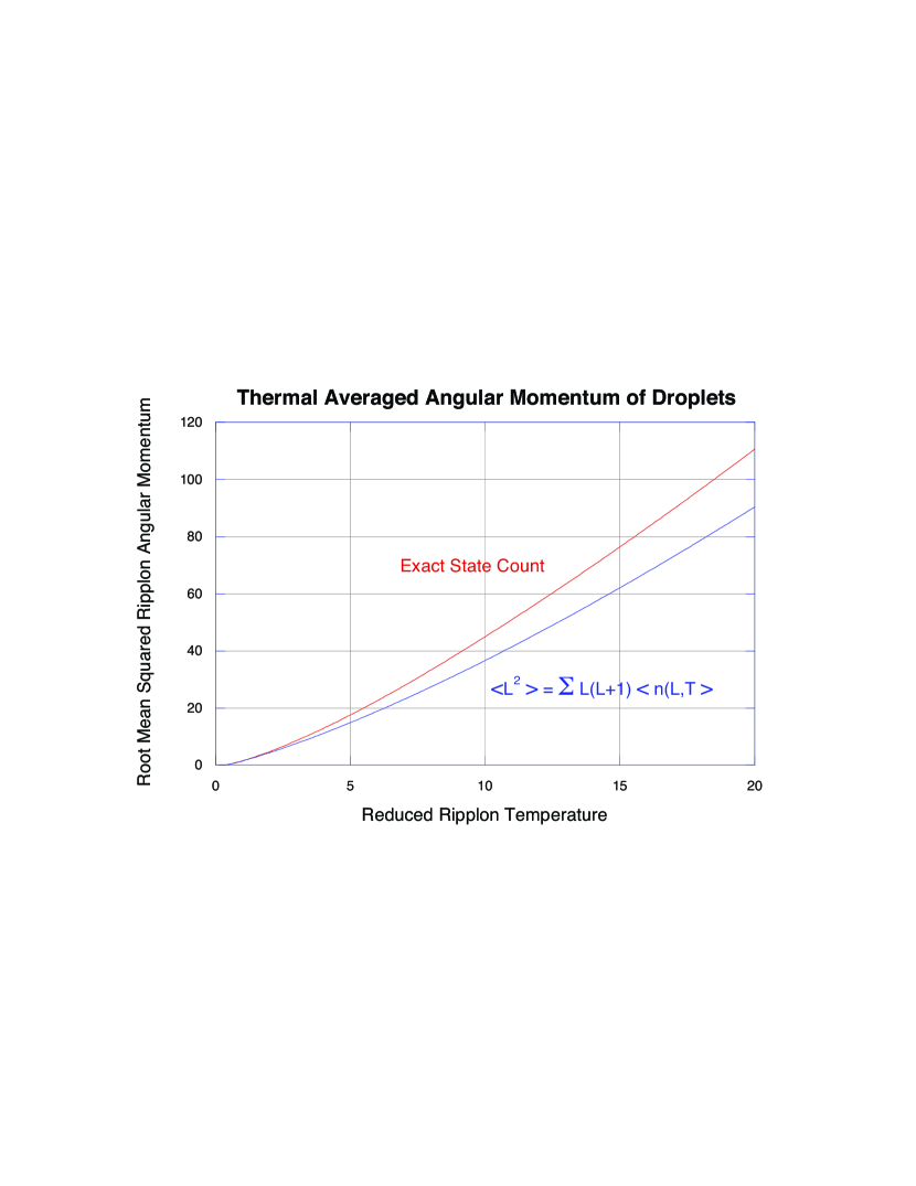
Figure 2: Plot of the Root Mean Squared total thermal angular momentum in ripplons as a function of reduced temperature. It can bee seen that the effect of the Bose correlations of the ripplon excitations increases the mean angular momentum by about 20% over the uncorrelated result.

In a previous paper,the present author used the uncorrelated expression to calculate the root mean squared averaged angular ripplon angular momentum as a function of droplet size Lehmann99b . Figure 2 shows a plot of the thermally averaged value of ${\bf J}^{2}$ calculated both neglecting the Bose symmetry and by explicit thermal average over the present Microcanonical results. It is seen that the exact calculation is modestly higher than for the uncorrelated prediction, but by a nearly constant factor of approximately 20%.

Given $N_{J}(J,n_{L},L)$, the $J$ restricted state count and density of states can be computed using a modification of the Beyer-Swinehart direct count. Define $N_{EJ}(E,J,L)$ to the integrated density of states with total angular momentum $J$, but including excitation only in ripplon modes up to angular momentum quantum number $L$. The following recursion relation is easily derived by using the triangle rule:

$$N_{EJ}(E,J,L=2) = \sum_{n_{2}}\Phi(E-\hbar\omega_{2}n_{2})N_{J}(J,n_{2},2)$$ (14)

$$N_{EJ}(E,J,L) = \sum_{n_{L},J^{\prime}}\sum_{J^{\prime\prime}=|J-J^{\prime}|}^{J+J^{\prime}}N_{EJ}(E-\hbar\omega_{L}n_{L},J^{\prime\prime},L-1)N_{J}(J^{\prime},n_{J},L)$$ (15)

for each $E$, we need to iterate on $L$ until $\hbar\omega_{L}>E$ to get the complete integrated density of states, $N_{EJ}(E,J)$, with total angular momentum $J$. We have explicitly calculated $N_{EJ}(E)$ for $E\leq 200.$ by this procedure. It was found that for each $E>50$, $N_{EJ}(E,J)$ has a distribution that accurately fits the functional form:

$$N_{EL}(E,J)=N_{E}(E)(2J+1)\sqrt{\frac{\beta_{L}(E)^{3}}{\pi}}\exp\left(-\beta_{L}(E)(J+1/2)^{2}\right)$$ (16)

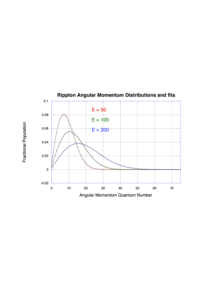
Figure 3: Plot of normalized integrated density of states as function of total angular momentum quantum number for three different values of the reduced energy. Also plotted are the distributions predicted by fits of these distributions to a thermal distribution of a spherical top, as given by Eq. 16.

which is the form of the thermal distribution for a spherical rigid rotor. Figure 3 shows plots of the calculated distributions compared to the fitted “thermal” form for several values of the reduced energy.

Assuming this “thermal” distribution of states with different rotational quantum numbers, The value of $\beta_{L}(E)$ can be calculated if we know the mean value of total angular momentum, $<J(J+1)>$, over all states up to a given energy by using $<J(J+1)>=\frac{3}{2}\beta_{L}^{-1}$. Using the relationship given in Eq. 12, we have derived a recursion relationship to calculate this quantity without having to explicitly enumerate all the states as a function of $J$. Let $A(E)$ be the average of the total angular momentum quantum numbers for all states up to reduced energy $E$, and $A(E,L)$ the same quantity, but calculated only using ripplon modes with quantum numbers up to $L$. Since angular momentum in different modes are uncorrelated, the total angular momentum is just the sum of angular momentum in each individual mode. It is straightforward to derive that

$$N_{E}(E,L)A(E,L) = \sum_{n_{L}}g(n_{L},L)N_{E}(E-\hbar\omega_{L}n_{L},L-1)\times$$ (17)

$$\left(A(E-\hbar\omega_{L}n_{L},L-1)+n_{L}\left[L(L+1)+\frac{1}{2}L(n_{L}-1)\right]\right)$$

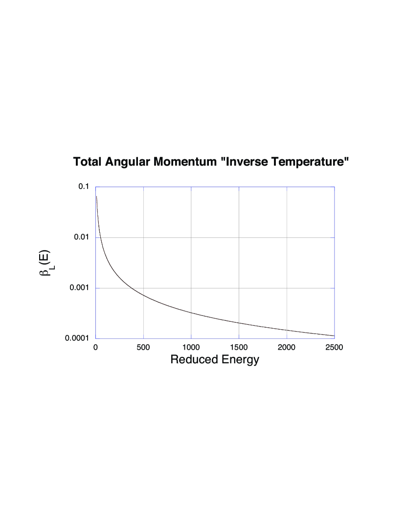
Figure 4: Plot of $\beta_{L}(E)$ as function of reduced energy. The values of $\beta_{L}$ where calculated both by from the mean value of the squared total angular momentum, as calculated by the recursion relations, and using Eq. 18. These two values agree to better than the resolution of the plot.

The inverse “rotational temperature”, $\beta_{L}(E)$, can be calculated by using the standard spherical top relation $A(E)=3/(2\beta_{L}(E))$. Using this procedure, $\beta_{L}(E)$ has been calculated for $E=10-2500.$. The values of $\beta_{L}(E)$ are plotted in figure 4 along with a fit through the points to a power law in energy:

$$\beta_{L}(E)=cE^{-8/7}+dE^{-13/7}$$ (18)

with $c=0.8680$ and $d=0.9639$. A fit the the values calculated using an energy bin of 0.01 reduced units gave $c=0.8679$ and $0.9759$. The $\beta_{L}$ values from this fit are also displayed on figure 4, but cannot be distinguished on the scale of the plot. The $\beta_{L}(E)$ calculated with Eq. 18 agrees with the calculated values to within 0.1% for $E=100-2500$ and to within 1% for $E=50-100$. The reduction in accuracy in this domain is because the calculated values of $\beta_{L}(E)$ oscillate around the value predicted by Eq. 18. The leading power of -8/7 in $\beta_{L}(E)$ can be derived by equating the high temperature limit for the mean value of the total angular momentum squared for the canonical and microcanonical ensemble.

Using the standard relationships, we can use calculate the thermodynamic quantities as a function of reduced ripplon energy and total angular momentum of the droplet as:

$$\rho_{EJ}(E,J) = \left(\frac{\partial N_{E}}{\partial E}\right)_{J}=N_{EJ}\left[\frac{4}{7}aE^{-3/7}+\frac{1}{7}bE^{-6/7}+\left(\frac{3}{2\beta_{L}}-\left(J+\frac{1}{2}\right)^{2}\right)\left(\frac{d\beta_{L}}{dE}\right)\right]$$ (19)

$$S_{EJ}(E,J) = k_{b}\ln\left(\rho_{EJ}\right)=k_{b}\left[aE^{4/7}+bE^{1/7}+\ln(2J+1)+\frac{1}{2}\ln\left(\frac{\beta_{L}^{3}}{\pi}\right)-\beta_{L}\left(J+\frac{1}{2}\right)^{2}\right.$$ (20)

$$\left.+\ln\left[\frac{4}{7}aE^{-3/7}+\frac{1}{7}bE^{-6/7}+\left(\frac{3}{2\beta_{L}}-\left(J+\frac{1}{2}\right)^{2}\right)\left(\frac{d\beta_{L}}{dE}\right)\right]\right]$$

$$\frac{1}{k_{b}T_{EJ}(E,J)} = \frac{1}{k_{b}}\left(\frac{\partial S_{SJ}}{\partial E}\right)_{J}=\frac{4}{7}aE^{-3/7}+\frac{1}{7}bE^{-6/7}+\left(\frac{3}{2\beta_{L}}-\left(J+\frac{1}{2}\right)^{2}\right)\left(\frac{d\beta_{L}}{dE}\right)$$ (21)

$$+\frac{-\frac{12}{49}aE^{-10/7}-\frac{6}{49}bE^{-13/7}+\left(\frac{3}{2\beta_{L}}-\left(J+\frac{1}{2}\right)^{2}\right)\left(\frac{d^{2}\beta_{L}}{dE^{2}}\right)-\frac{3}{2\beta_{L}^{2}}\left(\frac{d\beta_{L}}{dE}\right)^{2}}{\left[\frac{4}{7}aE^{-3/7}+\frac{1}{7}bE^{-6/7}+\left(\frac{3}{2\beta_{L}}-\left(J+\frac{1}{2}\right)^{2}\right)\left(\frac{d\beta_{L}}{dE}\right)\right]}$$

If we neglect $\frac{3}{2\beta_{L}^{2}}\left(\frac{d\beta_{L}}{dE}\right)^{2}$ in Eq. 21 (which $\approx 3.2E^{-4/7}$ times $\frac{12}{49}aE^{-10/7}$ that it is added to), then the equation for $T_{EJ}$ can be shown to reduce in the high energy limit to:

$$T_{EJ}(E,J)=T_{E}(E)+0.48E^{-9/7}\left(\frac{3}{2\beta_{L}}-\left(J+\frac{1}{2}\right)^{2}\right)+O\left(\frac{3}{2\beta_{L}}-\left(J+\frac{1}{2}\right)^{2}\right)^{2}$$ (22)

$T_{EJ}$ decreases monotonically with $J$ for fixed $E$. $T_{EJ}(E,0)=T_{E}(E)+0.83E^{-1/7}$, while for the RMS value of $J$, $T_{EJ}(E,J)=T_{E}(E)$. However, for $J\gg 1.2E^{6/7}$, $T_{EJ}\rightarrow 1.01E^{15/7}J^{-2}$, values much below $T_{E}(E)$ for the same value of $E$.

III Phonon Excitations

Starting at higher energy than the surface ripplon modes are phonon (compressional) excitations of the helium droplets. These normal modes are characterized by two quantum numbers, $n,L$, where $n=1,2,\dots$ is the number of radial nodes and $L$ is the angular momentum quantum number. Each normal node can be characterized by a wavenumber $k_{n,L}$ which is determined by $k_{n,L}=r_{n,L}/R$ where $r_{n,L}$ is the $n$’th root of the spherical bessel function $j_{L}$ Tamura96 . For $k_{n,L}\ll 1$ Å^-1 (i.e. much smaller than the wavenumber of a roton), the excitation angular frequency of each mode is given by $\omega_{n,L}=uk_{n,L}$, where $u=236$ m/s is the speed of sound in helium Tamura96 . We define a reduced energy $E_{\textrm{p}}$ with an energy unit equal to the excitation energy of the lowest ($n=1,L=0$) phonon which is $\hbar u\pi/R=h\cdot 534N^{-1/3}$ GHz $=25.5N^{-1/3}$ K $k_{\textrm{\scriptsize{B}}}$.

We have calculated the density of states using similar methods as for the ripplon density of states. The integrated density of states was fit to the functional form

$$\ln(N_{E})=aE^{3/4}+bE^{1/4}+f$$ (23)

The values $a=3.3306$, $b=-3.5941$, and $f=1.7786$ reproduces the recursively calculated values of $N_{E}$ to an accuracy of better than $\pm 0.09\%$ while $N_{E}$ varies by more than 130 orders of magnitude over the reduced energy interval $E_{\textrm{p}}=25-500$.

We have assumed that the distribution of total angular momentum states will again be well approximated by the spherical top thermal distribution expression 16. Values of $\beta_{L}(E)$ have been calculated using the recursion relationship for $A(E)$, Eq. 17. These were found to be well approximated by the expression

$$\beta_{L}(E)=cE^{-5/4}+dE^{-7/4}$$ (24)

Values of $c=0.2545$ and $d=0.2929$ reproduce the calculated values of $\beta_{L}(E)$ to a fractional accuracy of better than $0.2\%$ over the reduced energy interval $E_{\textrm{p}}=25-500$. Given these expressions for $N_{E}(E)$ and $\beta_{L}(E)$, expressions for the various microcanonical thermodynamic quantities can be derived, both with and without angular momentum constraints, analogous the expressions given above for the ensemble of ripplon modes.

The same procedure can be used to calculate the density of states without the restriction $k_{n,L}\ll 1$ Å, if the values of $\nu_{n,m}$ are calculated using the elementary excitation energy of liquid helium for wavenumber $k_{n,L}$. However, this no longer results in a density of states that is a function only of a reduced energy, $E_{\textrm{p}}$, and thus would have to explicitly calculated for each droplet size. This has not been pursued in the present work.

IV Conclusions

In this work, we have presented simple numerical procedures that allows the calculation of the density of states of both ripplon and phonon excitations of a helium nanodroplet as a function of both reduced energy and total angular momentum quantum numbers. It is found that these can well approximated by simple analytical expressions. It has been found that the distribution of rotational total angular momentum, for each energy, closely follows that of rigid spherical top. The microcanonical expressions for the ripplon density of states has been used by the author and collaborator for statistical evaporative cooling calculations of both pure and doped helium nanodroplets, conserving angular momentum. That work will be presented in a future publication.

V Acknowledgements

*

Appendix A Appendix: Reduction of Symmetric Products of the Rotation Group

In order to compute the density of ripplon states as a function of both energy and total angular momentum quantum number, one needs to determine the distribution of states of different angular momentum generated by $n_{L}$ quanta in each ripplon mode with mode angular momentum quantum number $L$. We use the fact that a set of states with total angular moment quantum number $L$ and with projection $M=-L,-L+1\ldots L$ is an irreducible representation of the rotation group of the sphere, K (or the double group of rotations is half integer angular momentum is allowed for). Below, when we speak of a “state” with a given total angular momentum quantum number, $J$, it will be implicit we mean a degenerate set of $(2J+1)$ eigenstates with the allowed range of projection quantum numbers. For the states generated by multiple excitations in different modes, the total angular momentum distribution is found by reduction of the direct product representation of the distributions in each mode. The reduction of a direct product representation for the sphere gives the well known triangle rule, i.e. products of states with quantum numbers $J_{1}$ and $J_{2}$ give one state each with $J=|J_{1}-J_{2}|,|J_{1}-J_{2}|+1,\ldots,J_{1}+J_{2}$. The triangle rule can be applied recursively to determine the total number of states with each total $J$ once we know the distribution of number of states with each $J$ quantum number for excitation of $n_{L}$ quanta in a harmonic ripplon mode with angular momentum quantum number $L$.

The distribution of states produced by multiple excitation in a degenerate mode is not give by the direct product of that mode with itself $n_{L}$ times, but by the states given from the reduction of the symmetric $n_{L}$ power product of that mode. This is the meaning of the widely cited statement that vibrational quanta are “Bosons”. For the point groups relevant to the spectra of rigid molecules, the reduction of such symmetric products can be found in a standard text on vibrational spectroscopy Wilson55 . However, the author has not been able to locate equivalent expressions for the reduction of general symmetric powers of the rotation group. In this appendix, we give a recursion relation that has been used to calculate these up to high values of $L$ and $n_{L}$.

Each state produced by the symmetric direct product of $n_{L}$ quanta in mode with total angular momentum quantum number $L$ can be represented by a set of $m_{\textrm{i}}$ quantum numbers (integer or half integer depending upon $L$) such that

$$-L\leq m_{1}\leq m_{2}\dots\leq m_{n_{L}}\leq L$$ (25)

We will calculate a recursive relationship for $N_{M}(M,n_{L},L)$ which is the number of $n_{L}$’th power symmetric product states of mode $L$ such that the sum of the quantum numbers $m_{\textrm{i}}$ equals $M$. For $n_{L}=1$, $N_{M}(M,1,L)=1$ if $|M|\leq L$ and zero otherwise. Note that if we restrict $m_{n_{L}}=L$, then the total number of such states that contribute to $N_{M}(M,n_{L},L)$ is equal to $N_{M}(M-L,n_{L}-1,L)$. If $m_{n_{L}}=L-1$, then because the rest of the quantum numbers are restricted to only $2L$ values, the number of states that contribute to $N_{M}(M,n_{L},L)$ is equal to $N_{M}(M-(L-1)+(n-1)/2,n_{L}-1,L-1/2)$. The last term in the first argument arises from the “shift” in the projection quantum number when mapping the sum over the $2n_{L}$ values to the symmetric direct product for a mode with angular momentum quantum number $L-1/2$. For the general case of $m_{n_{L}}=L-k$, the number of such states contributing to $N_{M}(M,n_{L},L)$ is equal to $N_{M}(M-(L-k)+k(n_{L}-1)/2,n_{L}-1,L-k/2)$. Taking these contributions into account as well as that $0\leq k\leq 2L$ and that $N_{M}(M,n_{L},L)=0$ if $|M|>n_{L}L$ we can write:

$$N_{M}(M,n_{L},L)=\sum_{k=k_{min}}^{k_{max}}N_{M}(M-L+k(n_{L}+1)/2,n_{L}-1,L-k/2)$$ (26)

Where $k_{min}$ is the maximum value of 0 and $-M+2L-n_{L}L$ and $k_{max}$ is the minimum value of $2L$ and $L-(M/n_{L})$. We can then calculate $N_{J}(J,n_{L},L)$, the number of states with total angular momentum quantum number $J$ by $N_{J}(J,n_{L},L)=N_{M}(J,n_{L},L)-N_{M}(J+1,n_{L},L)$, as is done in many introductory Quantum texts when calculating the terms produced by a given atomic configuration. It is apparent, since all terms in Eq. 26 shift in their first argument by one when the first argument on the left shifted by one that exactly the same recursion relationship can be applied to directly calculate the $N_{J}(J,n_{L},L)$ values. However, in such a calculation, one must replaces $N_{J}(-J,n_{L},L)$ by $-N_{J}(J-1,n_{L},L)$ and $N_{J}(-1/2,n_{L},L)=0$ when these negative argument values arise in the recursion. Also, the recursion is started by using $N_{J}(J,1,L)=\delta(J,L)$. It is also easily demonstrated that $N_{J}(J,2,L)=(1/2)\left(1+(-1)^{J+2L}\right)$ for $J\leq 2L$ (the factor of $2L$ is included to make the result correct even in the case of half integer quantum numbers). Note that it is possible to calculate each successive value of $n_{L}$ by replacement in a single stored two dimensional matrix by looping down from the highest $L$ value.

The calculation of the $N_{J}(J,n_{L},L)$ values becomes quite memory demanding for large values of $n_{L},L$. This is in part because they must be generated with increasing values of $n_{L}$, but must be used in the calculation of the density of states in order of increasing $L$, thus requiring a three dimensional matrix with $\approx\frac{1}{2}(n_{\textrm{max}}L_{\textrm{max}})^{2}$ elements, where $n_{\textrm{max}}$ and $L_{\textrm{max}}$ are the highest values of $n_{L}$ and $L$ needed. However, it has been found that for large $n_{L}$ and $L$ values the distribution of $N_{J}(J,n_{L},L)$ approaches that of a rotational distribution of a spherical top, i.e.

$$N_{J}(J,n_{L},L)\approx g(n_{L},L)(2J+1)\sqrt{\frac{\beta(n_{L},L)^{3}}{\pi}}\exp\left(-\beta(n_{L},L)(J+1/2)^{2}\right)$$ (27)

where $g(n_{L},L)=\frac{(n_{L}+2L)!}{(2L)!n_{L}!}$ is the total number of states (including the 2J+1 degeneracies) generated with $J=0\dots n_{L}L$. This functional form can be justified when it is recognized that the central limit theorem Reif65 suggests that $N_{M}(M,n_{L},L)$ should approach a Gaussian distribution in $M$ for large $n_{L}$ values and that $N_{J}(J,n_{L},L)$ is the derivative of $N_{M}(J,n_{L},L)$ in that limit. We can determine the dependence of $\beta(n_{L},L)$ by equating the “thermal average” value of $J(J+1)$ to the exact expression, Eq. 12, which gives

$$\beta(n_{L},L)=\frac{3}{2n_{L}\left[L(L+1)+\frac{1}{2}L(n_{L}-1)\right]}$$ (28)

For $n_{L}=14$ and $L\geq 10$, the maximum error in this approximation to $N_{J}(J,n_{L},L)$ is less than 5% of the peak value for each $L$.

References

- (1) M. Hartmann, R. E. Miller, J. P. Toennies, and A. F. Vilesov, Physical Review Letters 95, 1566 (1995).
- (2) E. W. Becker, R. Klingelhöfer, and H. Mayer, Zeitschrift für Naturforschung 16a, 1259 (1961).
- (3) J. A. Northby, Journal of Chemical Physics 115, 10065 (2001).
- (4) S. Goyal, D. L. Schutt, and G. Scoles, Physical Review Letters 69, 933 (1992).
- (5) C. Callegari, K. K. Lehmann, R. Schmied, and G. Scoles, Journal of Chemical Physics 115, 10090 (2001).
- (6) F. Stienkemeier, J. Higgins, W. E. Ernst, and G. Scoles, Zeitschrift für Physik B 98, 413 (1995).
- (7) M. Hartmann, F. Mielke, J. P. Toennies, A. F. Vilesov, and G. Benedek, Physical Review Letters 76, 4560 (1996).
- (8) F. Stienkemeier and A. F. Vilesov, Journal of Chemical Phyics 115, 10119 (2001).
- (9) I. Reinhard, C. Callegari, A. Conjusteau, K. K. Lehmann, and G. Scoles, Physical Review Letters 82, 5036 (1999).
- (10) C. Callegari, I. Reinhard, K. K. Lehmann, G. Scoles, K. Nauta, and R. E. Miller, Journal of Chemical Physics 113, 4840 (2000).
- (11) S. Grebenev, M. Hartmann, M. Havenith, B. Sartakov, J. P. Toennies, and A. F. Vilesov, Journal of Chemical Physics 112, 4485 (2000).
- (12) K. K. Lehmann and G. Scoles, Science 279, 2065 (1998).
- (13) S. Goyal, D. L. Schutt, and G. Scoles, Journal of Physical Chemistry 97, 2236 (1993).
- (14) M. Hartmann, R. E. Miller, J. P. Toennies, and A. F. Vilesov, Science 272, 1631 (1996).
- (15) J. Higgins, C. Callegari, J. Reho, F. Stienkemeier, W. E. Ernst, K. K. Lehmann, and G. Scoles, Science 273, 629 (1996).
- (16) K. Nauta and R. E. Miller, Journal of Chemical Physics 111, 3426 (1999).
- (17) K. Nauta and R. E. Miller, Journal of Chemical Physics 115, 10254 (2001).
- (18) D. M. Brink and S. Stringari, Zeitschrift für Physik D. 15, 257 (1990).
- (19) J. Gspann, in Physics of electornic and atomic collisions, edited by S. Datz (North Holland, Amsterdam, 1982), p. 79.
- (20) T. Baer and W. L. Hase, Unimolecular reaction dynamics : theory and experiments (Oxford University Press, New York, 1996).
- (21) J. E. Bright Wilson, J. C. Deciu, and P. C. Cross, Molecular vibrations : the theory of infrared and Raman vibrational spectra (Dover, New York, 1955).
- (22) H. Lamb, Hydrodynamics, fourth ed. (Cambridge University Press, Cambridge, 1916).
- (23) F.Reif, Fundamentals of Statistical and thermal Physics (McGraw-Hill, New York, 1965).
- (24) D. A. McQuarrie, Statistical Mechanics (Harper & Row, New York, 1976).
- (25) K. K. Lehmann, Molecular Physics 97, 645 (1999).
- (26) A. Tamura, Physical Review B 53, 14475 (1996).