Perturbation Approach to the Self Energy of non-S Hydrogenic States

Abstract

We present results on the self-energy correction to the energy levels of hydrogen and hydrogenlike ions. The self energy represents the largest QED correction to the relativistic (Dirac-Coulomb) energy of a bound electron. We focus on the perturbation expansion of the self energy of non-S states, and provide estimates of the so-called $A_{60}$ perturbative coefficient, which can be considered as a relativistic Bethe logarithm. Precise values of $A_{60}$ are given for many P, D, F and G states, while estimates are given for other electronic states. These results can be used in high-precision spectroscopy experiments in hydrogen and hydrogenlike ions. They yield the best available estimate of the self-energy correction of many atomic states.

I Introduction

The recent dramatic progress in high-precision spectroscopy (see, e.g., Biraben et al. (2001)) has motivated the calculation of numerous contributions to the energy levels of hydrogen and hydrogenlike systems. Such spectroscopic experiments test our understanding of atomic levels, and provide precise determinations of fundamental constants Mohr and Taylor (2000); this requires accurate predictions of atomic energies, and, in particular, the calculation of corrections due to Quantum Electrodynamics (QED), the quantum field theory of electromagnetic interactions. The largest correction to the relativistic (Dirac) energy levels of hydrogen and hydrogenlike ions is provided by the so-called self-energy contribution of QED. The self energy is a process which modifies the relativistic (Dirac) energy of an electron, and which can be depicted by the following Feynman diagram,

,

where the double line denotes the electron (bound to the nucleus), and where the wavy line represents the photon emitted and reabsorbed by the electron. The self-energy correction to energy levels in hydrogen and hydrogenlike ions can be expressed as an expansion in $Z\alpha$ and $\ln(Z\alpha)$ (see, e.g., Erickson and Yennie (1965a))—$Z$ is the nuclear charge number of the nucleus of the hydrogenlike ion under consideration, and $\alpha$ is the fine-structure constant. Analytic calculations of the (one-loop) self energy in bound systems have a long history, starting from Bethe’s seminal paper Bethe (1947), and have since extended over more than five decades.

The purpose of this paper is to provide good approximate values of the self-energy correction to the energy levels of hydrogen and hydrogenlike ions, for any P state, and any state with a higher angular momentum. Only a part of the perturbation expansion of the self energy of these states is known analytically. The first two non-analytically-known contributions to this expansion are the Bethe logarithm $\ln k_{0}(nl)$ and the so-called $A_{60}(nl_{j})$ coefficient of the self energy, which can be characterized as a relativistic Bethe logarithm [see Sec. II, and in particular Eqs. (1), (7) and (8)]. Here, $nl_{j}$ is the standard spectroscopic notation for an atomic state. This paper thus contains formulas for estimating both of these important quantities (see Sec. V and VI).

Very precise numerical values of the Bethe logarithm $\ln k_{0}(nl)$ have been obtained (see, e.g., Refs. Goldman and Drake (2000) and Drake and Swainson (1990)), and numerical convergence acceleration techniques Aksenov et al. (2003) can yield very precise values of this quantity for any atomic state $nl$. The estimate (VI) that we obtained as a by-product in Sec. VI should be useful to experiments that use levels for which no published values of the Bethe logarithm exist (see, e.g., Ref. DeVries (2002)).

Many new values of the relativistic Bethe logarithm $A_{60}(nl_{j})$ have recently been published Jentschura et al. (2003). Other values have been obtained previously for some S Pachucki (1992, 1993a); Jentschura et al. (1999a) and P states Jentschura and Pachucki (1996); Jentschura et al. (1997). This paper contains two additional values [$A_{60}(5F_{5/2})$ and $A_{60}(5F_{7/2})$], as well as details on the procedure that we used in obtaining the values of $A_{60}$ in Ref. Jentschura et al. (2003) and in Table 3 (see Sec. IV).

The results of Sec. IV–VI provide an improvement over the available approximations of the bound-electron self energy, over a large range of nuclear charge numbers $Z$. In particular, they yield the best available estimates for the self-energy correction in hydrogen, for all the states for which no exact (non-perturbative) value of the self energy has yet been published (i.e., all levels, except $n=1$ and $n=2$ levels Jentschura et al. (1999a); Jentschura et al. (2001)).

It is important to know accurately the energy (and in particular the self energy) of higher angular momentum states, because they are used in high-precision spectroscopic measurements Niering et al. (2000); de Beauvoir et al. (2000); Reichert et al. (2000); Schwob et al. (1999, 2001); de Beauvoir et al. (1997). States with very-high angular orbital quantum numbers $l\simeq 30$ have been recently used in such experiments DeVries (2002). Further motivation for the present study results from the need to accurately compare the two approaches that have been used for the theoretical study of QED shifts, so as to check their consistency: (i) the analytic expansion in the parameter $Z\alpha$, mostly used for low-$Z$ systems, and (ii) the numerical approach, which avoids the $Z\alpha$ expansion and has been used predominantly for the theoretical description of high-$Z$ hydrogenlike ions Mohr et al. (1998).

Recently, the most accurate methods implementing a non-perturbative calculation of the self energy Jentschura et al. (2001); Jentschura (1999); Indelicato and Mohr (1998a); Mohr (1974a, b) have been extended by analytic results Le Bigot et al. (2001). Taken together, they provide access to the self-energy shift of electrons of total angular momentum $j>3/2$. This has allowed us to obtain numerical values of the self energy, and to use them in checks of the $A_{60}$ coefficients presented in Tables 1–4 (see Sec. VII).

Moreover, general progress in theoretical calculations of atomic energy levels has been achieved by means of numerical algorithms Jentschura (1999); Jentschura et al. (1999b); Aksenov et al. (2003) that lead to an accelerated convergence of the angular-momentum series expansion of the bound-electron relativistic Green function. Such algorithms are also useful for performing the series summations that we had to do in order to obtain the values of $A_{60}$ presented here (see Sec. IV).

Notation and conventions are defined in Sec. II. The mathematical method used for the semi-analytic calculations of $A_{60}$ in Ref. Jentschura et al. (2003) is discussed in Sec. III. Details on these calculations are presented in Sec. IV. Formulas for the relativistic Bethe logarithm $A_{60}(nl_{j})$ of P and D states are presented in Sec. V. Estimates of the Bethe logarithm $\ln k_{0}(nl)$ and of $A_{60}(nl_{j})$ as a function of the orbital quantum number $l$ are reported in Sec. VI. We have performed additional checks of the values of $A_{60}$ in Tables 1–4, as described in Sec. VII; we also show in that section that for the states considered here, the inclusion of $A_{60}$ in the (truncated) perturbation expansion of the electron self energy [Eq. (7) below] does indeed improve the self energy estimates. A summary of the paper is given in Sec. VIII. The fitting method that we used in obtaining asymptotic behaviors of $\ln k_{0}(nl)$ and of $A_{60}(nl_{j})$ is described in the Appendix.

II Notation and Conventions

In this section, we define the notation and conventions used in this paper. We write the (real part of the) one-loop self-energy shift of an electron in the level $n$ with orbital angular momentum $l$ and total angular momentum $j$ as

$$\Delta E_{\rm SE}=\frac{\alpha}{\pi}\,\frac{(Z\alpha)^{4}}{n^{3}}\,F(nl_{j},Z\alpha)\,m\,c^{2},$$ (1)

where $F(nl_{j},Z\alpha)$ is a dimensionless quantity. We use natural units, in which $\hbar=c=m=1$ and $e^{2}=4\pi\alpha$ ($m$ is the electron mass). It is customary in the literature to suppress the dependence of $F$ on the quantum numbers $n$, $j$ and $l$ and write $F(Z\alpha)$ for $F(nl_{j},Z\alpha)$.

The quantum numbers $l$ and $j$ can be combined into the Dirac angular quantum number $\kappa$. As a function of $j$ and $l$, $\kappa$ is given by

$$\kappa=2\,(l-j)\,(j+1/2),$$ (2a)

i.e.,

$$\kappa=-(j+1/2)\quad\mbox{for}\quad j=l+1/2,$$ (2b)

and

$$\kappa=(j+1/2)\quad\mbox{for}\quad j=l-1/2.$$ (2c)

The quantum numbers $j$ and $l$ can be derived from $\kappa$ according to

$$l=|\kappa+1/2|-1/2$$ (3)

and

$$j=|\kappa|-1/2,$$ (4)

i.e., $\kappa$ specifies uniquely both $j$ and $l$. The semi-analytic expansion of $F(nl_{j},Z\alpha)$ about $Z\alpha=0$ for a general atomic state with quantum numbers $n$, $l$ and $j$ gives rise to the expression Erickson and Yennie (1965a)

$$F(nl_{j},Z\alpha) = A_{41}(nl_{j})\,\ln[(Z\alpha)^{-2}]$$ (5)

$$+A_{40}(nl_{j})+(Z\alpha)\,A_{50}(nl_{j})$$

$$+\,(Z\alpha)^{2}\,\bigl{\{}A_{62}(nl_{j})\,\ln^{2}[(Z\alpha)^{-2}]$$

$$+A_{61}(nl_{j})\,\ln[(Z\alpha)^{-2}]$$

$$+G_{\rm SE}(nl_{j},Z\alpha)\bigr{\}}.$$

This expansion is semi-analytic, i.e., it involves powers of $Z\alpha$ and of $\ln[(Z\alpha)^{-2}]$. Terms added to the leading order in $Z\alpha$ are commonly referred to as the binding corrections. The $A$ coefficients have two indices, the first of which denotes the power of $Z\alpha$ [including those powers contained in Eq. (1)], while the second index denotes the power of the logarithm $\ln(Z\alpha)^{-2}$.

The limit as $Z\alpha\to 0$ of $G_{\rm SE}(nl_{j},Z\alpha)$ is known to be finite and is referred to as the $A_{60}$ coefficient, i.e.,

$$A_{60}(nl_{j})=\lim_{Z\alpha\to 0}G_{\rm SE}(nl_{j},Z\alpha).$$ (6)

Historically, the evaluation of the coefficient $A_{60}$ has been highly problematic. Due to the large number of terms that contribute at relative order $(Z\alpha)^{2}$ in (5) and problems concerning the separation of terms that contribute to a specific order in the $Z\alpha$ expansion, evaluations are plagued with severe calculational as well as conceptual difficulties. For example, the evaluation of $A_{60}(1{\rm S}_{1/2})$ has drawn a lot of attention for a long time Erickson and Yennie (1965a, b); Erickson (1971); Sapirstein (1981); Pachucki (1993a). In general, the complexity of the calculation increases with increasing principal quantum number $n$.

For many states, some of the coefficients in (5) vanish. Notably, this is the case for P states and for states with higher angular momenta, as a consequence of their behavior at the nucleus, which is less singular than that of S states (specifically, we have $A_{62}(nl_{j})=A_{50}(nl_{j})=A_{41}(nl_{j})=0$ for $l\neq 0$—see Refs. Erickson and Yennie (1965a, b) and references therein). The fact that the logarithmic coefficient $A_{71}(nl_{j})$ contained in $G_{\text{SE}}(nl_{j},Z\alpha)$ in (5) vanishes for $l\neq 0$ has been pointed out in Karshenboim (1997); it is therefore expected that $A_{7k}(nlj)=0$ for $k>1$. For nonzero $l$, we thus have

$$F(nl_{j},Z\alpha) = A_{40}(nl_{j})+(Z\alpha)^{2}\,\left[A_{61}(nl_{j})\,\ln(Z\alpha)^{-2}\right.$$ (7)

$$\left.+A_{60}(nl_{j})\right]+{\mathcal{O}}[(Z\alpha)^{3}]\qquad(l\neq 0).$$

For the comparison to experimental data, it is useful to note that the terms in (5) and (7) acquire reduced-mass corrections according to Eqs. (2.5a) and (2.5b) of Sapirstein and Yennie (1990).

The general formula for $A_{40}$ for a non-S state reads (see, e.g., Mohr and Taylor (2000); Sapirstein and Yennie (1990); Erickson and Yennie (1965a))

$$A_{40}(nl_{j})=-\frac{1}{2\kappa\,(2l+1)}-\frac{4}{3}\,\ln k_{0}(nl),$$ (8)

where the Bethe logarithm $\ln k_{0}(nl)$ is an inherently nonrelativistic quantity, whose expression reads (Bethe and Salpeter, 1957, § 19)

$$\ln k_{0}(nl)=\frac{n^{3}}{2(Z\alpha)^{4}\,m}$$

$$\quad\times\left<\phi\left|\frac{p^{i}}{m}\,\left(H_{\rm S}-E_{n}\right)\,\ln\left[2\frac{\left|H_{\rm S}-E_{n}\right|}{(Z\alpha)^{2}\,m}\right]\,\frac{p^{i}}{m}\right|\phi\right>.$$

Here, $H_{\rm S}$ is the nonrelativistic Coulomb Hamiltonian $\bm{p}^{2}/(2m)-(Z\alpha)/r$, $p^{i}$ are the components of the momentum operator ($i$ is summed over from 1 to 3), and the ket $|\phi\rangle$ represents the Schrödinger wavefunction of a state with quantum numbers $(n,l)$, with associated bound-state energy $E_{n}=-(Z\alpha)^{2}\,m/(2\,n^{2})$. The Bethe logarithm is spin-independent and therefore independent of the total angular momentum $j$ for a given orbital angular momentum $l$; it can be written as a function of $n$ and $l$ alone [factors of $Z$ cancel out in Eq. (II), so that the Bethe logarithm does not depend on $Z$]. For the atomic levels under investigation here, the Bethe logarithm has been evaluated in Refs. Bethe et al. (1950); Harriman (1956); Schwartz and Tieman (1959); Lieber (1968); Huff (1969); Klarsfeld and Maquet (1973); Haywood and Morgan III (1985); Drake and Swainson (1990); Forrey and Hill (1993); Goldman and Drake (2000) (the results exhibit varying accuracies). Because $A_{60}$ involves relativistic corrections to the coefficient $A_{40}$, which in turn contains the Bethe logarithm, it is natural to refer to $A_{60}$ as a “relativistic Bethe logarithm.”

A general analytic result for the logarithmic correction $A_{61}$ as a function of the bound state quantum numbers $n$, $l$ and $j$ can be inferred from Eq. (4.4a) of Erickson and Yennie (1965a, b) upon subtraction of the vacuum-polarization contribution contained in the quoted equation. We have

$$A_{61}(nl_{j}) = \frac{4}{3}\Biggl{\{}\frac{8\,\left(1-\delta_{l,0}\right)\,\left(3-\frac{\displaystyle l(l+1)}{\displaystyle n^{2}}\right)}{\prod\limits_{m=-1}^{3}(2\,l+m)}$$

$$+\delta_{l,1}\,\biggl{(}1-\frac{1}{n^{2}}\biggr{)}\,\biggl{(}\frac{1}{10}+\frac{1}{4}\,\delta_{j,l-1/2}\biggr{)}$$

$$+\delta_{l,0}\,\biggl{[}-\frac{601}{240}-\frac{77}{60\,n^{2}}$$

$$+7\ln 2+3\left(\gamma-\ln n+\Psi(n+1)\right)\biggr{]}\Biggr{\}}.$$

Here, $\Psi$ denotes the logarithmic derivative of the $\Gamma$ function (Abramovitz and Stegun, 1972, § 6.3), and $\gamma$ is Euler’s constant (Abramovitz and Stegun, 1972, § 6.1.3). We may infer immediately

$$A_{61}(nP_{1/2}) = \frac{1}{45}\,\left(33-\frac{29}{n^{2}}\right),$$ (11a)

$$A_{61}(nP_{3/2}) = \frac{2}{45}\,\left(9-\frac{7}{n^{2}}\right),$$ (11b)

$$A_{61}(nl_{j}) = \frac{32\,\left(3-\frac{\displaystyle l\,(l+1)}{\displaystyle n^{2}}\right)}{3\prod\limits_{m=-1}^{3}(2\,l+m)}\quad(l\geq 2).$$ (11c)

For a given orbital angular momentum $l$, the coefficient $A_{61}$ approaches a constant as $n\to\infty$. Equation (11c) implies that $A_{61}$ is spin-independent for $l\geq 2$, i.e., for D, F, G, $\dots$ states. Therefore, $A_{61}$ does not contribute to the fine structure of these states.

III The $\epsilon$ Method

In this section, we illustrate the usefulness of the so-called $\epsilon$ method Pachucki (1993a); Jentschura and Pachucki (1996); Jentschura et al. (1997) in bound-state calculations of QED corrections. It is known that relativistic corrections to the wavefunction and higher-order terms in the expansion of the bound-electron propagator in powers of Coulomb vertices generate QED corrections of higher order in $Z\alpha$ (see, e.g., Ref. Pachucki (1993b) and references therein); these terms manifest themselves in Eq. (5) in the form of the function $G_{\rm SE}(nl_{j},Z\alpha)$, which summarizes these effects at the order of $\alpha\,(Z\alpha)^{6}\,m$—see Eqs. (1) and (5). It is also well known that for very soft virtual photons, the potential expansion fails and generates an infrared divergence, which is cut off by the atomic momentum scale, $Z\alpha$ (see, e.g., Ref. Pachucki (1993b) and references therein). This cut-off for the infrared divergence is one of the mechanisms that lead to the logarithmic terms in Eq. (5).

The $\epsilon$ method is used for the separation of the two different energy scales for virtual photons: the nonrelativistic domain, in which the virtual photon assumes values of the order of the atomic binding energy, and the relativistic domain, in which the virtual photon assumes values of the order of the electron rest mass. We consider here a model problem with one “virtual photon,” that involves the separation of the function being integrated into a high- and a low-energy contribution. This requires the temporary introduction of a parameter $\epsilon$; the dependence on $\epsilon$ will cancel at the end of calculation [see Eq. (22) below] when the high- and the low-energy parts are added together. We have,

nonrelativistic domain $$\ll\epsilon\ll$$ electron rest mass,

$$\text{i.e., }(Z\alpha)^{2}\,m \ll\epsilon\ll m.$$ (12)

The high-energy part is associated with photon energies $\omega>\epsilon$, and the low-energy part is associated with photon energies $\omega<\epsilon$.

In order to illustrate the principles behind the $\epsilon$ method, we discuss a simple, one-dimensional example: the evaluation of

$$J(Z\alpha)=\int_{0}^{1}\frac{(Z\alpha)^{2}-\omega}{(Z\alpha)^{2}+\omega}\,\frac{1}{\sqrt{1-\omega^{2}}}\,{\mathrm{d}}\omega,$$ (13)

where the integration variable $\omega$ may be interpreted as the “energy” of a “virtual photon.” The integral $J$ can be explicitly calculated, so that the perturbation expansion can be checked:

$$J(Z\alpha)=-\frac{\pi}{2}+\frac{2\,(Z\alpha)^{2}\,\ln\left[{\displaystyle\frac{1}{(Z\alpha)^{2}}}\left(\sqrt{1-(Z\alpha)^{4}}+1\right)\right]}{\sqrt{1-(Z\alpha)^{4}}}.$$ (14)

For $|Z\alpha|<1$, this formula is uniquely defined; for other values of $Z\alpha$, the analytic continuations of the logarithm and of the square-root have to be performed consistently with the original definition (13).

Within the $\epsilon$ method, we start by dividing the calculation of $J(Z\alpha)$ into a high-energy part $J_{\mathrm{H}}(Z\alpha,\epsilon)$ and a low-energy part $J_{\mathrm{L}}(Z\alpha,\epsilon)$, each of which depends on an additional parameter $\epsilon$ [that satisfies (12)]. The sum of the high- and low-energy contributions, which is

$$J(Z\alpha)=J_{\mathrm{H}}(Z\alpha,\epsilon)+J_{\mathrm{L}}(Z\alpha,\epsilon),$$ (15)

does not depend on $\epsilon$. Thus, the dependence on $\epsilon$ should vanish entirely when we add the high- and low-energy contributions. We may therefore expand both contributions $J_{\rm H}$ and $J_{\rm L}$ first in $Z\alpha$, then in $\epsilon$, and then add them up at the end of the calculation in order to obtain the semi-analytic expansion of $J(Z\alpha)$ in powers of $Z\alpha$ and $\ln(Z\alpha)$.

Let us first discuss the “high-energy part” of the calculation. It is given by the expression

$$J_{\mathrm{H}}(Z\alpha,\epsilon) = \int_{\epsilon}^{1}\frac{(Z\alpha)^{2}-\omega}{(Z\alpha)^{2}+\omega}\,\frac{1}{\sqrt{1-\omega^{2}}}\,{\mathrm{d}}\omega,$$ (16)

where it is important to note in particular the lower integration limit, $\epsilon$. For $\omega>\epsilon$, we may expand

$$\frac{(Z\alpha)^{2}-\omega}{(Z\alpha)^{2}+\omega}=-1+\frac{2\,(Z\alpha)^{2}}{\omega}+{\mathcal{O}}[(Z\alpha)^{4}]$$ (17)

[see Eq. (12) with $m=1$]. Each corresponding term of (16) can be integrated, with result

$$J_{\mathrm{H}}(Z\alpha,\epsilon)=$$

$$\quad\left(-\frac{\pi}{2}+\ldots\right)+2\,(Z\alpha)^{2}\,\left[\ln\left(\frac{2}{\epsilon}\right)+\ldots\right]+{\mathcal{O}}[(Z\alpha)^{4}],$$

where the ellipsis represent terms that vanish as $\epsilon\rightarrow 0$. It is sufficient to only include terms that don’t vanish as $\epsilon\rightarrow 0$, to each order in $Z\alpha$, because the sum $J$ in Eq. (15) does not depend on $\epsilon$. Moreover, this makes the calculation more manageable. The full cancellation of the dependence on $\ln\epsilon$ will be explicit after we evaluate the “low-energy part.”

The contribution of the low-energy part ($0<\omega<\epsilon$) reads

$$J_{\mathrm{L}}(Z\alpha,\epsilon) = \int_{0}^{\epsilon}\frac{(Z\alpha)^{2}-\omega}{(Z\alpha)^{2}+\omega}\,\frac{1}{\sqrt{1-\omega^{2}}}\,{\mathrm{d}}\omega,$$ (19)

where the upper limit of integration depends on $\epsilon$. For $\omega<\epsilon$, we use an expansion that avoids the infrared divergences that we encountered in Eq. (17):

$$\frac{1}{\sqrt{1-\omega^{2}}}=1+\frac{\omega^{2}}{2}+\frac{3}{8}\,\omega^{4}+\cdots,$$ (20)

which leads to a $Z\alpha$ expansion of the low-energy part. We obtain for $J_{\rm L}$:

$$J_{\mathrm{L}}(Z\alpha,\epsilon)=$$

$$(\ldots){}+2\,(Z\alpha)^{2}\,\left[\ln\frac{\epsilon}{(Z\alpha)^{2}}+\ldots\right]+{\mathcal{O}}[(Z\alpha)^{4}\ln^{j}(Z\alpha)],$$

where the ellipsis again represents terms that vanish as $\epsilon\rightarrow 0$, and where $j$ is some integer.

When the high-energy part (III) and the low-energy part (III) are added, the logarithmic divergences in $\epsilon$ cancel, as it should, and we have

$$J(Z\alpha) = J_{\mathrm{H}}(Z\alpha,\epsilon)+J_{\mathrm{L}}(Z\alpha,\epsilon)$$ (22)

$$= -\frac{\pi}{2}+2\,(Z\alpha)^{2}\,\left(\ln[(Z\alpha)^{-2}]+\ln 2\right)$$

$$+{\mathcal{O}}[(Z\alpha)^{4}\ln^{j}(Z\alpha)]$$

(for some $j$), which is consistent with (14). We note the analogy of the above expression with the leading-order terms of the $Z\alpha$ expansion of the function $F(nl_{j},Z\alpha)$ given in Eq. (7) for $l\neq 0$ (terms associated to the coefficients $A_{40}$, $A_{61}$, and $A_{60}$). In an actual Lamb shift calculation, the simplifications observed between terms containing $\epsilon$ are crucial Jentschura and Pachucki (1996); Jentschura et al. (1997).

In this model example, the epsilon method allowed us to obtain (22) with minimal effort. For comparison, the reader may consider App. A of Jentschura and Pachucki (2002), which illustrates the cancellation of $\epsilon$ in higher orders of the $Z\alpha$ expansion, using a different example.

IV Calculation of Self-Energy Coefficients

This section, along with the previous one, gives detail on the methods we used in order to obtain the values of the $A_{60}$ coefficient in Tables 1–4 (see also Ref. Jentschura et al. (2003)). The purpose of our calculations is to provide data for the self-energy coefficients up to and including the relative order $(Z\alpha)^{2}$ [see Eq. (7)]; for the states of interest here (non-S states) this corresponds to the coefficients $A_{40}$, $A_{61}$ and $A_{60}$. Equation (8) is the well-known general formula for the coefficient $A_{40}$. The coefficient $A_{61}$ can be found in Eq. (II), with special cases treated in Eqs. (11a)–(11c). The remaining nonlogarithmic term $A_{60}$ is by far the most difficult to evaluate, and the first results for any with orbital angular momentum quantum number $l\geq 2$ were recently obtained in Ref. Jentschura et al. (2003) by using the methods described in this section.

As explained in detail in Pachucki (1993a); Jentschura and Pachucki (1996); Jentschura et al. (1997), the calculation of the one-loop self energy falls naturally into a high- and a low-energy part ($F_{H}$ and $F_{L}$, respectively). In Sec. III, we illustrated this procedure, and the introduction of the scale-separation parameter $\epsilon$ for the photon energy. According to (Jentschura and Pachucki, 1996, Eqs. (39)–(43)), the contributions to the low-energy part can be separated naturally into the nonrelativistic dipole and the nonrelativistic quadrupole parts, and into relativistic corrections to the current, to the Hamiltonian, to the binding energy and to the wavefunction of the bound state. We follow here the approach outlined in Refs. Jentschura and Pachucki (1996); Jentschura et al. (1997), with some modifications.

One main difference as compared to the evaluation scheme described previously concerns the nonrelativistic quadrupole (nq) part. It is given by a specific matrix element (see the definition of $P_{\rm nq}$ in Ref. (Jentschura and Pachucki, 1996, Eq. (39))), which has to be evaluated on the atomic state and averaged over the angles of the photon wave vectors:

$$\int\frac{{\rm d}\Omega_{k}}{4\pi}\,P_{\rm nq} = \int\frac{{\rm d}\Omega_{k}}{4\pi}\,\frac{\delta^{{\rm T},ij}}{6m}$$ (23)

$$\!\!\!\!\!\!\!\!\!\!\!\!\!\!\!\!\!\!\!\!\!\!\!\!\!\times\,\left[\left<\phi\left|p^{i}\,e^{{i}\,\bm{k}\,\cdot\,\bm{r}}\,\frac{1}{H_{S}-(E-\omega)}\,p^{j}\,e^{-{i}\bm{k}\,\cdot\,\bm{r}}\right|\phi\right>\right.$$

$$\!\!\!\!\!\!\!\!\!\!\!\!\!\!\!\!\!\!\!\!\!\!\!\!\!\left.\quad\mbox{}-\left<\phi\left|p^{i}\,\frac{1}{H_{S}-(E-\omega)}\,p^{j}\right|\phi\right>\right]$$

where the transverse $\delta$ function is given by

$$\delta^{{\rm T},ij}=\delta^{ij}-\frac{k^{i}\,k^{j}}{\bm{k}^{2}}.$$

The dipole interaction obtained by the replacement

$$\exp({i}\,\bm{k}\,\cdot\,\bm{r})\to 1$$

is subtracted; it leads to a lower-order contribution. The next term in the Taylor expansion of the exponential reads

$$\int\frac{{\rm d}\Omega_{k}}{4\pi}\,\frac{\delta^{{\rm T},ij}}{6m}$$

$$\!\!\!\!\!\!\!\!\!\!\!\!\!\!\!\!\!\!\!\!\!\!\!\!\!\times\,\left[\left<\phi\left|p^{i}\,(\bm{k}\,\cdot\,\bm{r})\,\frac{1}{H_{S}-(E-\omega)}\,p^{j}\,(\bm{k}\,\cdot\,\bm{r})\right|\phi\right>\right.$$

$$\!\!\!\!\!\!\!\!\!\!\!\!\!\!\!\!\!\!\!\!\!\!\!\!\!\left.\quad\mbox{}-\left<\phi\left|p^{i}\,\frac{1}{H_{S}-(E-\omega)}\,p^{j}\,(\bm{k}\,\cdot\,\bm{r})^{2}\right|\phi\right>\right].$$

This representation makes an evaluation in coordinate space possible. However, an evaluation of this expression leads to a rather involved angular momentum algebra. Specifically, we employ a well-known angular momentum decomposition of the coordinate-space hydrogen Green function Wichmann and Woo (1961)

$$G(\bm{r}_{1},\bm{r}_{2},E-\omega)=\sum_{l^{\prime},m}\,g_{l^{\prime}}(r_{1},r_{2},\nu)\,Y_{l^{\prime},m}\left(\hat{\bm{r}}_{1}\right)\,Y_{l^{\prime},m}^{*}\left(\hat{\bm{r}}_{2}\right),$$ (25)

with $E-\omega=-\alpha^{2}\,m/(2\nu^{2})$, and Hostler (1970)

$$g_{l^{\prime}}(r_{1},r_{2},\nu)=\frac{4m}{a\nu}\left(\frac{2r_{1}}{a\nu}\right)^{l^{\prime}}\,\left(\frac{2r_{2}}{a\nu}\right)^{l^{\prime}}\,e^{-(r_{1}+r_{2})/(a\nu)}$$ (26)

$$\times\sum_{k=0}^{\infty}\frac{L_{k}^{2l^{\prime}+1}\left(\frac{2r_{1}}{a\nu}\right)\,L_{k}^{2l^{\prime}+1}\left(\frac{2r_{2}}{a\nu}\right)}{(k+1)_{2l^{\prime}+1}\,(l^{\prime}+1+k-\nu)},$$

where $a=1/(Z\alpha m)$, $(k)_{c}$ is the Pochhammer symbol, and $L$ denotes associated Laguerre polynomials Abramovitz and Stegun (1972). For a reference state $|\phi\rangle$ of orbital angular momentum $l$, we obtain in (IV) nonzero contributions from Green-function components (25) with $l^{\prime}=l-2,l-1,l,l+1,l+2$. They can be obtained by straightforward, but tedious application of angular momentum algebra (see, e.g., Edmonds (1957)).

As in previous calculations (see also (Jentschura and Pachucki, 1996, Eqs. (18) and (19)) and (Jentschura et al., 1997, Eqs. (55)–(58))), we obtain for the high-energy part of all atomic states the general structure

$$F_{H}(nl_{j},Z\alpha) = -\frac{1}{2\kappa\,(2l+1)}$$

$$+(Z\alpha)^{2}\,\left[{\cal K}-\frac{{\cal C}}{\epsilon}-A_{61}\,\ln(2\epsilon)+{\mathcal{O}}(\epsilon)\right]$$

$$+\ldots$$

where ${\cal K}$ is a constant, and where the ellipsis denotes higher-order terms [in $Z\alpha$ and $\ln(Z\alpha)$]. As observed in Sec. III, we may suppress terms that vanish in the limit $\epsilon\to 0$ [terms of the form ${\mathcal{O}}(\epsilon)$ in the $(Z\alpha)^{2}$-term in Eq. (IV) above]. These terms cancel when the high- and low-energy parts are added.

Together with the constant term $-A_{61}\,\ln 2$, the constant ${\cal K}$ contributes to $A_{60}$. ${\cal C}$ is the coefficient of the $1/\epsilon$ divergence; the term $-{\cal C}/\epsilon$ cancels when the high- and low-energy parts are added. Both ${\cal K}$ and ${\cal C}$ are state dependent and vary with $n,j,l$. As in (Jentschura and Pachucki, 1996, Eqs. (56) and (57)) and (Jentschura et al., 1997, Eqs. (89)–(92)), the low-energy part, for all states under investigation, has the general structure

$$F_{L}(nl_{j},Z\alpha)=-\frac{4}{3}\ln k_{0}(nl)$$

$${}+(Z\alpha)^{2}\,\left[{\cal L}+\frac{{\cal C}}{\epsilon}+A_{61}\,\ln\left(\frac{\epsilon}{(Z\alpha)^{2}}\right)+{\mathcal{O}}(\epsilon)\right]$$

$${}+\ldots$$

where $\ln k_{0}(nl)$ is the Bethe logarithm [see Eq. (II)], and where the ellipsis denotes higher-order terms. The cancellation of the divergence in $\epsilon$ between (IV) and (IV) is obvious. The constant ${\cal L}$, which is state-dependent (a function of $n,j,l$), represents the low-energy contribution to $A_{60}$ and can be interpreted as the relativistic generalization of the Bethe logarithm. In terms of the general expressions (IV) and (IV), $A_{60}$ is therefore given by

$$A_{60}={\cal K}-A_{61}\,\ln 2+{\cal L}.$$ (29)

Our improved results for $A_{60}$ coefficients rely essentially on a more general code for the analytic calculations, written in the computer-algebra package Mathematica Wolfram (1988); Dis , which enables the corrections to be evaluated semi-automatically. Intermediate expressions with some 200,000 terms are encountered, and the complexity of the calculations sharply increases with the principal quantum number $n$, and, as far as the complexity of the angular momentum algebra is concerned, with the orbital angular quantum number of the bound electron.

Of crucial importance was the development of convergence acceleration methods which were used extensively for the evaluation of remaining one-dimensional integrals which could not be done analytically. These integrals are analogous to expressions encountered in previous work (see (Jentschura and Pachucki, 1996, Eqs. (36), (47) and (48)) and (Jentschura et al., 1997, Eqs. (80)–(84))). The numerically evaluated contributions involve slowly convergent hypergeometric series, and—in more extreme cases—infinite series over partial derivatives of hypergeometric functions, and generalizations of Lerch’s $\Phi$ transcendent Olver (1974); Bateman (1953). As a result of the summation over $l^{\prime}$ in (25), after performing radial integrals, two specific hypergeometric functions enter naturally into the expressions for the bound-state matrix elements that characterize the one-loop correction (see, e.g., (Jentschura et al., 1997, Eqs (80) and (81))). One of these functions is given by

$$\Phi_{1}(n,t)={{}_{2}}F_{1}\left(1,-nt,1-nt,\left(\frac{1-t}{1+t}\right)^{2}\right),$$ (30)

where the integration variable $t$ is in the range 0–1, and $n$ is the bound-state principal quantum number (${{}_{2}}F_{1}$ denotes the hypergeometric function—see, e.g., Chap. 15 in Ref. Abramovitz and Stegun (1972)). For $t\simeq 0$, the power series expansion of $\Phi_{1}$ is slowly convergent,

$$\Phi_{1}(n,t)=(n\,t)\sum_{k=0}^{\infty}\,\frac{\left(\frac{1-t}{1+t}\right)^{2k}}{n\,t-k}.$$ (31)

The series is nonalternating. In order to accelerate the convergence in the range $t\in(0,0.05)$, we employ the combined nonlinear-condensation transformation Jentschura et al. (1999b); Aksenov et al. (2003). The other hypergeometric function that occurs naturally in our calculations is

$$\Phi_{2}(n,t)={{}_{2}}F_{1}\left(1,-nt,1-nt,-\left(\frac{1-t}{1+t}\right)\right),$$ (32)

For $0<t<0.05$, we accelerate the convergence of the alternating power series

$$\Phi_{2}(n,t)=(n\,t)\sum_{k=0}^{\infty}\,\frac{\left(-\frac{1-t}{1+t}\right)^{k}}{n\,t-k}$$ (33)

via the $\delta$ transformation (Weniger, 1989, Eq. (8.4-4)). The convergence acceleration leads to a much more reliable evaluation of the remaining numerical integrals which contribute to $A_{60}$ (but cannot be expressed in closed analytic form). As a by-product of our investigations, we obtained through this (independent) method Bethe logarithms which are consistent with the precise results of Ref. Goldman and Drake (2000). Here, we restrict the accuracy to 24 figures and give results for P states:

$$\ln k_{0}(2{\mathrm{P}})=$$

$$\quad-0.030~{}016~{}708~{}630~{}212~{}902~{}443~{}676(1),$$

$$\ln k_{0}(3{\mathrm{P}})=$$

$$\quad-0.038~{}190~{}229~{}385~{}312~{}447~{}701~{}163(1),$$

$$\ln k_{0}(4{\mathrm{P}})=$$ (34)

$$\quad-0.041~{}954~{}894~{}598~{}085~{}548~{}671~{}037(1),$$

$$\ln k_{0}(5{\mathrm{P}})=$$

$$\quad-0.044~{}034~{}695~{}591~{}877~{}795~{}070~{}318(1).$$

These results, which test the numerical methods that we employed, are in agreement with other recent calculations Haywood and Morgan III (1985); Drake and Swainson (1990); Forrey and Hill (1993); Goldman and Drake (2000).

Table 1: Self-energy coefficient $A_{60}$ (6) for P states [see Eq. (7)]. The quoted error is due to numerical integration. As in previous calculations (see Refs. Jentschura and Pachucki (1996); Jentschura et al. (1997)), certain remaining one-dimensional integrals involving (partial derivatives of) hypergeometric functions could only be evaluated numerically.

$n$	${\rm P}_{1/2}$ ($\kappa=1$)	${\rm P}_{3/2}$ ($\kappa=-2$)
2	$-0.998~{}904~{}402(1)$	$-0.503~{}373~{}465(1)$
3	$-1.148~{}189~{}956(1)$	$-0.597~{}569~{}388(1)$
4	$-1.195~{}688~{}142(1)$	$-0.630~{}945~{}795(1)$
5	$-1.216~{}224~{}512(1)$	$-0.647~{}013~{}508(1)$
6	$-1.226~{}702~{}391(1)$	$-0.656~{}154~{}893(1)$
7	$-1.232~{}715~{}957(1)$	$-0.662~{}027~{}568(1)$

Table 2: $A_{60}$ coefficients (6) for D states.

$n$	${\rm D}_{3/2}$ ($\kappa=2$)	${\rm D}_{5/2}$ ($\kappa=-3$)
3	$0.005~{}551~{}573(1)$	$0.027~{}609~{}989(1)$
4	$0.005~{}585~{}985(1)$	$0.031~{}411~{}862(1)$
5	$0.006~{}152~{}175(1)$	$0.033~{}077~{}570(1)$
6	$0.006~{}749~{}745(1)$	$0.033~{}908~{}493(1)$
7	$0.007~{}277~{}403(1)$	$0.034~{}355~{}926(1)$
8	$0.007~{}723~{}850(1)$	$0.034~{}607~{}492(1)$

Table 3: $A_{60}$ coefficients (6) for F states.

$n$	${\rm F}_{5/2}$ ($\kappa=3$)	${\rm F}_{7/2}$ ($\kappa=-4$)
4	$0.002~{}326~{}988(1)$	$0.007~{}074~{}961(1)$
5	$0.002~{}403~{}158(1)$	$0.008~{}087~{}020(1)$

Table 4: $A_{60}$ coefficients (6) for G states.

$n$	${\rm G}_{7/2}$ ($\kappa=4$)	${\rm G}_{9/2}$ ($\kappa=-5$)
5	$0.000~{}814~{}415(1)$	$0.002~{}412~{}929(1)$

Table 5: According to Eqs. (IV) and (IV), the high- and low-energy parts can be cast into a general form involving the terms ${\cal C}$, ${\cal K}$ and ${\cal L}$. The coefficient $A_{60}$ can be expressed in terms of ${\cal K}$, $A_{61}$ and ${\cal L}$ according to (29). Here, we present analytic results for the terms ${\cal C}$, $A_{61}$ and ${\cal K}$, and numerical results for ${\cal L}$ (for states with $n=5$). The results for $A_{61}$ can be inferred from Eqs. (II)–(11c). For $l\geq 2$, we observe that the $A_{61}$ are spin-independent and that ${\cal C}=A_{61}$.

${\cal C}$, ${\cal K}$ and ${\cal L}$ coefficients for states with $n=5$
state	${\cal C}$	$A_{61}$	${\cal K}$	${\cal L}$
$5{\rm P}_{1/2}$	$\frac{292}{1125}$	$\frac{796}{1125}$	$\frac{20129}{67500}$	$-1.023~{}991~{}781(1)$
$5{\rm P}_{3/2}$	$\frac{292}{1125}$	$\frac{436}{1125}$	$\frac{199387}{540000}$	$-0.747~{}615~{}653(1)$
$5{\rm D}_{3/2}$	$\frac{92}{7875}$	$\frac{92}{7875}$	$-\frac{35947}{3780000}$	$0.023~{}759~{}683(1)$
$5{\rm D}_{5/2}$	$\frac{92}{7875}$	$\frac{92}{7875}$	$\frac{3097}{157500}$	$0.021~{}511~{}798(1)$
$5{\rm F}_{5/2}$	$\frac{2}{1125}$	$\frac{2}{1125}$	$-\frac{2657}{1102500}$	$0.006~{}045~{}397(1)$
$5{\rm F}_{7/2}$	$\frac{2}{1125}$	$\frac{2}{1125}$	$\frac{774121}{211680000}$	$0.005~{}662~{}248(1)$
$5{\rm G}_{7/2}$	$\frac{2}{4725}$	$\frac{2}{4725}$	$-\frac{4397}{6048000}$	$0.001~{}834~{}827(1)$
$5{\rm G}_{9/2}$	$\frac{2}{4725}$	$\frac{2}{4725}$	$\frac{269}{283500}$	$0.001~{}757~{}471(1)$

The main results of this paper concerning the $A_{60}$ coefficients are given in Tables 1–4, with an absolute precision of $10^{-9}$. In addition, we give explicit expressions for the low- and high-energy parts of the self energy, for the states with $n=5$ under investigation [see Eqs. (IV) and (IV) and Table 5]. They may be helpful in an independent verification of our calculations. Note that the ${\rm G}_{7/2}$ and ${\rm G}_{9/2}$ states involve the most problematic angular momentum algebra of all atomic states considered here.

For some P states (see Table 1), the values of $A_{60}$ reported here are four orders of magnitude more accurate than previous results Jentschura and Pachucki (1996); Jentschura et al. (1997), due to the improved numerical algorithms. For the 3P_1/2 states, the numerical value for the $A_{60}$ coefficients of Table 1 differs from the previously reported result Jentschura et al. (1997) by more than the numerical uncertainty quoted in Ref. Jentschura et al. (1997), whereas they are in agreement with previous results Jentschura and Pachucki (1996); Jentschura et al. (1997) in the case of 2P_1/2 and 4P_1/2 states. The discrepancy for $A_{60}(3\text{P}_{1/2})$ is on the level of $5\times 10^{-4}$ in absolute units, which corresponds to roughly 2 Hz (in frequency units) on the self-energy correction in atomic hydrogen. The computational error in Ref. Jentschura et al. (1997) was caused by numerical difficulties in one of the remaining one-dimensional integrals involving the hypergeometric functions (30) and (32), which could not be evaluated analytically. The numerical difficulties encountered in previous calculations due to slow convergence of the integrals are essentially removed by the convergence acceleration techniques.

Table 6: As explained in Refs. Jentschura and Pachucki (1996); Jentschura et al. (1997), the low-energy contributions to $A_{60}$ naturally separate into the following terms: the nonrelativistic quadrupole part $F_{\rm nq}$ (Jentschura and Pachucki, 1996, Eq. (39)), the relativistic corrections to the current $F_{\rm\delta y}$ (Jentschura and Pachucki, 1996, Eq. (40)), relativistic corrections to the Hamiltonian $F_{\rm\delta H}$ (Jentschura and Pachucki, 1996, Eq. (41)), and relativistic corrections to the bound-state energy $F_{\rm\delta E}$ (Jentschura and Pachucki, 1996, Eq. (42)) and to the wavefunction $F_{\rm\delta\phi}$ (Jentschura and Pachucki, 1996, Eq. (43)). This classification suggests that it is natural to refer to the low-energy contribution ${\cal L}$ as a relativistic Bethe logarithm. Observe that the total contribution to $A_{60}$ of the low-energy part, which reads $0.001~{}834~{}827(1)$, is roughly five times smaller than the largest individual contribution (from $F_{\rm\delta H}$), due to mutual cancellations.

Contributions to the low-energy part ($5{\rm G}_{7/2}$)
$A_{60}$-contribution due to $F_{\rm nq}$	$0.002~{}875~{}830~{}9(5)$
$A_{60}$-contribution due to $F_{\rm\delta y}$	$-0.001~{}083~{}109~{}4(5)$
$A_{60}$-contribution due to $F_{\rm\delta H}$	$-0.008~{}917~{}782~{}1(5)$
$A_{60}$-contribution due to $F_{\rm\delta E}$	$0.004~{}920~{}556~{}0(5)$
$A_{60}$-contribution due to $F_{\rm\delta\phi}$	$0.004~{}039~{}332~{}1(5)$
$A_{60}$ (see entry for ${\cal L}$ in Table 5)	$0.001~{}834~{}827(1)$

Table 7: For the $5{\rm G}_{7/2}$ state, an additional numerical cancellation occurs when the finite contributions to $A_{60}$ originating from the low-energy part (see the ninth row of Table 5) and the high-energy part are added according to Eq. (29). The high-energy contribution is $A_{60}(F_{\rm H})={\cal K}-A_{61}\,\ln 2$, and the low-energy contribution is $A_{60}(F_{\rm L})={\cal L}$.

$A_{60}(F_{\rm H})$	$-0.001~{}020~{}413$
$A_{60}(F_{\rm L})$	$0.001~{}834~{}828(1)$
$A_{60}$	$0.000~{}814~{}415(1)$

For some states, rather severe numerical cancellations are observed between the high- and low-energy contributions to the self energy, as well as between the different contributions to the low-energy part. This intriguing observation is documented in Tables 6 and 7, using the $5{\rm G}_{7/2}$ state as an example. Note that these numerical cancellations go beyond the required exact, analytic cancellation of the divergent contributions which depend on the scale-separation parameter $\epsilon$.

V $A_{60}$ for higher-$n$ states

This section contains approximate formulas that we have found for the $A_{60}$ coefficients of P and D states, for principal quantum numbers $n$ that go beyond those of Tables 1 and 2. These tables contain enough values of $A_{60}(nl_{j})$ for extrapolations to be made. We present the asymptotic behavior of $A_{60}(nl_{j})$ as $n\rightarrow\infty$ as

$$A_{60}(nl_{j})=\mathcal{A}_{3}(n,l_{j})+{\mathcal{O}}\left(\frac{1}{n^{3}}\right),$$ (35a)

where

$$\mathcal{A}_{3}(n,l_{j})=a_{0}(l_{j})+\frac{a_{1}(l_{j})}{n}+\frac{a_{2}(l_{j})}{n^{2}}.$$ (35b)

Such an asymptotic behavior is justified, for any non-S state, by its similarity to the functional form of the self-energy coefficient $A_{61}$ in Eq. (7)—see Eq. (11). The values that we obtained for the coefficients $a_{i}(l_{j})$ can be found in Table 8. The fitting method is described in the Appendix.

The approximation $\mathcal{A}_{3}(n,l_{j})$ to $A_{60}(nl_{j})$ is depicted in Fig. 1, for P and D states. According to the graphs in this figure, the ${\mathcal{O}}(1/n^{3})$ contribution in (35a) is much smaller than the uncertainty in $\mathcal{A}_{3}$, which comes from the uncertainties in the coefficients of Table 8.

Table 8: The asymptotic behavior of $A_{60}(nl_{j})$ as $n\rightarrow\infty$ can be described by an expansion in $1/n$. The following table contains the first coefficients of such an expansion, as defined in Eq. (35). The approximate values of $A_{60}(nl_{j})$ that can be directly deduced from this table and from Eq. (35b) are the best available values of $A_{60}$ for P and D states, except for the states that are represented in Tables 1 and 2. These results are depicted in Fig. 1.

state	$a_{0}$	$a_{1}$	$a_{2}$
$\text{P}_{1/2}$	$-1.249(9)$	$0.0(2)$	$0.87(45)$
$\text{P}_{3/2}$	$-0.69(2)$	$0.15(5)$	$0.25(25)$
$\text{D}_{3/2}$	$0.011(1)$	$-0.032(7)$	$-0.05(9)$
$\text{D}_{5/2}$	$0.034(2)$	$0.025(5)$	$-0.18(4)$

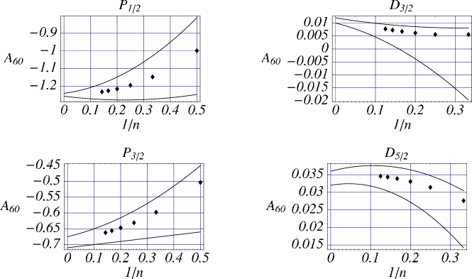
Figure 1: These graphs show exact and approximate values of the self-energy coefficient $A_{60}$—see Eq. (7). Exact values are represented by dots and can be found in Tables 1 and 2. The two curves of each graph represent the upper and lower limits of the approximation to $A_{60}$ provided by $\mathcal{A}_{3}$ in Eqs. (35), by taking into account the uncertainties in the coefficients of Table 8. For levels in hydrogen with principal quantum number $n\geq 10$, the uncertainty in $A_{60}$ deduced from these curves contributes to the uncertainty in the electron self energy (1) by less than 2 Hz. (The use of $1/n$ as the abscissa allows all large principal quantum numbers $n$ to be represented in the graphs.)

The coefficients $a_{i}$ of (35b) given in Table 8 can be useful to spectroscopy experiments that involve electronic levels with principal quantum numbers that are higher than those of Tables 1 and 2. In fact, the self energy of the electron of an hydrogenlike ion can be estimated through Eqs. (7), (8), (11) and (35), with $\mathcal{A}_{3}$ defined with the values of Table 8. Hydrogen has been and will be the subject of extremely precise spectroscopy experiments, which now reach the level of 1 Hz of uncertainty in transition frequencies. The uncertainty in the self energy (1) that comes from the uncertainties in the coefficients of Table 8 through (7) and (35) is comparable to the current experimental limit. In fact, the uncertainties in $\mathcal{A}_{3}$ in (35b) contribute to the self energy by less than $\pm$2 Hz for $\text{P}_{1/2}$ states with $n>7$, less than $\pm$1.6 Hz for $\text{P}_{3/2}$ states with $n>7$, less than $\pm$0.12 Hz for $\text{D}_{5/2}$ states with $n>8$, and less than $\pm$0.12 Hz for $\text{D}_{5/2}$ states with $n>8$ (precise values of $A_{60}$ for lower values of $n$ can be found in Tables 1 and 2).

Moreover, the coefficients of Table 8 can be useful to theoretical calculations. In fact, future values of $A_{60}$ for P and D states can be checked against the estimates provided by $\mathcal{A}_{3}$ in (35b)—see also the curves of Fig. 1.

VI Approximations of $A_{60}$ and of the Bethe logarithm

In addition to studying the dependence of $A_{60}(nl_{j})$ on $n$, as we did in the previous section for P and D states, it is interesting to analyze the behavior of $A_{60}(nl_{j})$ as a function of $l$, for $j=l-1/2$ and $j=l+1/2$. We conjecture that $A_{60}(\bar{n}l_{j})$, for $\bar{n}=l+1$ and $j=l\pm 1/2$, decreases as

$$A_{60}(\bar{n}l_{j})\underset{l\rightarrow\infty}{\sim}{\displaystyle\frac{c(j-l)}{l^{k}}}\quad\text{with $k\geq 3$},$$ (36)

where we probably have $k=4$ or $k=5$ [$c(1/2)$ and $c(-1/2)$ are two unspecified numbers]. The form (36) is motivated in this section.

We have also studied the asymptotic behavior of the Bethe logarithm $\ln k_{0}(\bar{n}l)$, because this is a quantity similar to the “relativistic Bethe logarithm” $A_{60}$, and because it yields a large contribution to the self energy [see Eqs. (7) and (8)]. We show in this section that the Bethe logarithm $\ln k_{0}(\bar{n}l)$, where $\bar{n}=l+1$, appears to behave asymptotically as $l^{-3}$. This result differs from the $l^{-7/2}$ asymptotic behavior of $\ln k_{0}(\bar{n}l)$ deduced from Eq. (B5) in (Erickson, 1977, p. 845). Extrapolations of the Bethe logarithm $\ln k_{0}(nl)$ as a function of $n$ have been obtained through the method described in the Appendix, and used in Ref. Kotochigova et al. (2002) for S, P and D states ($l=0$ to $2$).

We also postulate that the Bethe logarithm $\ln k_{0}(\bar{n}l)$, where $\bar{n}=l+1$, can be expanded in powers of $l^{-1}$ about $l=\infty$. In order to find the first five coefficients of such an expansion, we used the fitting procedure described in the Appendix. The resulting approximation reads:

$$l^{3}\times\ln k_{0}(\bar{n}l)\simeq$$

$$\Bigg{(}-0.056853(2)\displaystyle+\frac{0.02478(4)}{l}+\frac{0.0387(8)}{l^{2}}$$

$$\quad{}+\frac{-0.114(6)}{l^{3}}+\frac{0.16(2)}{l^{4}}\Bigg{)},$$

where $\bar{n}=l+1$, and where the neglected contribution is of order $l^{-5}$. This approximation should be valid for $l\rightarrow\infty$; nevertheless, it yields values of the Bethe logarithm that are both precise (see Fig. 2) and compatible with all the values of $\ln k_{0}(\bar{n}l)$ for $l=3,\ldots,19$ (taken from Ref. Drake and Swainson (1990)). For the $l\geq 20$ levels of hydrogen, the uncertainty in the result of approximation (VI) is negligible, when compared to the best experimental uncertainty in transition frequency measurements (about 1 Hz Biraben et al. (2001)).

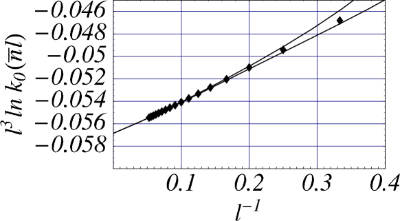
Figure 2: Comparison between exact values of $l^{3}\times\ln k_{0}(\bar{n}l)$ (dots) and the truncated asymptotic expansion of Eq. (VI) (zone between the two curves)—$\ln k_{0}(\bar{n}l)$ is the Bethe logarithm, and $\bar{n}=l+1$. The numerical values of the Bethe logarithms used in this graph Drake and Swainson (1990) are compatible with the values deduced from Eq. (VI), which are in the area between the two curves. The fact that the data points seem to converge toward a finite value ($\simeq-0.057$) as $l^{-1}\rightarrow 0$ supports the conjecture of a $l^{-3}$ asymptotic behavior of the Bethe logarithm $\ln k_{0}(\bar{n}l)$.

Moreover, we suggest that the orders of magnitude of the self-energy coefficient $A_{60}(nl_{j})$ and of the Bethe logarithm $\ln k_{0}(nl)$ do not depend on the principal quantum number $n$, i.e., the order of magnitude of a coefficient $A_{60}(nl_{j})$ is given by the order of magnitude of $A_{60}(\bar{n}l_{j})$, where $\bar{n}=l+1$ (and similarly for the Bethe logarithm). For $A_{60}$, this behavior is a generalization of what is observed for P, D, F and G states in Tables 1–4. For the Bethe logarithm, the fact that $\ln k_{0}(nl)$ and $\ln k_{0}(\bar{n}l)$ have the same order of magnitude can be observed for states with $l<n\leq 20$ by inspecting the results of Ref. Drake and Swainson (1990).

The expressions (36) and (VI) for the asymptotic behavior of $A_{60}(\bar{n}l_{j})$ and $\ln k_{0}(\bar{n}l)$, where $\bar{n}=l+1$, could thus be used for estimating the order of magnitude of the self energy (1)—with the help of Eqs. (7), (8), (11). Estimating the self energy correction (1) can be useful in high-precision spectroscopy experiments with large-$l$ levels. Thus, for instance, a recent experiment DeVries (2002) required evaluating the self energies of circular ($n=l+1$) states of orbital quantum number $l\simeq 30$. On the theoretical side, future calculations of $A_{60}(nl_{j})$ and $\ln k_{0}(nl)$ can be checked against the asymptotic behaviors of $A_{60}(\bar{n}l_{j})$ and $\ln k_{0}(\bar{n}l)$ that are described above.

Since the order of magnitude of $A_{60}(nl_{j})$ does not appear to depend on $n$, it is natural to represent it (for fixed $l$ and $j$) by the order of magnitude of either $\lim_{n\rightarrow\infty}A_{60}(nl_{j})$—largest possible $n$— or $A_{60}(\bar{n}l_{j})$—where $\bar{n}=l+1$ is the smallest $n$ possible for the angular momentum quantum number $l$. We chose the latter possibility for two reasons. First, small-$n$ values of $A_{60}(nl_{j})$ are available (see Tables 1–4). Second, future values of $A_{60}(nl_{j})$ for higher angular quantum numbers $l$ are likely to be obtained first for states where $n=l+1$, which is the smallest $n$ possible for a given angular momentum quantum number $l$. In particular, such states have simpler radial wavefunctions (the number of terms in the radial wavefunction of a state increases with $n-l$). And finally, circular states ($n=l+1$) are relevant to high-precision spectroscopy experiments (see, e.g., Ref. DeVries (2002)), whereas $n=\infty$ states are unphysical.

As mentioned above, we expect an asymptotic behavior of the form $l^{-k}$, with $k$ integer, for $A_{60}(\bar{n}l_{j})$ and for the Bethe logarithm $\ln k_{0}(\bar{n}l)$. Such a functional form is motivated by the fact that all the $A_{ik}(nl_{j})$ coefficients of the self-energy function $F$ in Eq. (5) can be expanded in power series of $1/n$ and $l^{-1}$, except maybe for the two coefficients related to this section, $A_{60}$ and $A_{40}$, where the latter is a function of the Bethe logarithm [see Eq. (8)]. (We suppose that $A_{60}$ and $A_{40}$ can also be expanded in such a series.) This can for instance be checked with the formulas for $A_{ik}(nl_{j})$ reviewed in Ref. (Mohr and Taylor, 2000, p. 468), with the help of Eq. (II) for $A_{61}(nl_{j})$, where $\Psi(n+1)$ can be expanded in powers of $1/(n+1)$ (Abramovitz and Stegun, 1972, § 6.3.18).

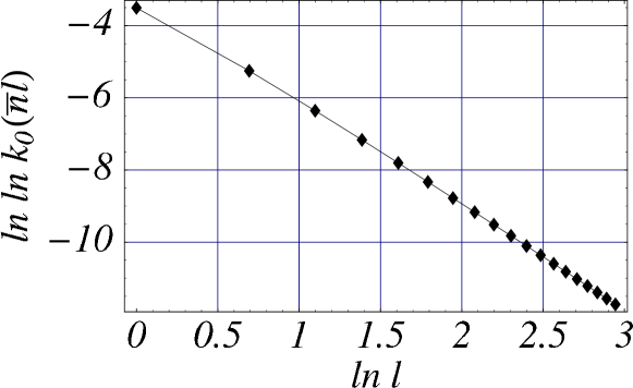
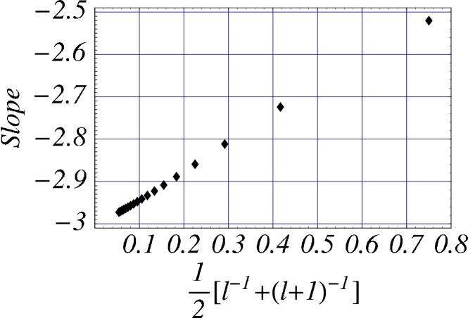
Figure 3: Upper graph: log-log plot of the Bethe logarithm $\ln k_{0}(\bar{n}l)$, where $\bar{n}=l+1$. Lower graph: slope between two successive points of the log-log plot. The limit slope of $-3$ as $l\rightarrow\infty$ observed in the lower graph indicates that the Bethe logarithm $\ln k_{0}(\bar{n}l)$ behaves asymptotically as $l^{-3}$. This confirms what is observed in Fig. 2. (The abscissa of the points in the lower graph is chosen so as to produce a graph from which the limit slope of the upper graph as $l\rightarrow\infty$ can be easily deduced.)

The $l^{-3}$ behavior of the Bethe logarithm $\ln k_{0}(\bar{n}l)$, where $\bar{n}=l+1$, is suggested by Fig. 2. The points of this graph, which represent

$$l^{3}\times\ln k_{0}(\bar{n}l),$$ (38)

appear to converge toward a limit ($\simeq-0.057$) as $l^{-1}\rightarrow 0$. We checked the $l^{-3}$ behavior deduced from the study of Eq. (38) by calculating the slope of a log-log plot of the Bethe logarithm $\ln k_{0}(\bar{n}l)$ (with numerical values taken from Ref. Drake and Swainson (1990)). The result, shown in Fig. 3, indicates that the Bethe logarithm does indeed behave asymptotically as $l^{-3}$; this coincides with the conclusion from Fig. 2.

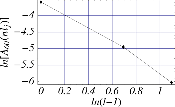
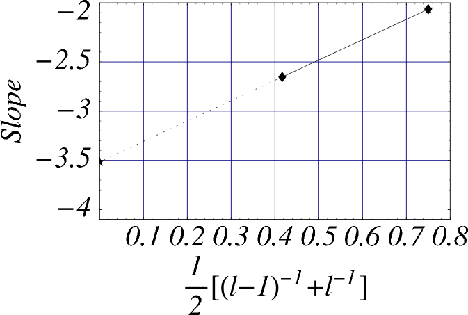
Figure 4: Upper graph: log-log plot of the self-energy coefficient $A_{60}(\bar{n}l_{j})$, where $\bar{n}=l+1$ and $j=l+1/2$. Lower graph: slope between two successive points of the log-log plot (solid line) and extrapolation to $l\rightarrow\infty$ (dashes). By analogy with the graphs similarly obtained for the Bethe logarithm in Fig. 3, we conclude that for $j=l+1/2$, $A_{60}(\bar{n}l_{j})$ behaves asymptotically as $l^{-k}$ with $k\geq 3$ and, probably, $k=4$ or $k=5$. The values of $A_{60}$ are taken from Tables 2–4.

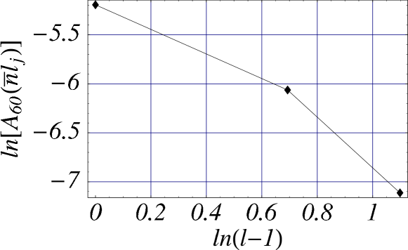
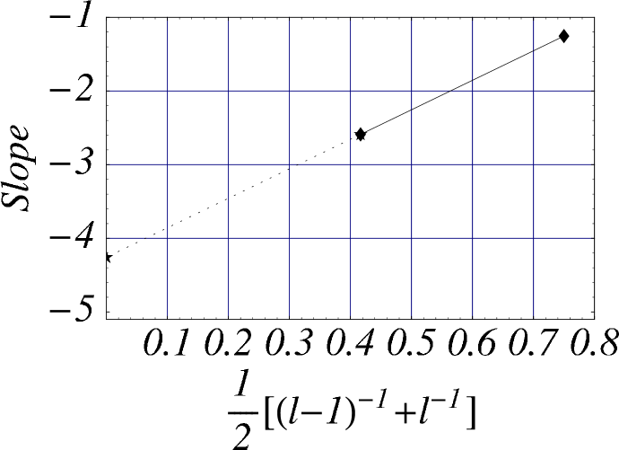
Figure 5: Upper graph: log-log plot of the self-energy coefficient $A_{60}(\bar{n}l_{j})$, where $\bar{n}=l+1$ and $j=l-1/2$. Lower graph: slope between two successive points of the log-log plot (solid line) and extrapolation to $l\rightarrow\infty$ (dashes). By analogy with the graphs similarly obtained for the Bethe logarithm in Fig. 3, we conclude that for $j=l-1/2$, $A_{60}(\bar{n}l_{j})$ behaves asymptotically as $l^{-k}$ with $k\geq 3$ and, probably, $k=4$ or $k=5$. The values of $A_{60}$ are taken from Tables 2–4.

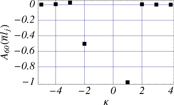
Figure 6: This graph shows values of the self-energy coefficients $A_{60}(\bar{n}l_{j})$, where $\bar{n}=l+1$, as a function of the Dirac quantum number $\kappa$, where $\kappa$ is defined in (2). The large value $A_{60}(1S_{1/2})\simeq-31$ is not represented here. This plot shows that for S and P states ($\kappa=-2$, $-1$ and $1$), the $A_{60}$ coefficient exhibits an exceptional behavior; such an exceptional behavior is also found in the self-energy coefficient $A_{61}$ in Eq. (II), which is known analytically.

It is possible to use the procedure depicted in Fig. 3 to estimate the integer exponent $k$ of an asymptotic behavior $l^{-k}$ for the relativistic Bethe logarithm $A_{60}(\bar{n}l_{j})$, where $\bar{n}=l+1$ and $j=l\pm 1/2$. In fact, it is reasonable to use the Bethe logarithm $\ln k_{0}(\bar{n}l)$ as a guide for studying the relativistic Bethe logarithm $A_{60}$. Thus, the procedure depicted in Fig. 3 was applied to the self-energy coefficient $A_{60}(\bar{n}l_{j})$; we obtained the asymptotic behavior presented at the beginning of this section, and in particular in Eq. (36). The graphs supporting (36) are given in Fig. 4 for with states with $j=l+1/2$, and in Fig. 5 for states with $j=l-1/2$. Each of these graphs uses only three values of $A_{60}$ (D, F and G states); even though this is a relatively small number of values compared to the number of available values of the Bethe logarithm, the behavior of the first few data points in Fig. 3 justifies using only a few small-$l$ values in order to predict the asymptotic behavior of $A_{60}(\bar{n}l_{j})$ for $l\rightarrow\infty$.

The values of the $A_{60}$ coefficient of S and P states were not used in obtaining Eq. (36), because it is convenient to treat the orders of magnitude of the $A_{60}$ coefficient of these states separately from the orders of magnitude of higher-$l$ states; Fig. 6 illustrates this point. We note that the self-energy coefficient $A_{61}$ also exhibits an exceptional behavior for S and P states (see, e.g., Eq. (4.4a) in Erickson and Yennie (1965a)). As an additional consequence, estimating the coefficient $c$ of the asymptotic form of $A_{60}$ in Eq. (36) would require use of states with orbital angular momentum quantum number $l\geq 2$ (D, F, etc.).

The possible values of the exponent $k$ in Eq. (36) deduced from both the graphs of Fig. 4 and of Fig. 5 are compatible with each other ($k\geq 3$ with, probably, $k=4$ or $k=5$). It is indeed expected that the asymptotic form of $A_{60}(\bar{n}l_{j})$ be the same for $j=l+1/2$ and $j=l-1/2$, as can be seen from the numerical values for D, F and G states found in Tables 2–4. More precise estimates of the asymptotic exponent $k$ in Eq. (36) can be obtained through the procedure we used in Figs. 4 and 5, as soon as additional values of $A_{60}(\bar{n}l_{j})$, with $\bar{n}=l+1$ are available.

According to the results of this section, the “relativistic Bethe logarithm” $A_{60}(\bar{n}l_{j})$ decreases at least as fast (and probably one or two powers faster), as a function of $l$, than the Bethe logarithm $\ln k_{0}(\bar{n}{l})$. Such a behavior is also found in the (Dirac-Coulomb) energy of hydrogen and hydrogenlike ions. Thus, the Dirac-Coulomb energy of an electron bound to a nucleus of charge number $Z$ is (see, e.g., (Mohr and Taylor, 2000, p. 466))

$$E_{nj}=\left[1+\frac{(Z\alpha)^{2}}{(n-\delta)^{2}}\right]^{-1/2},$$ (39)

where

$$\delta=(j+1/2)-\sqrt{(j+1/2)^{2}-(Z\alpha)^{2}}.$$

According to (39), an electron in a circular state $\bar{n}l_{j}$ with $j=l+1/2$ (and $\bar{n}=l+1$) has an energy

$$E_{\bar{n},l+\frac{1}{2}}=\sqrt{{1-[Z\alpha/(l+1)]^{2}}}.$$ (40)

In the Taylor expansion (in $Z\alpha$) of this energy, the asymptotic behavior of the coefficient of $(Z\alpha)^{2k}$ is given by $l^{-2k}$ (this conclusion also holds for circular state $\bar{n}l_{j}$ with $j=l-1/2$). Thus, for circular states, successive relativistic corrections to the nonrelativistic energy of a bound electron fall off faster and faster with the orbital quantum number $l$, with two additional powers of $l^{-1}$ for each order in $(Z\alpha)^{2}$. If this rule applies to the coefficients of the self-energy expansion (7), the asymptotic form of $A_{60}(\bar{n}l_{j})$ as $l\rightarrow\infty$ should be $l^{-4}$; in fact, the lower-order coefficient $A_{40}(\bar{n}l_{j})$ decreases as $l^{-2}$, as can be seen in Eq. (8). On the other hand, since $A_{60}(nl_{j})$ can be considered as a relativistic correction to the Bethe logarithm, applying the above rule yields an asymptotic form in $l^{-5}$ for $A_{60}(\bar{n}l_{j})$, since the Bethe logarithm behaves as $l^{-3}$, as described in this section. These observations are fully compatible with the graphs of Figs. 4 and 5, from which the asymptotic form (36) of $A_{60}(\bar{n}l_{j})$ was deduced (with an exponent $k$ probably equal to 4 or 5).

VII Checks of the $A_{60}$ coefficients

We have checked our analytic results for $A_{60}$ (cf. Tables 1–4) by an independent method: the analytic results were compared to values deduced from non-perturbative, numerical calculations of the self energy (1). We have used the numerical self-energy values of Refs. Le Bigot et al. (2001); Jentschura et al. (2001); Indelicato and Mohr (1998a, b); Mohr and Kim (1992); Mohr (1992), as well as new values Le Bigot et al. , which extend the results of Ref. Le Bigot et al. (2001) to smaller nuclear charge numbers $Z$ (to $Z$ between 10 and 25). In most cases, the checks that we detail below confirm the values of $A_{60}$ reported in Tables 1–4, to a relative precision of about 15 %. The few exceptions are the following. For 2P states, the numerical values of the self-energy confirm the results of Table 1 to about 1 %. For $n\text{D}_{3/2}$ states with $n=3,\ldots,8$, the non-perturbative self-energy results yield $A_{60}(n\text{D}_{3/2})=0.005(10)$, in agreement with the results of Table 2. And finally, we did not check $A_{60}(8\text{D}_{5/2})$ in Table 2 by using non-perturbative self-energy values because no such values are available for the $8\text{D}_{5/2}$ state. However, as depicted in Fig. 1, the value of $A_{60}(8\text{D}_{5/2})$ reported here appears to fit well within the series of $A_{60}(n\text{D}_{5/2})$ values for $n=3,\ldots,7$ (see Table 2).

(a)     

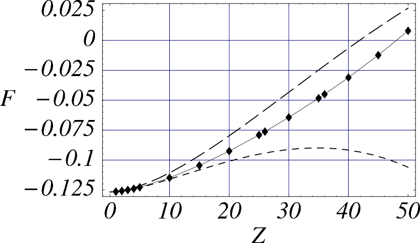
(b)        

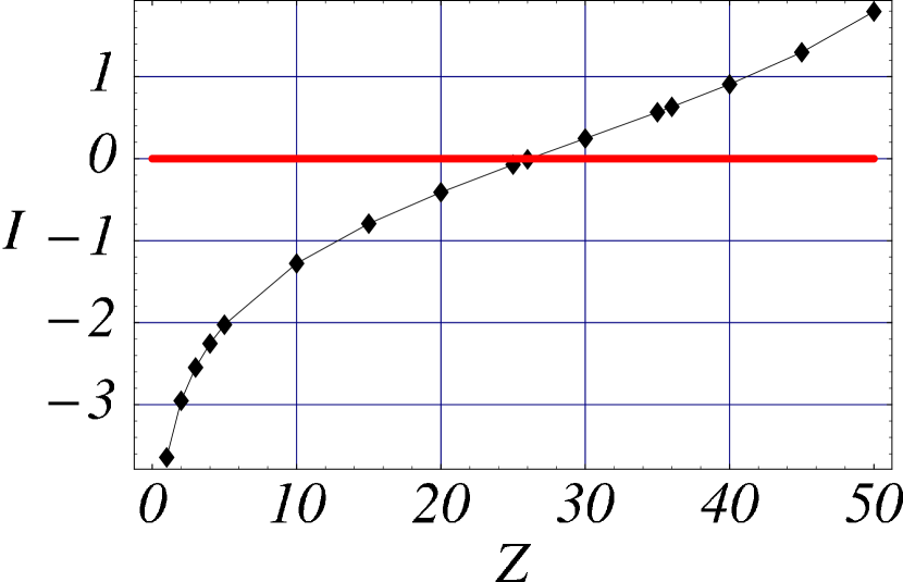
Figure 7: Figure (a) shows exact and approximate values of the (scaled) self energy $F$ of a $2\text{P}_{1/2}$ electron [see Eq. (1)]. Exact values are given on the solid line. The two-coefficient approximation (41) is represented by long dashes. The three-coefficient approximation (42) uses the value of $A_{60}(2\text{P}_{1/2})$ that we provide in Table 1, and is indicated by short dashes. Figure (b) displays the improvement provided by the inclusion of $A_{60}$ in the self-energy approximation, as measured by the function $I$ in Eq. (43); negative values of $I$ indicate that including $A_{60}$ improves the approximation.

(a)     

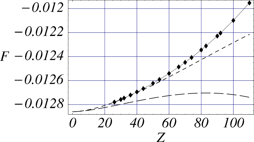
(b)         

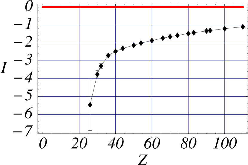
Figure 8: These two figures represent respectively the same quantities as those found in Fig. 7, but for the $5\text{G}_{7/2}$ level instead of the $2\text{P}_{1/2}$ level. The fact that curve (b) contains negative values of $I$ [see Eq. (43)] indicates that the three-order approximation (42) to the self energy (7) is better than the two-order approximation (41), at least over the range of nuclear charge numbers $Z=25$–$110$. The three-order approximation (42) uses the value of $A_{60}(5G_{7/2})$ reported in Table 4.

The first check that we applied consisted of comparing the numerical, exact results for $F$ to two of its successive approximations. The first approximation, $F^{(2)}(Z\alpha)$, includes the two dominant and already-known coefficients $A_{40}$ (8) and $A_{61}$ (II) of expansion (7):

$$F^{(2)}(Z\alpha)=A_{40}+(Z\alpha)^{2}A_{61}\ln(Z\alpha)^{-2},$$ (41)

and the second approximation, $F^{(3)}$, includes in addition the next-order contribution reported in this paper:

$$F^{(3)}(Z\alpha)=A_{40}+(Z\alpha)^{2}\left[A_{61}\ln(Z\alpha)^{-2}+A_{60}\right].$$ (42)

For a given electronic level $nl_{j}$, one expects that for low $Z$, the curve of the higher-order approximation $F^{(3)}(Z\alpha)$ be closer to the curve of $F(Z\alpha)$ than $F^{(2)}(Z\alpha)$. In order to check this, we plotted the quantity

$$I(Z\alpha)=\ln\left|\frac{F(Z\alpha)-F^{(3)}(Z\alpha)}{F(Z\alpha)-F^{(2)}(Z\alpha)}\right|,$$ (43)

which should go to $-\infty$ as $Z\rightarrow 0$, as can be seen from Eq. (7). In (43), the purpose of the logarithm is only to obtain more legible graphs; a value of $I$ lower than zero indicates that including $A_{60}$ in the approximation of $F$ improves the lower-order approximation. For the states of Tables 1–4, graphs of (43) are compatible with their expected behavior [$I(Z\alpha)$ is negative for $Z$ sufficiently close to zero, and is consistent with a $-\infty$ limit]. Figures 7 and 8 show this behavior for two electronic states.

Moreover, the improvement provided by the inclusion of $A_{60}$ in the approximation for $F$ becomes greater as the total angular momentum $j$ increases: for given $n$ and $Z$, the improvement function (43) decreases as $j$ increases; this behavior can observed by comparing Figs. 7 and 8. Similarily, the range of $Z$ for which approximation $F^{(3)}$ is better than $F^{(2)}$ increases with increasing $j$. In the worst of the cases considered here ($j=1/2$), approximation $F^{(3)}$ is better than $F^{(2)}$ up to $Z\simeq 25$. As shown in Fig. 8, for a high-$j$ level such as $5\text{G}_{7/2}$, the higher-order approximation $F^{(3)}$ is better than $F^{(2)}$ even up to $Z=110$.

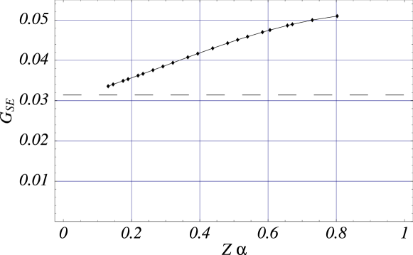
Figure 9: Plot (solid line) of numerical values of the remainder $G_{\text{SE}}(4\text{D}_{5/2},Z\alpha)$ of the self energy (5); the dashed line indicates the value of $A_{60}(4\text{D}_{5/2})\simeq 0.0314$ reported in this paper (see Table 2). By definition, the coefficient $A_{60}$ can be obtained as the limit (6) of $G_{\text{SE}}$ as $Z\alpha\rightarrow 0$. This plot shows that the value of $A_{60}$ extracted from numerical self-energies is consistent with the value obtained by the calculations presented in this paper. We made identical observations for all the states of Tables 1–4.

The second check consisted in estimating $A_{60}$ from the numerical values of the self energy (1). For all the electronic levels $nl_{j}$ studied here (except for $8\text{D}_{5/2}$), we have plotted the function $G_{\text{SE}}(nl_{j},Z\alpha)$ of (5); this is made possible by the fact that all the coefficients of (5) are (analytically) known for any state Erickson and Yennie (1965a, b), except for the Bethe logarithm, which has been numerically evaluated for many states, including the ones we consider here Haywood and Morgan III (1985); Drake and Swainson (1990); Forrey and Hill (1993); Goldman and Drake (2000). As indicated in (6), the limit of the remainder $G_{\text{SE}}(nl_{j},Z\alpha)$ as $Z\alpha\to 0$ is by definition $A_{60}(nl_{j})$. We have estimated this limit both visually and by fitting $G_{\text{SE}}(nl_{j},Z\alpha)$ with various choices of non-zero higher-order terms. A typical curve for $G_{\text{SE}}(Z\alpha)$ is shown in Fig. 9. The estimates of $A_{60}$ obtained by these procedures confirm the independent analytic results of Tables 1–4 to a typical accuracy of 10–20 %, with a few exceptions. Thus, for 2P levels, plotting $G_{\text{SE}}$ as in Fig. 9 allowed us to confirm the values of $A_{60}(2{\text{P}}_{j})$ in Table 1 to a precision of about 1 %. This higher precision is obtained by using the self energies of 2P states obtained in Ref. Jentschura et al. (2001) for values of $Z\alpha$ close to zero ($Z=1,\ldots,5$): such low-$Z$ self energies are well-suited to an evaluation of $A_{60}$ by the limit (6). Plotting $G_{\text{SE}}$ for $\text{D}_{3/2}$ states lead to $A_{60}(n\text{D}_{3/2})=0.005(10)$ for $n=3,\ldots,8$, in agreement with Table 2. Finally, since no non-perturbative self-energy (1) is available for $8\text{D}_{5/2}$ states, we were not able to independently obtain $A_{60}(8\text{D}_{5/2})$ by using such values.

As a by-product of our work with graphs of $G_{\text{SE}}(nl_{j},Z\alpha)$, we estimate the self-energy remainder $G_{\text{SE}}(nl_{j},\alpha)$ relevant to hydrogen ($Z=1$) to be 0.030(5) for $3\text{D}_{5/2}$ and $4\text{D}_{5/2}$ states [see Eq. (5)]; this is larger than the estimate of 0.00(1) given in Ref. (Mohr and Taylor, 2000, p. 468). These two new values change the previous estimate of the self energy of $3\text{D}_{5/2}$ and $4\text{D}_{5/2}$ states through Eq. (7) by a relatively large amount, compared to the current best experimental uncertainty in transition frequencies (about 1 Hz Biraben et al. (2001)). Thus, a variation of 0.03 in $G_{\text{SE}}(3\text{D}_{5/2},\alpha)$ in (5) corresponds to a variation of about 50 Hz in the self energy correction (1) of the $3\text{D}_{5/2}$ level in hydrogen. The same variation in $G_{\text{SE}}(4\text{D}_{5/2},\alpha)$ induces a variation of about 20 Hz in the self energy of the $4\text{D}_{5/2}$ level in hydrogen; on the other hand, this latter change is small compared to the uncertainty of the relevant measurements considered in Ref. Mohr and Taylor (2000).

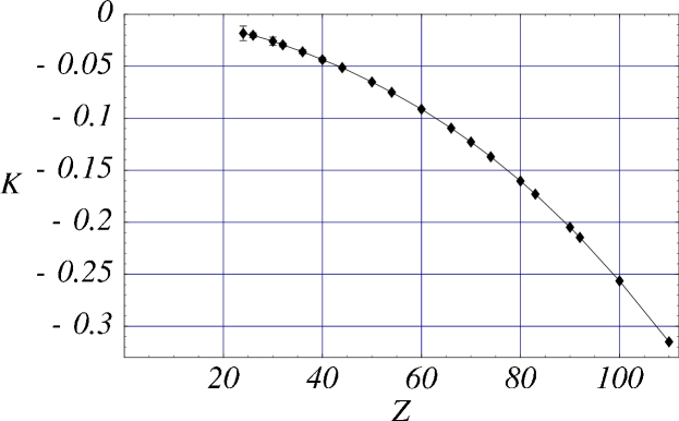
Figure 10: Plot of the function $K$ in Eq. (47) for the $5\text{F}_{7/2}$ and $5\text{F}_{5/2}$ states. The limit of this function as $Z\rightarrow 0$ must be zero if the coefficients $A_{60}$ of Tables 1–4 agree with exact, numerical values of the self energy. The curve displayed here indicates that the two values of $\Delta_{\text{fs}}A_{60}(5F)$ in Eq. (46) obtained independently from Table 3 and from non-perturbative self energies (1) [via Eqs. (7), (8), (11c), (44) and (VII)] do not differ by more than about 3 %.

As a third and last check, we used the numerical, exact values of $F$ in order to study the following difference between remainders $G_{\text{SE}}$ [see Eqs. (5) and (7)]:

$$\Delta_{\text{fs}}G_{\text{SE}}(nl,Z\alpha)=G_{\text{SE}}(nl_{l+1/2},Z\alpha)-G_{\text{SE}}(nl_{l-1/2},Z\alpha),$$ (44)

where, by definition of $A_{60}$ (6),

$$\lim_{Z\alpha\rightarrow 0}\Delta_{\text{fs}}G_{\text{SE}}(nl,Z\alpha)$$

$$= A_{60}(nl_{l+1/2})-A_{60}(nl_{l-1/2})$$

$$= \Delta_{\text{fs}}A_{60}(nl)\,,$$ (46)

which denotes a quantity associated to the fine-structure. The numerical evaluation of this limit is interesting: for the states of Tables 1–4, the numerical results for $F$ yield values of $\Delta_{\text{fs}}A_{60}(nl)$ that are more accurate than our numerical estimates of the two individual terms $A_{60}(nl_{l+1/2})$ and $A_{60}(nl_{l-1/2})$. Our analytic values for $\Delta_{\text{fs}}A_{60}$ in Eq. (46) were checked by plotting

$$K(Z)=\frac{\Delta_{\text{fs}}G_{\text{SE}}(nl,Z\alpha)}{\Delta_{\text{fs}}A_{60}(nl)}-1,$$ (47)

where $\Delta_{\text{fs}}G_{\text{SE}}(nl,Z\alpha)$ was calculated from the numerical values of $F$ [see Eq. (7) and the coefficients reproduced in Sec. II], and where the value of $\Delta_{\text{fs}}A_{60}(nl)$ in Eq. (46) was deduced from the analytic results of Tables 1–4. If the numerical and analytic estimates of $\Delta_{\text{fs}}A_{60}(nl)$ do agree, the function (47) goes to zero as $Z\rightarrow 0$. This is indeed consistent with what we observed; figure 10 provides an example of this behavior. We confirm the values of $\Delta_{\text{fs}}A_{60}(nl)$ in Eq. (46) that can be immediately deduced from Tables 1–4. The analytic results for $\Delta_{\text{fs}}A_{60}(nl)$ are thus found to be consistent with the numerical data for $\Delta_{\text{fs}}G_{\text{SE}}$; the level of confirmation is 5–10 % [relative to $\Delta_{\text{fs}}A_{60}(nl)$] for P and D states (1 % for the 2P states, and $8\text{D}$ states not included, for the reason mentioned above), 3 % for F states, and 1% for G states.

This represents an improvement over the accuracy of $A_{60}(nl_{j})$ obtained by the previous check. This improvement comes evidently from the fact that the relative deviation of $\Delta_{\text{fs}}G_{\text{SE}}$ in Eq. (44) from $\Delta_{\text{fs}}A_{60}$ in Eq. (46) is small over the whole range $0<Z\leq 110$, compared to the relative deviation

$$\frac{G_{\text{SE}}(nl_{j},Z\alpha)}{A_{60}(nl_{j})}-1,$$ (48)

of $G_{\text{SE}}$ [see Eq. (5)] from $A_{60}(nl_{j})$ in Eq. (6)—with $j=l+1/2$ or $j=l-1/2$. As a consequence, the uncertainty in the numerical evaluation of the limit of (47) as $Z\rightarrow 0$ is relatively small. Figure 10 shows an example of the smallness of the contributions to $\Delta_{\text{fs}}G_{\text{SE}}$ that go beyond $\Delta_{\text{fs}}A_{60}$. Moreover, we have observed that the higher the angular momentum $l$, the smaller the values of the deviation (47), hence the stronger confirmation of our values of $\Delta_{\text{fs}}A_{60}(nl)$ for high orbital angular momenta.

VIII Summary of Results

This paper contains results that are relevant to the self energy of a non-S electron bound to a point nucleus of charge number $Z$. We provided estimates and values (see also Ref. Jentschura et al. (2003)) for the first two non-analytically-known contributions to the self-energy expansion (5), namely the Bethe logarithm $\ln k_{0}(nl)$ and the so-called $A_{60}(nl_{j})$ coefficient, which can be viewed as a relativistic Bethe logarithm. The main numerical results are contained in Tables 1–4, in Eq. (35) and Table 8, in Eq. (36) and in Eq. (VI). We have also conjectured, in Sec. VI, that the relativistic Bethe logarithm $A_{60}(nl_{j})$ does not strongly depend on the principal quantum number $n$. In addition to this, we note that the orders of magnitude of $A_{60}(n\,l_{l-1/2})$ and $A_{60}(n\,(l+1)_{l+3/2})$ are the same (for a given set of quantum numbers $n$ and $l>1$), in Tables 1–4. These results, taken together, yield in particular the best available approximations of the self energy in hydrogen and light hydrogenlike ions, except for $n=1$ and $n=2$ levels Jentschura et al. (1999a); Jentschura et al. (2001) (see also Sec. VII); such an approximation can be obtained through Eqs. (1) and (7).

Calculating $A_{60}$ has been a challenge since the seminal work of Bethe Bethe (1947) on the dominant self-energy coefficients of S states [see Eqs. (7) and (1)]. Details of the method we used were described in Sec. III and IV. As discussed in Sec. VII, including the coefficients $A_{60}$ reported in Tables 1–4 in a (truncated) expansion of the self energy improves its accuracy over a large range of nuclear charge numbers $Z$.

We checked our calculations of $A_{60}$ by both analytic and numerical means. The so-called $\epsilon$ method, which we have employed (see Sec. III), makes divergences appear in the low- and high-energy contributions to $A_{60}$, as the scale-separating parameter $\epsilon$ between these two contributions goes to zero. We have observed that, as required, these divergences cancel when the two parts are added. Moreover, our calculations correctly reproduced the known lower-order coefficients $A_{40}$ and $A_{61}$. We have also checked our results for $A_{60}$ against numerical values of the self energy, and were able to confirm them by this independent method to the level of about 15 % (except for $\text{D}_{3/2}$ states, as explained in Sect. VII).

Obtaining results for $A_{60}$ required extending (analytically) the angular algebra developed for 2P states Jentschura and Pachucki (1996) to higher angular momenta. Techniques of numerical convergence acceleration of series Jentschura (1999); Jentschura et al. (1999b); Aksenov et al. (2003) were instrumental in evaluating the parts of $A_{60}$ that could not be analytically calculated. The recent analytic calculations of Ref. Le Bigot et al. (2001) enabled us to obtain with a high precision the self energy (1) of electrons with high ($j>3/2$) angular momentum, for various values of the nuclear charge number $Z$; the new calculations that we have performed required the use of massively parallel computers, and thousands of hours of computing time. (These numerical data, which have been used for the plots in Figs. 8–10, will be presented in detail elsewhere Le Bigot et al. .) We have also collected the most recent available values of the self energy. This provided us with independent values of the $A_{60}$ coefficients, extracted from the numerical self-energies, thus allowing us to check the analytic results presented in Tables 1–4 (see Sec. VII).

Severe cancellations appeared, between different contributions to $A_{60}$ (in addition to the cancellation of the $\epsilon$-parameter divergences): for some of the atomic states investigated, the absolute magnitude of the $A_{60}$ coefficients is as small as $10^{-3}$, whereas the largest individual contribution to $A_{60}$, when following the classification of the corrections according to Refs. Jentschura and Pachucki (1996); Jentschura et al. (1997), is of the order of $10^{-2}$ or larger for all atomic states discussed here (see also Tables 6 and 7).

Future calculations of the Bethe logarithm $\ln k_{0}(nl)$ and of the relativistic Bethe logarithm $A_{60}(nl_{j})$ could also fruitfully be compared to the estimates given by Eqs. (35), (36) and (VI), and Table 8. The results presented in this paper also allow one to perform checks of future exact self-energies obtained by numerical methods, by comparing their values to the three-term self-energy approximation (42) provided here for P and higher-$l$ states. The values of $A_{60}$ in Tables 1–4 can be of interest for analyzing the Lamb shift of highly-excited (high-$n$ and high-$l$) electronic states in recent de Beauvoir et al. (1997); Schwob et al. (1999, 2001); DeVries (2002) and future high-precision spectroscopy experiments. The results of Sect. IV–VI also provide the best available self-energy approximation for many states $nl_{j}$ and nuclear charge numbers $Z$ (see Sec. VII); these approximations can for instance be useful in evaluating the contribution of QED effects in atoms Feldman et al. (1990); Parente et al. (1994); Beck (1992); Sugar et al. (1989) or molecules Pyykkö et al. (2001).

Appendix: local fits

This appendix describes a fitting procedure which is designed to extract “local” numerical quantities from a set of data points, and to allow one to assess the numerical uncertainty associated to these quantities. A partial sketch of this procedure was first introduced in Ref. Mohr (1975). Here, “local” refer for instance to the evaluation of a perturbation expansion about one abscissa; the purpose of the method presented here is to perform fits that are local to an abscissa of interest, as opposed to finding the best global fit of some data points. We thus used it in order to obtain asymptotic coefficients for $A_{60}(nl_{j})$ for P and D states in Sec. V (see Table 8), as well as the asymptotic expansion of the Bethe logarithm $\ln k_{0}(nl)$ in Eq. (VI)—in these applications, the quantities evaluated are local to either $n=\infty$ or $l=\infty$. This method can in principle be applied to many other problems that require local fits.

In order to describe the local-fit procedure, we take the evaluation of the limit

$$\lim_{l\rightarrow\infty}l^{3}\times\ln k_{0}(\bar{n}l)$$ (49)

as an example—here, we have $\bar{n}=l+1$ and $\ln k_{0}({n}l)$ is the Bethe logarithm (II). This limit was evaluated as $-0.056853(2)$ [see Fig. 2 and Eq. (VI)].

Figures 2 and 11 contain data points which are relevant to (49): we have plotted

$$l^{3}\times\ln k_{0}(\bar{n}l)$$ (50)

as a function of $l^{-1}$ (with values of the Bethe logarithm found in Ref. Drake and Swainson (1990)). The limit (49) can visually be estimated from the data points in Fig. 2 to be $-0.057(1)$.

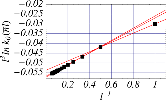
Figure 11: This figure shows the lines going through a few pairs of successive data points (50)—see also Fig. 2. Each of these lines is a local approximation to the curve underlying the data points. Each line yields an estimate of the limit (49) of the data points as $l^{-1}\rightarrow 0$ (this estimate is at the intersection of the line with the $l^{-1}=0$ axis). Fig. 12 graphically displays these estimates.

Figure 12: This figure shows the estimates of limit (49) obtained through the two-point fits of Fig. 11. From this graph, we limit (49) to be $-0.0568(1)$, which is more precise than, and coherent with the value $-0.057(1)$ obtained from the original data points (50) in Figs. 2 and 11. The limit estimates are plotted along the vertical direction, while the abscissa associated to an estimate is the average abscissa of the two data points of Fig. 11 that were used in producing it.

In order to improve over the estimate $-0.057(1)$ for (49), we fit (exactly) each pair of two consecutive points (50) in Fig. 2 with a line, as depicted in Fig. 11. Each of the fitting lines in Fig. 11 gives an estimate of limit (49) by extrapolation to $l^{-1}=0$ (intersection of the line with the $l^{-1}=0$ axis). Figure 12 contains each of these estimates, as a function of the average abscissa of the two points that were used in obtaining it. Because the curve in Fig. 12 is relatively flatter than the curve in Fig. 11, we can estimate limit (49) with an improved uncertainty; thus, we deduce from Fig. 12 the value $-0.0568(1)$ for the limit (49) that we are studying, which is coherent with the previous estimate $-0.057(1)$.

Figure 13: From the lower to the higher curve: estimates of limit (49) obtained through fits of the data points (50) with polynomials of degree $1$ (see also Fig. 12), $3$ and $5$ (see also Fig. 14). Fitting the data points (50) of Fig. (11) with 1 to 6 points yielded mutually coherent estimates of limit (49) with an exponentially decreasing error.

Figure 14: This figure shows estimates of limit (49) obtained by fitting the data points (50) in Fig. 11 with fifth-degree polynomials (in $l^{-1}$). The high relative stability of the estimates as $l^{-1}\rightarrow 0$ allowed us to give the precise value $-0.056853(2)$ in Eq. (VI) for limit (49).

Figure 15: This figure displays estimates of limit (49) obtained by fitting the data points (50) in Fig. 11 with a eigth-degree polynomials (in $l^{-1}$). It should be compared to Fig. 14, which gives a more accurate estimate of limit (49) by fitting sequences of only six data points. The accuracy of the local fits performed here first increases with the order of the local approximations to the data points (50) (see Fig. 13), and then eventually decreases (compare this plot to Fig. 14).

This better estimate $-0.0568(1)$ of limit (49) can be further improved by continuing to increase the number $p$ of data points (50) included in local fits of the data. Thus, for an increasing number $p$ of data points, we fitted (exactly) each set of $p$ successive points (50) in Fig. 11 with a polynomial of degree $p-1$ (linear combination of the functions $1$, $l^{-1}$,…, $l^{-(p-1)}$), and represented the value of the polynomial extrapolated to $l^{-1}=0$ as a function of the average abscissa of the $p$ points. Fig. 13 depicts this process. The plotted values are estimates of the limit (49) obtained with higher and higher-order (local) fits of the data points (50). In Fig. 13, the abscissa of each estimate is the average of the abscissas $l^{-1}$ of the fitted data points (50). We observed that the curves so obtained become exponentially flat, in the sense that their relative amplitude become exponentially smaller and smaller—until the uncertainties of individual estimates become important, as described below. This fact, which is illustrated in Fig. (13), allowed us to obtain more and more accurate estimates of limit (49).

The most accurate value that we obtained for limit (49) through the local-fit procedure described here is $-0.056853(2)$ [see Eq. (VI)], as is illustrated in Fig. 14. This limit was obtained by fitting each sequence of $p=6$ data points with a fifth-degree polynomial. Fits of the data points (50) with larger numbers of data points display more irregular estimate curves; this can for instance be seen by comparing Fig. 14 with Fig. 15.

As we have seen above, the uncertainty in the fitted value can be evaluated by visually prolongating the fitting curves (i.e., curves such as those of Figs. 12–15). Another uncertainty must in general be taken into account in order to obtain a reliable estimate for the fitted quantity: the uncertainty in the data points. All the curves presented in this appendix do contain error bars that reflect the uncertainties in the estimates of (49) that come from the uncertainties in the data points (50). We evaluated the uncertainty associated to each fit of $p$ data points (50) by calculating three fits: a fit with the middle values of the ordinates, a fit with the higher values, and a fit with the lower values; the three estimates of the fitted quantity (49) obtained through this procedure define an estimate with an error bar (see, e.g., Fig. 15). Other ways of estimating the uncertainty in the fit result can be used; a good choice of uncertainty evaluation yields successive estimates of the fitted quantity that are compatible with a smooth curve of estimates [see, e.g., Fig. 15, where the less precise estimates of limit (49) lie in the prolongation of the more precise values, which are on the right of the plot].

One of the advantages of the local-fit method presented in this appendix is that data points that are located far from the abscissa of interest ($l^{-1}=0$, here) can fruitfully be used in evaluating the fitted quantity [limit (49), in our example]. Thus, as Fig. 15 illustrates, data points (50) with “large” abscissas can yield more precise estimates of limit (49) than data points with small abscissas. This behavior is particularly useful when data points in the region of interest have relatively large uncertainties.

The procedure detailed in this Appendix also allows one to study the quality of lists of numerical results that should lie on a smooth curve, but whose coherence is not obvious through a simple inspection or plot of the values. In fact, curves such as those found in Figs. 12–15 can be very sensitive to small errors in a list of numerical values. We have not noticed such errors in the $A_{60}$ values of Tables 1 and 2 while evaluating the asymptotic coefficients reported in Table 8; this provided an additional check of the values reported in these tables (see also Sec. VII).

The local-fit method described here is not restricted to the asymptotic study of the Bethe logarithm that we have used as an example. In general, it can yield precise estimates of quantities that are local to a set of data point [such as limit (49)], including, for instance, perturbation coefficients of non-analytic expansions [e.g., Eq. (5)].

References

- Biraben et al. (2001) F. Biraben, T. W. Hänsch, M. Fischer, M. Niering, R. Holzwarth, J. Reichert, T. Udem, M. Weitz, B. de Beauvoir, C. Schwob, et al., in The Hydrogen Atom: Precision Physics of Simple Atomic Systems, edited by S. G. Karshenboim, F. S. Pavone, F. Bassani, M. Inguscio, and T. W. Hänsch (Springer, 2001), Lecture Notes in Physics, p. 17.
- Mohr and Taylor (2000) P. J. Mohr and B. N. Taylor, Rev. Mod. Phys. 72, 351 (2000).
- Erickson and Yennie (1965a) G. W. Erickson and D. R. Yennie, Ann. Phys. (N. Y.) 35, 271 (1965a).
- Bethe (1947) H. A. Bethe, Phys. Rev. 72, 339 (1947).
- Goldman and Drake (2000) S. P. Goldman and G. W. F. Drake, Phys. Rev. A 61, 052513 (2000).
- Drake and Swainson (1990) G. W. F. Drake and R. A. Swainson, Phys. Rev. A 41, 1243 (1990), the quantity denoted by in this reference is written in the present paper (where is therefore a different quantity).
- Aksenov et al. (2003) S. V. Aksenov, M. A. Savageau, U. D. Jentschura, J. Becher, G. Soff, and P. J. Mohr, Comput. Phys. Commun. 150, 1 (2003).
- DeVries (2002) J. C. DeVries, Ph.D. thesis, M.I.T. (2002).
- Jentschura et al. (2003) U. D. Jentschura, E.-O. Le Bigot, P. J. Mohr, P. Indelicato, and G. Soff, Phys. Rev. Lett. 90, 163001 (2003), arXiv:physics/0304042.
- Pachucki (1992) K. Pachucki, Phys. Rev. A 46, 648 (1992).
- Pachucki (1993a) K. Pachucki, Ann. Phys. (N. Y.) 226, 1 (1993a).
- Jentschura et al. (1999a) U. D. Jentschura, P. J. Mohr, and G. Soff, Phys. Rev. Lett. 82, 53 (1999a).
- Jentschura and Pachucki (1996) U. Jentschura and K. Pachucki, Phys. Rev. A 54, 1853 (1996).
- Jentschura et al. (1997) U. D. Jentschura, G. Soff, and P. J. Mohr, Phys. Rev. A 56, 1739 (1997).
- Jentschura et al. (2001) U. D. Jentschura, P. J. Mohr, and G. Soff, Phys. Rev. A 63, 042512 (2001).
- de Beauvoir et al. (1997) B. de Beauvoir, F. Nez, L. Julien, B. Cagnac, F. Biraben, D. Touahri, L. Hilico, O. Acef, A. Clairon, and J. J. Zondy, Phys. Rev. Lett. 78, 440 (1997).
- Schwob et al. (1999) C. Schwob, L. Jozefowski, B. de Beauvoir, L. Hilico, F. Nez, L. Julien, F. Biraben, O. Acef, and A. Clairon, Phys. Rev. Lett. 82, 4960 (1999).
- Schwob et al. (2001) C. Schwob, L. Jozefowski, B. de Beauvoir, L. Hilico, F. Nez, L. Julien, F. Biraben, O. Acef, J.-J. Zondy, and A. Clairon, Phys. Rev. Lett. 86, 4193 (2001).
- Reichert et al. (2000) J. Reichert, M. Niering, R. Holzwarth, M. Weitz, T. Udem, and T. W. Hänsch, Phys. Rev. Lett. 84, 3232 (2000).
- Niering et al. (2000) M. Niering, R. Holzwarth, J. Reichert, P. Pokasov, T. Udem, M. Weitz, T. W. Hänsch, P. Lemonde, G. Santarelli, M. Abgrall, et al., Phys. Rev. Lett. 84, 5496 (2000).
- de Beauvoir et al. (2000) B. de Beauvoir, C. Schwob, O. Acef, L. Jozefowski, L. Hilico, F. Nez, L. Julien, A. Clairon, and F. Biraben, Eur. Phys. J. D 12, 61 (2000).
- Mohr et al. (1998) P. J. Mohr, G. Plunien, and G. Soff, Phys. Rep. 293, 227 (1998).
- Indelicato and Mohr (1998a) P. Indelicato and P. J. Mohr, Phys. Rev. A 58, 165 (1998a).
- Mohr (1974a) P. J. Mohr, Ann. Phys. (NY) 88, 26 (1974a).
- Mohr (1974b) P. J. Mohr, Ann. Phys. (NY) 88, 52 (1974b).
- Jentschura (1999) U. D. Jentschura, Ph. D. thesis, Dresden University of Technology, published as “Quantum Electrodynamic Radiative Corrections in Bound Systems,” Dresdner Forschungen: Theoretische Physik, Band 2 (w.e.b. Universitätsverlag, Dresden, 1999).
- Le Bigot et al. (2001) E.-O. Le Bigot, P. Indelicato, and P. J. Mohr, Phys. Rev. A 64, 052508 (2001).
- Jentschura et al. (1999b) U. D. Jentschura, P. J. Mohr, G. Soff, and E. J. Weniger, Comput. Phys. Commun. 116, 28 (1999b).
- Erickson and Yennie (1965b) G. W. Erickson and D. R. Yennie, Ann. Phys. (N. Y.) 35, 447 (1965b).
- Erickson (1971) G. W. Erickson, Phys. Rev. Lett. 27, 780 (1971).
- Sapirstein (1981) J. Sapirstein, Phys. Rev. Lett. 47, 1723 (1981).
- Karshenboim (1997) S. G. Karshenboim, Z. Phys. D 39, 109 (1997).
- Sapirstein and Yennie (1990) J. Sapirstein and D. R. Yennie, Quantum Electrodynamics (World Scientific, Singapore, 1990), pp. 560–672.
- Bethe and Salpeter (1957) H. A. Bethe and E. E. Salpeter, Quantum mechanics of one- and two-electron atoms (Spring-Verlag, 1957), the quantity denoted by in this reference is written in the present paper.
- Klarsfeld and Maquet (1973) S. Klarsfeld and A. Maquet, Phys. Lett. B 43, 201 (1973).
- Bethe et al. (1950) H. A. Bethe, L. M. Brown, and J. R. Stehn, Phys. Rev. 77, 370 (1950).
- Harriman (1956) J. M. Harriman, Phys. Rev. 101, 594 (1956).
- Schwartz and Tieman (1959) C. Schwartz and J. J. Tieman, Ann. Phys. (N. Y.) 6, 178 (1959).
- Lieber (1968) M. Lieber, Phys. Rev. 174, 2037 (1968).
- Huff (1969) R. W. Huff, Phys. Rev. 186, 1367 (1969).
- Forrey and Hill (1993) R. C. Forrey and R. N. Hill, Ann. Phys. (N. Y.) 226, 88 (1993).
- Haywood and Morgan III (1985) S. E. Haywood and J. D. Morgan III, Phys. Rev. A 32, 3179 (1985).
- Abramovitz and Stegun (1972) M. Abramovitz and I. A. Stegun, eds., Handbook of mathematical functions (Dover publications, Inc., New York, 1972), 9th ed.
- Pachucki (1993b) K. Pachucki, Phys. Rev. A 48, 2609 (1993b).
- Jentschura and Pachucki (2002) U. D. Jentschura and K. Pachucki, J. Phys. A 35, 1927 (2002).
- Wichmann and Woo (1961) E. H. Wichmann and C. H. Woo, J. Math. Phys. 2, 178 (1961).
- Hostler (1970) L. Hostler, J. Math. Phys. 11, 2966 (1970).
- Edmonds (1957) A. R. Edmonds, Angular Momentum in Quantum Mechanics (Princeton University Press, Princeton, NJ, 1957).
- Wolfram (1988) S. Wolfram, Mathematica-A System for Doing Mathematics by Computer (Addison-Wesley, Reading, MA, 1988).
- (50) Certain commercial equipment, instruments, or materials are identified in this paper to foster understanding. Such identification does not imply recommendation or endorsement by the National Institute of Standards and Technology, nor does it imply that the materials or equipment identified are necessarily the best available for the purpose.
- Olver (1974) F. W. J. Olver, Asymptotics and Special Functions (Academic Press, New York, NY, 1974).
- Bateman (1953) H. Bateman, Higher Transcendental Functions, vol. 1 (McGraw-Hill, New York, NY, 1953).
- Weniger (1989) E. J. Weniger, Comput. Phys. Rep. 10, 189 (1989).
- Erickson (1977) G. W. Erickson, Journal of Chemical Reference Data 6, 831 (1977).
- Kotochigova et al. (2002) S. Kotochigova, P. J. Mohr, and B. N. Taylor, Can. J. Phys. 80, 1373 (2002).
- Mohr and Kim (1992) P. J. Mohr and Y.-K. Kim, Phys. Rev. A 45, 2727 (1992).
- Mohr (1992) P. J. Mohr, Phys. Rev. A 46, 4421 (1992).
- Indelicato and Mohr (1998b) P. Indelicato and P. J. Mohr, Hyperfine Interact. 114, 147 (1998b).
- (59) É.-O. Le Bigot, U. D. Jentschura, P. J. Mohr, and P. Indelicato, to be submitted.
- Feldman et al. (1990) U. Feldman, J. Sugar, and P. Indelicato, J. Opt. Soc. Am. B 8, 3 (1990).
- Parente et al. (1994) F. Parente, J. P. Marques, and P. Indelicato, Eur. Phys. Lett. 26, 437 (1994).
- Beck (1992) D. R. Beck, Phys. Rev. A 56, 2428 (1992).
- Sugar et al. (1989) J. Sugar, V. Kaufman, P. Indelicato, and W. L. Rowan, J. Opt. Soc. Am. B 6, 1437 (1989).
- Pyykkö et al. (2001) P. Pyykkö, K. G. Dyall, A. G. Császár, G. Tarczay, O. L. Polyansky, and J. Tennyson, Phys. Rev. A 63, 024502 (2001).
- Mohr (1975) P. J. Mohr, Phys. Rev. Lett. 34, 1050 (1975).