Stability of Negative Image Equilibria in Spike-Timing Dependent Plasticity

Abstract

We investigate the stability of negative image equilibria in mean synaptic weight dynamics governed by spike-timing dependent plasticity (STDP). The neural architecture of the model is based on the electrosensory lateral line lobe (ELL) of mormyrid electric fish, which forms a negative image of the reafferent signal from the fish’s own electric discharge to optimize detection of external electric fields. We derive a necessary and sufficient condition for stability, for arbitrary postsynaptic potential functions and arbitrary learning rules. We then apply the general result to several examples of biological interest.

I Introduction

Synaptic plasticity is thought to be a fundamental mechanism for learning and adaptation in biological neural networks Hebb (1949). The activity dependence of synaptic plasticity has been observed experimentally Lomo (1971); Bliss and Lomo (1973), but the precise nature of that dependence, and its functional or computational consequences, are still largely unknown. The purpose of the present article is to derive clear functional consequences from specific forms of activity-dependent synaptic plasticity.

Current models of synaptic plasticity are of two main types: rate-based, and timing-based. In rate-based models, changes in synaptic weight depend on the mean spike rate of presynaptic and postsynaptic cells, usually via correlations Sejnowski (1977); Bienenstock et al. (1982). Since mean spike rates are averages over time windows containing many spikes, the timing of individual spikes is unimportant in rate-based models. Recent experimental studies Markram et al. (1997); Bell et al. (1997a); Bi and ming Poo (1998) have shown that in some systems the precise timing of individual spikes can have a pronounced effect on synaptic plasticity. Models of such spike-timing dependent plasticity (STDP) Abbott and Nelson (2000) calculate changes in synaptic weights by combining the effect of all pairs of presynaptic and postsynaptic spikes van Rossum et al. (2000); Rubin et al. (2001); Yoshioka (2002); Zhigulin et al. (2003); Cateau and Fukai (2003), where the effect of each pair is a function of the time between them (called the spike-timing dependent learning rule).

One system in which STDP has been observed experimentally, and where its functional role is understood, is the electrosensory lateral line lobe (ELL) of mormyrid electric fish Bell et al. (1997a). The mormyrid identifies objects in its environment by emitting a stereotyped electrical discharge and detecting the perturbations to the resulting electrical field at the skin surface due to external objects. To cancel the predictable sensory input due to its own discharge, the mormyrid sends a series of time-delayed, time-locked inputs to the ELL, synchronized to the fish’s electrical discharge Bell et al. (1992). The neurons receiving these inputs have plastic synapses onto neurons receiving primary afferent input. The repeated time-locked inputs, paired with the reafferent input, act via a spike-timing dependent learning rule to change synaptic weights, in such a way that the summed postsynaptic potential due to the time-locked inputs forms a negative image of the potential due to the fish’s own discharge Bell et al. (1997b). This effectively nulls out the sensory effect of the fish’s own discharge, thus improving detectability of perturbations due to external objects.

To be behaviorally useful to the fish, the set of synaptic weights which create the negative image must be a stable equilibrium for the weight dynamics induced by the spike-timing dependent learning rule. Conditions for existence and stability of such equilibria were first explored in Roberts (2000a); the present paper is an extension and refinement of that work. The principal extension is the derivation of an analytic criterion for stability of negative image equilibria for arbitrary postsynaptic potential functions and arbitrary spike-timing dependent learning rules.

II Framework

The model consists of a single postsynaptic cell driven by an array of time-locked presynaptic cells, a repeated external input, and other unspecified inputs collectively modeled as a single noisy external input Kempter et al. (1999); Roberts (1999); Roberts and Bell (2000) (Fig. 1). This architecture is based on the mormyrid ELL, but is general enough to capture the dynamics of other neural systems hypothesized to have an array of time-delayed, time-locked inputs Hahnloser et al. (2002); Ehrlich et al. (1997).

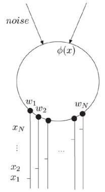
Figure 1: Schematic of the architecture. The postsynaptic cell receives inputs from $N$ presynaptic neurons, a repeated external input $\phi(x)$, and unspecified noisy inputs. Presynaptic neuron $i$ spikes at time $x_{i}$ in each period of $\phi$, and has synaptic weight $w_{i}$ onto the postsynaptic cell.

The framework for the neural dynamics is the spike response model Gerstner et al. (1993), without refractoriness.

Each presynaptic cell $i$ spikes exactly once at a fixed time within each sweep of the repeated external input, causing a corresponding postsynaptic potential response (PSP) in the postsynaptic cell.

The total membrane potential in the postsynaptic cell is the sum of these PSPs, weighted by synaptic efficacies (weights) $w_{i}$, and the two external inputs. This membrane potential induces the postsynaptic cell to spike at a certain (noisy) rate. Each presynaptic spike causes a constant (nonassociative) change in the weight $w_{i}$, and each postsynaptic and presynaptic spike pair causes a change in $w_{i}$ according to a spike-timing dependent learning rule, namely a function of the time difference between the postsynaptic and presynaptic spikes (associative learning).

The repeated external input is modeled as a periodic input with period T. We use two time variables: $x\in[0,T)$ for the time within each repetition of the external input, and $t=nT$, $n\in\mathbb{Z}$ for the time of initiation of each such period Roberts (1999); Roberts and Bell (2000); Roberts (2000b). General dynamical quantities will be functions of the pair $(x,t)$. Let $x_{i}$ be the time within each period when presynaptic cell $i$ spikes, and $w_{i}(x,t)$ its corresponding weight. Since presynaptic spikes are time-locked to the external input, $x_{i}$ is independent of $t$. Let $\mathcal{E}(s)$ be the PSP evoked by neuron $i$ at time $s$ after a spike. We assume $\mathcal{E}$ is causal: $\mathcal{E}(s)=0$ for $s<0$. Let $\alpha$ be the nonassociative weight change due to a presynaptic spike, and $\mathcal{L}(s)$ the associative weight change due to a postsynaptic spike time $s$ after a presynaptic spike. Let $\phi(x)$ be the periodic external input, and $U(x,t)$ the total postsynaptic potential due to the non-noisy inputs. We assume that for each $t$, the mean instantaneous postsynaptic spike rate density (in $x$) is given by $f(U(x,t))$ for some positive and strictly increasing function $f$. The function $f$ can be thought of as the effective gain of the postsynaptic cell in the presence of the noisy inputs. High or low noise correspond to an $f$ with small or large maximum slope respectively. No attempt is made to include a refractory period for postsynaptic spikes; and we will assume the period of $\phi$ is greater than the refractory period of the presynaptic neurons, so that refractoriness on the presynaptic side is irrelevant.

Changes in weights will be implemented as discrete steps with no internal time course. In the present model there are two natural choices for the time at which weight changes occur: asynchronously (instantaneously, whenever a presynaptic or postsynaptic spike occurs), or synchronously (once per sweep of the repeated external input, updating all weights simultaneously). We adopt the latter strategy, updating weights at $x=0$ for each $t=nT,n\in\mathbb{Z}$. The value of $w_{i}$ in the period beginning at $(0,t)$ is then independent of $x$, and will be denoted $w_{i}(t)$. For synchronous updating to be a reasonable approximation, we must assume that weight changes per cycle are small relative to the weights themselves (slow learning rate). Changes in weights due to different spikes or spike pairs are assumed to add linearly.

In biological systems, synaptic weights have bounded magnitude and do not change sign. Since the present paper is focused solely on the dynamics near equilibria, we impose no boundary conditions in the model. The results still apply to the biological case provided the weight equilibria are in the region enclosed by biological bounds.

We assume homogeneous parameters: the scalar $\alpha$ and the functions $\mathcal{E}$, $\mathcal{L}$ are the same for all presynaptic neurons, and the times $x_{i}$ are regularly spaced, $x_{i}=i\delta$, $i=0,1,\ldots,N-1$ for some $\delta>0$, $N=T/\delta\gg 1$.

For simplicity in the derivation of the weight dynamics, it will be convenient to assume that $\mathcal{E}(s),\mathcal{L}(s)$ are zero or negligible for $\lvert s\rvert>\tau_{E},\tau_{L}$ respectively, with $\tau_{E},\tau_{L}\ll T$. We will also require the learning rate to be slow: $T\ll\tau_{w}$, where $\tau_{w}$ is the time-scale on which weights undergo significant relative change. For the existence of approximate negative image states we will need the spacing of presynaptic spike times much smaller than the widths of $\mathcal{E}$ and $\mathcal{L}$: $\delta\ll\tau_{E},\tau_{L}$. These time-scale assumptions can be summarized as

$$\delta\ll(\tau_{E},\tau_{L})\ll T\ll\tau_{w}.$$

Typical values for the mormyrid ELL are: $\delta<1\text{ms}$ Bell et al. (1992), [C.C. Bell, private communication], $\tau_{E}\sim 20\text{ms}$ Bell et al. (1997a), $\tau_{L}\sim 40\text{ms}$ Bell et al. (1997a), $T\sim 80\text{ms}$ [C.C. Bell, private communication], $\tau_{w}\sim 10^{2}T$ Bell et al. (1997a).

III Weight Dynamics

To obtain the mean weight dynamics, we compute the mean value of $w_{i}(t+T)-w_{i}(t)$. The nonassociative change in $w_{i}(t)$ due to the single presynaptic spike at $(x_{i},t)$ is $\alpha$. For the associative change due to presynaptic and postsynaptic spike pairs, consider the effect of a single postsynaptic spike at $(x,t)$. The pairing of this spike with the presynaptic spike at $(x_{i},t)$ causes a change $\mathcal{L}(x-x_{i})$ in $w_{i}$. To properly handle edge effects, we also include the pairing with presynaptic spikes at $(x_{i},t-T)$ and $(x_{i},t+T)$, for a total change of

$$\mathcal{L}(x-x_{i}-T)+\mathcal{L}(x-x_{i})+\mathcal{L}(x-x_{i}+T).$$ (1)

For typical biological applications, where $\tau_{L}\ll T$, at most one of the above terms is non-negligible, but all must be included to handle cases where $x-x_{i}$ is within $\tau_{L}$ of $T$ or $-T$ (Fig. 2).

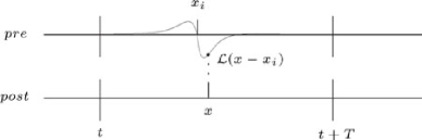
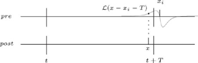
Figure 2: Changes in weight due to pairing of presynaptic and postsynaptic spikes. (a) Pairing of a postsynaptic spike at time $(x,t)$ and presynaptic spike by neuron $i$ at time $(x_{i},t)$ causes a change $\mathcal{L}(x-x_{i})$ in weight $w_{i}$. (b) For $x$ within $\tau_{L}$ of a period edge, we must include pairing with presynaptic spikes in the neighboring period. Pairing of a postsynaptic spike at time $(x,t)$ and presynaptic spike by neuron $i$ at time $(x_{i},t+T)$ cause a change $\mathcal{L}(x-x_{i}-T)$ in weight $w_{i}$.

In addition, $\tau_{L}\ll T$ allows us to approximate Eq. (1) by

$$\sum_{-\infty}^{\infty}\mathcal{L}(x-x_{i}-nT)=\overset{\circ}{\mathcal{L}}(x-x_{i}),$$ (2)

where $\overset{\circ}{\mathcal{L}}(s)=\sum_{-\infty}^{\infty}\mathcal{L}(s-nT)$ is the periodization of $\mathcal{L}$ with period $T$.

Quantity (2) is the change in $w_{i}(t)$ due to a single postsynaptic spike at $(x,t)$. Postsynaptic spikes between $t$ and $t+T$ occur at a mean rate density $f(U(x,t))$; hence the mean total change due to all postsynaptic spikes between $t$ and $t+T$ is

$$\int_{0}^{T}dx\,f(U(x,t))\overset{\circ}{\mathcal{L}}(x-x_{i}).$$

The mean total change in $w_{i}(t)$ due to both nonassociative and associative learning is therefore

$$\langle\triangle w_{i}(t)\rangle=\alpha+\int_{0}^{T}dx\,f(U(x,t))\overset{\circ}{\mathcal{L}}(x-x_{i}).$$ (3)

We now compute the postsynaptic potential $U(x,t)$. The contribution to $U(x,t)$ due to the presynaptic spike by neuron $i$ at $(x_{i},t-nT)$ is $w_{i}(t+nT)\mathcal{E}(x-x_{i}+nT)$. For $\tau_{E}\ll T$ this quantity is non-negligible for at most one value of $n$, either $n=0$ (current period) or $n=-1$ (previous period). But to properly handle edge effects (Fig. 3) we include both, for a total contribution of

$$w_{i}(t-T)\mathcal{E}(x-x_{i}-T)+w_{i}(t)\mathcal{E}(x-x_{i}).$$ (4)

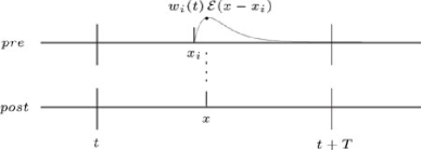
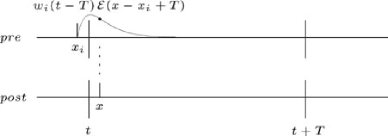
Figure 3: Postsynaptic potential due to presynaptic spikes. (a) Potential at time $(x,t)$ due to presynaptic spike by neuron $i$ at time $(x_{i},t)$ is $w_{i}(t)\mathcal{E}(x-x_{i})$. (b) For $x$ within $\tau_{E}$ of $0$, we must include the potential due to presynaptic spikes in the preceding period. The potential at time $(x,t)$ due to the presynaptic spike by neuron $i$ at time $(x_{i},t-T)$ is $w_{i}(t-T)\mathcal{E}(x-x_{i}+T)$.

We assume that the learning rate is sufficiently slow that we may approximate quantity (4) by

$$w_{i}(t)(\mathcal{E}(x-x_{i}-T)+\mathcal{E}(x-x_{i})).$$ (5)

Finally, $\tau_{E}\ll T$ allows us to approximate quantity (5) by

$$w_{i}(t)\sum_{-\infty}^{\infty}\mathcal{E}(x-x_{i}-nT)=w_{i}(t)\overset{\circ}{\mathcal{E}}(x-x_{i}),$$ (6)

where $\overset{\circ}{\mathcal{E}}(s)=\sum_{-\infty}^{\infty}\mathcal{E}(s-nT)$ is the periodization of $\mathcal{E}$ with period $T$.

Quantity (6) is the contribution to $U(x,t)$ from neuron $i$. The total postsynaptic potential is the summed contribution from all presynaptic neurons, plus the repeated external input:

$$U(x,t)=\phi(x)+\sum_{j=1}^{N}w_{j}(t)\overset{\circ}{\mathcal{E}}(x-x_{j})$$ (7)

Equations Eq. (3) and Eq. (7) define the mean weight dynamics. The common periodicity of the functions $\overset{\circ}{\mathcal{E}}$, $\overset{\circ}{\mathcal{L}}$ and $\phi$ is an important feature, allowing the systematic use of Fourier techniques.

IV The Negative Image

A set of weights $\{w_{i}\}$ for which the total postsynaptic potential $U(x,t)$ is approximately constant in $x$ will be referred to as an approximate negative image state. For such a state the contribution to the postsynaptic potential due to the presynaptic cells alone is, up to an additive constant $U_{0}$, an approximate negative image (Fig. 4) of the external input $\phi$:

$$\sum_{j=1}^{N}w_{j}\overset{\circ}{\mathcal{E}}(x-x_{j})\simeq U_{0}-\phi(x).$$ (8)

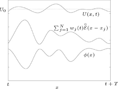
Figure 4: An approximate negative image. If the postsynaptic potential $U(x,t)=\phi(x)+\sum_{j=1}^{N}w_{j}(t)\overset{\circ}{\mathcal{E}}(x-x_{j})$ is approximately some constant $U_{0}$, then the potential $\sum_{j=1}^{N}w_{j}(t)\overset{\circ}{\mathcal{E}}(x-x_{j})$ due to presynaptic spikes alone is approximately $U_{0}-\phi(x)$.

In the following, we first show that approximate negative image states exist provided a certain condition holds on the Fourier coefficients of the postsynaptic potential function $\overset{\circ}{\mathcal{E}}$ and the repeated external input $\phi$, and provided the presynaptic spike time-spacing $\delta$ is sufficiently small. We then show that for a particular value of $U_{0}$ (depending on $\alpha$, $\overset{\circ}{\mathcal{L}}$, and $f$) there exists an approximate negative image state which is also an equilibrium (fixed point) for the weight dynamics.

For generic $\overset{\circ}{\mathcal{E}}$ and $\phi$, Eq. (8) cannot be made an exact equality for all $x$, because that would require solving infinitely many independent linear equations (one for each $x$) in only finitely many unknowns (the N weights $\{w_{j}\}$). But if we replace the discrete set of weights $w_{j}$ by a continuum weight density $\mathcal{W}$, then the analog of Eq. (8) can, under certain conditions, be made exact for all $x$. Given such a density, we then recover the biological case of discrete weights $\{w_{j}\}$ for which Eq. (8) is approximately true by defining the set $\{w_{j}\}$ to be a discrete approximation to $\mathcal{W}$.

Let $\mathcal{W}(y)$ be a weight density, with $\mathcal{W}(y)dy$ being the total weight for presynaptic spikes occurring between $y$ and $y+dy$, for $y\in[0,T)$. The continuum analog of Eq. (8), with exact equality for all $x$, is

$$\int_{0}^{T}dy\mathcal{W}(y)\overset{\circ}{\mathcal{E}}(x-y)=U_{0}-\phi(x).$$ (9)

To solve this equation for $\mathcal{W}$ we take the Fourier decomposition. Let $W_{n}=(1/T)\int_{0}^{T}dy\,e^{ik_{n}y}W(y)$ for $k_{n}=2\pi n/T$, $n\in\mathbb{Z}$ be the Fourier coefficients for $\mathcal{W}$, and let $E_{n}$, $\phi_{n}$ be the coefficients for $\overset{\circ}{\mathcal{E}}$ and $\phi$. Then Eq. (9) becomes

$$U_{0} - \sum_{n=-\infty}^{\infty}\phi_{n}e^{-ik_{n}x}$$

$$= \int_{0}^{T}dy(\sum_{n=-\infty}^{\infty}W_{n}e^{-ik_{n}y})(\sum_{m=-\infty}^{\infty}E_{m}e^{-ik_{m}(x-y)})$$

$$= \sum_{n=-\infty}^{\infty}\sum_{m=-\infty}^{\infty}W_{n}E_{m}e^{-ik_{m}x}\int_{0}^{T}dye^{i(k_{m}-k_{n})y}$$

$$= T\sum_{n=-\infty}^{\infty}W_{n}E_{n}e^{-ik_{n}x}.$$

Hence $\mathcal{W}$ satisfies Eq. (9) if and only if

$$W_{0} = \frac{U_{0}-\phi_{0}}{TE_{0}},$$

$$W_{n} = \frac{-\phi_{n}}{TE_{n}},\quad n\neq 0.$$ (10)

Given such a $\mathcal{W}$, we construct approximate negative image states with discrete weights as follows. Define $g(x)$ to be the deviation from a negative image:

$$g(x)=\phi(x)-U_{0}-\sum_{j=1}^{N}w_{j}\overset{\circ}{\mathcal{E}}(x-x_{j}).$$ (11)

Then $\{w_{j}\}$ is an approximate negative image state if $g(x)$ is small relative to $U_{0}-\phi(x)$, for all $x$. Consider the set of weights defined by

$$w_{j}=\delta\,\,\mathcal{W}(x_{j}),$$

where $\delta$ is the spacing of the $x_{j}$. These weights can be thought of as a discrete approximation to the weight density $\mathcal{W}(y)$. Substituting into Eq. (11) and using Eq. (9) gives

$$g(x) = \sum_{j=1}^{N}\delta\,\,\mathcal{W}(x_{j})\overset{\circ}{\mathcal{E}}(x-x_{j})-\int_{0}^{T}dy\mathcal{W}(y)\overset{\circ}{\mathcal{E}}(x-y).$$

This is the difference between a Riemann sum and the integral it approximates. The error theorem for Riemann sums then gives an upper bound for $g$:

$$\lvert g(x)\rvert\leq\delta\frac{T}{2}\max_{y}\lvert\frac{d}{dy}[\mathcal{W}(y)\overset{\circ}{\mathcal{E}}(x-y)]\rvert.$$ (12)

Hence, for $\lvert g(x)\rvert$ to be small, we need $\mathcal{W}(y)\overset{\circ}{\mathcal{E}}(x-y)$ to be differentiable in $y$, hence $\mathcal{W}(y)$ to be differentiable in $y$. A theorem of Fourier series Champeney (1987) says that $\mathcal{W}(y)$ is differentiable if $\sum_{n=-\infty}^{\infty}\lvert nW_{n}\rvert<\infty$. By Eq. (10) this places a constraint on the Fourier coefficients of $\overset{\circ}{\mathcal{E}}$ and $\phi$:

$$\sum_{n=-\infty}^{\infty}\lvert\frac{n\phi_{n}}{E_{n}}\rvert<\infty.$$ (13)

This inequality requires $\phi_{n}$ to go to zero as $n\to\pm\infty$ more rapidly than $E_{n}/n^{2}$. In particular, the high frequency (large $\lvert n\rvert$) spectral content of $\phi$ must be less than the high frequency content of $\overset{\circ}{\mathcal{E}}$. Intuitively, in order for the convolution of $\overset{\circ}{\mathcal{E}}$ with a smooth weight density $\mathcal{W}$ to be able to “match” the high frequency components of $-\phi$, the high frequency content of $\phi$ cannot be too large.

If Eq. (13) is satisfied, and $\delta$ is sufficiently small, then from Eq. (12) the deviation $g(x)$ from an exact negative image is small, hence approximate negative image states exist.

We now show that for a particular $U_{0}$ there exists an approximate negative image state that is an equilibrium for the weight dynamics. From Eq. (3), a weight state $\{w_{j}\}$ is an equilibrium if $U(x)=\phi(x)+\sum_{j=1}^{N}w_{j}\overset{\circ}{\mathcal{E}}(x-x_{j})$ satisfies

$$\alpha+\int_{0}^{T}dx\,f(U(x))\overset{\circ}{\mathcal{L}}(x-x_{i})=0\quad\text{for all}\,\,i.$$ (14)

This is a system of $N$ equations in the $N$ unknowns $\{w_{j}\}$, but they are nonlinear equations for nonlinear $f$. In general such equations need not have solutions, but for approximate negative image states the nonlinearity is in some sense “small”, and this will allow us to show that solutions exist provided $\delta$ is sufficiently small.

For an approximate negative image state we have $U(x)=U_{0}+g(x)$ with $g(x)\ll U_{0}$, and we wish this $U(x)$ to satisfy Eq. (14). First define $U_{0}$ so that Eq. (14) would be satisfied if $g(x)$ were identically zero:

$$\alpha+\int_{0}^{T}dx\,f(U_{0})\overset{\circ}{\mathcal{L}}(x-x_{i})=0\quad\text{for all}\,\,i.$$ (15)

This requires

$$f(U_{0}) = \frac{-\alpha}{\int_{0}^{T}dx\,\overset{\circ}{\mathcal{L}}(x-x_{i})}\quad\text{for all}\,i$$ (16)

$$= \frac{-\alpha}{\int_{0}^{T}dx\,\overset{\circ}{\mathcal{L}}(x)},$$

where the independence of $i$ follows from the periodicity of $\overset{\circ}{\mathcal{L}}$. Hence our desired $U_{0}$ exists and is given by

$$U_{0}=f^{-1}\Bigl{(}\frac{-\alpha}{\int_{0}^{T}dx\,\overset{\circ}{\mathcal{L}}(x)}\Bigr{)},$$ (17)

provided $\alpha$, $\overset{\circ}{\mathcal{L}}$ and $f$ satisfy

$$\min_{u}f(u)<\frac{-\alpha}{\int_{0}^{T}dx\,\overset{\circ}{\mathcal{L}}(x)}<\max_{u}f(u).$$ (18)

From Eq. (15), $U(x)=U_{0}+g(x)$ satisfies Eq. (14) if and only if

$$\int_{0}^{T}dx\,[f(U_{0}+g(x))-f(U_{0})]\overset{\circ}{\mathcal{L}}(x-x_{i})=0\quad\text{for all}\,\,i.$$ (19)

For brevity let $h(x)=f(U_{0}+g(x))-f(U_{0})$ and $L_{i}(x)=\overset{\circ}{\mathcal{L}}(x-x_{i})$. Then Eq. (19) can be written as

$$\langle h,L_{i}\rangle=0\quad\text{for all}\,\,i,$$ (20)

where $\langle\cdot,\cdot\rangle$ is the inner product defined by

$$\langle f_{1},f_{2}\rangle=\int_{0}^{T}dx\,f_{1}(x)f_{2}(x),$$ (21)

for $f_{1}$, $f_{2}$ in the space $X$ of smooth functions on the interval $[0,T]$.

Let $H$ be the set of functions $h$ corresponding to all possible values of the weights $\{w_{j}\}$:

$$H=\{h:h(x)=f(\phi(x)-\sum_{j=1}^{N}w_{j}\overset{\circ}{\mathcal{E}}(x-x_{j}))-f(U_{0}),$$

$$\,w_{j}\in\mathbb{R},\,j=1,\ldots,N\},$$

where we have used $U_{0}+g(x)=\phi(x)-\sum_{j=1}^{N}w_{j}\overset{\circ}{\mathcal{E}}(x-x_{j})$ from Eq. (11). Let $S$ be the subspace of $X$ consisting of all linear combinations of the $\{L_{i}\}$, and $S^{\bot}$ be the (infinite dimensional) subspace of $X$ orthogonal to $S$ (in the inner product defined by Eq. (21)). Then there exists an $h$ satisfying Eq. (20) if and only if $H$ and $S^{\bot}$ have nonempty intersection:

$$H\cap S^{\bot}\neq\emptyset.$$ (22)

We claim that condition (22) holds if $\delta$ is sufficiently small. If $\delta$ is small, then the bound (12) implies that $g(x)$ is small for all $x$. In that case $h(x)=f(U_{0}+g(x))-f(U_{0})$ is approximately its linearization in $g$, which we denote by $h_{0}(x)$:

$$h(x)\simeq h_{0}(x) = f^{\prime}(U_{0})g(x)$$

$$= f^{\prime}(U_{0})(\phi(x)-U_{0}+\sum_{j=1}^{N}w_{j}\overset{\circ}{\mathcal{E}}(x-x_{j})).$$

Let $H_{0}$ be the set of such $h_{0}$ corresponding to all possible values of the weights $\{w_{j}\}$:

$$H_{0}=\{h_{0}:h_{0}(x)=f^{\prime}(U_{0})(\phi(x)-U_{0}+\sum_{j=1}^{N}w_{j}\overset{\circ}{\mathcal{E}}(x-x_{j})),$$

$$\,w_{j}\in\mathbb{R},\,j=1,\ldots,N\},$$

Then the condition that $H_{0}$ have nonempty intersection with $S^{\bot}$,

$$H_{0}\cap S^{\bot}\neq\emptyset,$$ (23)

is equivalent to existence of $h_{0}\in H_{0}$ such that $\langle h_{0},L_{i}\rangle=0$ for all $i$. This is equivalent to the linearization of the system (19):

$$\int_{0}^{T}dx\,f^{\prime}(U_{0})(\phi(x)-U_{0}+\sum_{j=1}^{N}w_{j}\overset{\circ}{\mathcal{E}}(x-x_{j}))\overset{\circ}{\mathcal{L}}(x-x_{i})=0$$

$$\quad\text{for all}\,\,i,$$

which can be rewritten as

$$\sum_{j=1}^{N}Q_{ij}w_{j}=\gamma,$$ (24)

where $\gamma=\int_{0}^{T}dx\,f^{\prime}(U_{0})(\phi(x)-U_{0})$ and

$$Q_{ij}=f^{\prime}(U_{0})\int_{0}^{T}dx\,\overset{\circ}{\mathcal{E}}(x-x_{j})\overset{\circ}{\mathcal{L}}(x-x_{i}).$$ (25)

This is a system of $N$ linear inhomogeneous equations in the $N$ unknowns $\{w_{j}\}$, which has a solution provided the coefficient matrix $Q$ is invertible. The eigenvalues of $Q$ will be calculated in the following section, and for generic $\mathcal{E}$ and $\mathcal{L}$ all eigenvalues are nonzero. Hence $Q$ is generically invertible, so that condition (23) holds. Furthermore, the intersection of $H_{0}$ with $S^{\bot}$ is generically transversal (not tangent).

Now as $\delta\to 0$, $H\to H_{0}$ (in the metric induced by the inner product (21)). By the openness of transversal intersection (infinite dimensional version, Abraham and Robbin (1967)), any sufficiently small perturbation of $H_{0}$ also intersects $S^{\bot}$. Hence for $\delta$ sufficiently small, $H$ intersects $S^{\bot}$ (Fig. 5), hence $h$ satisfying Eq. (20) exists. The corresponding weight state $\{w_{j}\}$ is an approximate negative image equilibrium.

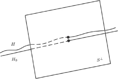
Figure 5: Transversal intersection theorem. If $H_{0}$ has transversal intersection with $S^{\bot}$ and $H$ is sufficiently close to $H_{0}$, then $H$ intersects $S^{\bot}$.

V Stability Criterion

We now derive a necessary and sufficient condition for the mean stability of approximate negative image equilibria, by examining the linearized weight dynamics around such states. Let $\{\hat{w}_{j}\}$ be an approximate negative image equilibrium satisfying Eq. (11) with

$$U(x)=\phi(x)+\sum_{j=1}^{N}\hat{w}_{j}\overset{\circ}{\mathcal{E}}(x-x_{j})=U_{0}+\hat{g}(x)$$ (26)

Solving for $\phi(x)$ in Eq. (26) and substituting into (7) yields

$$U(x,t) = U_{0}+\hat{g}(x)+\sum_{j=1}^{N}v_{j}(t)\overset{\circ}{\mathcal{E}}(x-x_{j}),$$

where $v_{j}(t)=w_{j}(t)-\hat{w}_{j}$ is the deviation of weight $j$ from its equilibrium value, and $\hat{g}(x)$ is the deviation from a negative image in the equilibrium state $\{\hat{w}_{j}\}$. To first order in $v_{j}$ we then have

$$f(U(x,t))\simeq f(U_{0}+\hat{g}(x))+f^{\prime}(U_{0}+\hat{g}(x))\sum_{j=1}^{N}v_{j}(t)\overset{\circ}{\mathcal{E}}(x-x_{j}).$$ (27)

Substituting Eq. (27) into Eq. (3) and using $\triangle w_{i}(t)=\triangle v_{i}(t)$ yields

$$\langle\triangle v_{i}(t)\rangle=\alpha+\int_{0}^{T}dx\,f(U_{0}+\hat{g}(x))\overset{\circ}{\mathcal{L}}(x-x_{i})$$

$$+f^{\prime}(U_{0}+\hat{g}(x))\sum_{j=1}^{N}v_{j}(t)\overset{\circ}{\mathcal{E}}(x-x_{j}))\overset{\circ}{\mathcal{L}}(x-x_{i}).$$

From the equilibrium condition Eq. (14) and Eq. (26), the term in Eq. (V) of zeroth order in $v_{j}$ vanishes. Hence

$$\langle\triangle v_{i}(t)\rangle\simeq\sum_{j=1}^{N}P_{ij}v_{j}(t),$$

where

$$P_{ij}=\int_{0}^{T}dx\,f^{\prime}(U_{0}+\hat{g}(x))\overset{\circ}{\mathcal{E}}(x-x_{j}))\overset{\circ}{\mathcal{L}}(x-x_{i}).$$

Now assume $\delta$ is sufficiently small that

$$\hat{g}(x)\ll\frac{f^{\prime}(U_{0})}{f^{\prime\prime}(U_{0})}\quad\text{for all }x.$$

Then $f^{\prime}(U_{0}+\hat{g}(x))\simeq f^{\prime}(U_{0})$ for all $x$, so that $P_{ij}\simeq Q_{ij}$, where $Q$ is the matrix defined in Eq. (25), and we obtain

$$\langle\triangle v_{i}(t)\rangle\simeq\sum_{j=1}^{N}Q_{ij}v_{j}(t).$$

Taking the mean on both sides and using $\langle\triangle v_{i}(t)\rangle=\triangle\langle v_{i}(t)\rangle$ yields

$$\triangle\langle v_{i}(t)\rangle\simeq\sum_{j=1}^{N}Q_{ij}\langle v_{i}(t)\rangle.$$ (28)

Eq. (28) gives the linearized dynamics for $\langle v_{i}(t)\rangle$ near $\langle v_{i}(t)\rangle=0$, hence for $\langle w_{i}(t)\rangle$ near the approximate negative image equilibrium $\{\hat{w}_{j}\}$.

The system Eq. (28) is stable if and only if all eigenvalues of $Q+I$ have norm less than 1. Due to periodicity of $\overset{\circ}{\mathcal{E}},\overset{\circ}{\mathcal{L}}$ and regular spacing of the $\{x_{i}\}$, the matrix $Q$ has the property that each of its rows equals the row above it shifted one entry to the right (and wrapped around at the edges). Such matrices are called circulant Davis (1979) and their eigenvectors and eigenvalues are easily found, as follows. Let $u$ be the vector with components $u_{i}=e^{ikx_{i}}$; then

$$(Qu)_{i} = \sum_{j=1}^{N}Q_{ij}u_{j}$$

$$= \sum_{j=1}^{N}e^{ikx_{j}}\int_{0}^{T}dx\,\overset{\circ}{\mathcal{E}}(x-x_{j})\overset{\circ}{\mathcal{L}}(x-x_{i}),$$

so that

$$\frac{(Qu)_{i}}{u_{i}}=\sum_{j=1}^{N}e^{ik(x_{j}-x_{i})}\int_{0}^{T}dx\,\overset{\circ}{\mathcal{E}}(x-x_{j})\overset{\circ}{\mathcal{L}}(x-x_{i}).$$ (29)

By periodicity of $\overset{\circ}{\mathcal{E}}$ and $\overset{\circ}{\mathcal{L}}$, the integral in the above expression is a function of $x_{j}-x_{i}$ modulo $T$. The factor $e^{ik(x_{j}-x_{i})}$ is also a function of $x_{j}-x_{i}$ modulo $T$ provided $e^{ikT}=1$. Now if the $\{x_{i}\}$ are regularly spaced, the sum over $j$ of a function of $x_{j}-x_{i}$ modulo $T$ is independent of $i$. In that case Eq. (29) would imply $(Qu)_{i}/u_{i}$ independent of $i$, hence $u$ is an eigenvector of $Q$, with eigenvalue the right hand side of Eq. (29). We get a complete set of such eigenvectors by taking $N$ values of $k$ such that $e^{ikT}=1$ and the functions $e^{ikx_{i}}$ are independent functions of $i$. Here we choose

$$k_{n}=\frac{2\pi n}{T},\quad n=0,1,...,N-1.$$

The corresponding eigevalues of $Q$ are

$$\lambda_{n} = \sum_{j=1}^{N}e^{ik_{n}(x_{j}-x_{i})}\int_{0}^{T}dx\,\overset{\circ}{\mathcal{E}}(x-x_{j})\overset{\circ}{\mathcal{L}}(x-x_{i}).$$

Letting $z_{j}=x_{j}-x_{i}$, making the change of variables $y=x_{j}-x$ and using periodicity of $\overset{\circ}{\mathcal{E}}$, $\overset{\circ}{\mathcal{L}}$ gives

$$\lambda_{n} = \sum_{j=1}^{N}e^{ik_{n}z_{j}}\int_{0}^{T}dy\overset{\circ}{\mathcal{E}}(-y)\overset{\circ}{\mathcal{L}}(z_{j}-y)$$

$$= \sum_{j=1}^{N}e^{ik_{n}x_{j}}\overset{\circ}{\mathcal{L}}*_{T}\widetilde{\overset{\circ}{\mathcal{E}}}\,(x_{j}),$$

where $*_{T}$ is convolution on the interval $[0,T]$, $\widetilde{\,\,}$ is horizontal reflection ($\widetilde{\overset{\circ}{\mathcal{E}}}(y)=\overset{\circ}{\mathcal{E}}(-y))$, and since $\{z_{j}\}=\{x_{j}\}$ we have replaced $z_{j}$ by $x_{j}$ in the sum.

The stability condition is $\lvert 1+\lambda_{n}\rvert<1$ for all $n$:

Stability:

$$\lvert 1+\sum_{j=1}^{N}e^{ik_{n}x_{j}}\overset{\circ}{\mathcal{L}}*_{T}\widetilde{\overset{\circ}{\mathcal{E}}}\,(x_{j})\rvert<1,$$ (30)

$$\quad k_{n}=\frac{2\pi n}{T},\,n=0,1,...,N-1.$$

In the biological setting two limiting regimes are of special interest: slow learning ($\overset{\circ}{\mathcal{L}}$ small) and dense spacing ($\delta$ small).

If $\overset{\circ}{\mathcal{L}}$ is small, then so are the eigenvalues of $Q$. If $\lambda_{n}=a_{n}+ib_{n}$ with $a_{n},b_{n}$ real, we have

$$\lvert 1+\lambda_{n}\rvert^{2}=(1+a_{n})^{2}-b_{n}^{2}=1+2a_{n}+(a_{n}^{2}-b_{n}^{2}).$$

If $a_{n}$ and $b_{n}$ are sufficiently small, this quantity is less than $1$ if and only if $a_{n}<0$. Hence for $\overset{\circ}{\mathcal{L}}$ sufficiently small, all eigenvalues of $Q+I$ have norm less than $1$ if and only if all eigenvalues of $Q$ have negative real part. The stability condition then becomes $Re\,\lambda_{n}<0$ for all $n$. Hence in the slow learning limit Eq. (30) becomes

Slow learning:

$$Re\sum_{j=1}^{N}e^{ik_{n}x_{j}}\overset{\circ}{\mathcal{L}}*_{T}\widetilde{\overset{\circ}{\mathcal{E}}}\,(x_{j})<0,\quad n=0,1,...,N-1.$$ (31)

The dense spacing limit ($\delta\to 0$) is the continuum limit in $x_{i}$. The discrete weight density $w_{i}/T$ is replaced by a continuum weight density $W(x)$, sums over $x_{j}$ are replaced by integrals over $x$, and $N\to\infty$. This yields

$$\lambda_{n} = \int_{0}^{T}dx\,e^{ik_{n}x}\overset{\circ}{\mathcal{L}}*_{T}\widetilde{\overset{\circ}{\mathcal{E}}}\,(x)\quad n=0,1,...$$

Hence $\lambda_{n}$ is just the $n^{th}$ Fourier coefficient of $\overset{\circ}{\mathcal{L}}*_{T}\widetilde{\overset{\circ}{\mathcal{E}}}$. The Fourier convolution theorem then gives

$$\lambda_{n}=\overset{\circ}{L}_{n}\widetilde{\overset{\circ}{E}}_{n}=\overset{\circ}{L}_{n}\overline{\overset{\circ}{E}_{n}},$$

where $\overset{\circ}{E}_{n},\widetilde{\overset{\circ}{E}}_{n},\overset{\circ}{L}_{n}$ are the $n^{th}$ Fourier coefficients of $\overset{\circ}{E},\widetilde{\overset{\circ}{E}},\overset{\circ}{L}$ respectively, and $\overline{z}$ is the complex conjugate of $z$. Substituting into the stability condition $\lvert 1+\lambda_{n}\rvert<1$ for all $n$ gives the dense spacing limit of Eq. (30):

Dense spacing:

$$\lvert 1+\overset{\circ}{L}_{n}\overline{\overset{\circ}{E}_{n}}\rvert<1,\quad n=0,1,...$$ (32)

Finally, with both slow learning and dense spacing the stability condition becomes

Slow learning, dense spacing:

$$Re[\overset{\circ}{L}_{n}\overline{\overset{\circ}{E}_{n}}]<0,n=0,1,...$$ (33)

A further simplification follows in the long period limit, $\tau_{E},\tau_{L}\ll T$. Holding $\tau_{E},\tau_{L}$ constant and taking $T\to\infty$, the Fourier series of $\overset{\circ}{\mathcal{E}},\overset{\circ}{\mathcal{L}}$ in Eq. (33) approach Fourier transforms of $\mathcal{E},\mathcal{L}$. The stability condition then becomes

Slow learning, dense spacing, long period:

$$Re[\mathcal{F}\left[\mathcal{L}\right](k)\overline{\mathcal{F}\left[\mathcal{E}\right]}(k)]<0,\quad k\in(-\infty,\infty).$$ (34)

For the calculation of examples we will work in the slow learning, dense spacing, long period limit, which is the limit of primary biological interest in the mormyrid ELL.

VI General Remarks

The Roles of Nonassociative and Associative Learning. Both nonassociative and associative learning ($\alpha$ and $\mathcal{L}$, respectively) play a role in whether approximate negative image equilibria exist, via Eq. (18). They are also both involved in determining the location of such equilibria, via Eq. (14). The interpretation of Eq. (14) is that at equilibrium, the mean change due to nonassociative learning ($\alpha$) must be precisely opposite to the mean change due to associative learning (the $\mathcal{L}$ term). If the postsynaptic spike rate density $f$ is bounded, this places a relative magnitude constraint on $\alpha$ and $\mathcal{L}$, namely Eq. (18). If this constraint is violated then the mean changes due to associative and nonassociative learning are unable to balance one another, and no negative image equilibrium is possible.

By contrast, only associative learning plays a role in the stability of approximate negative image equilibria, via Eq. (30). The irrelevance of nonassociative learning for stability has an intuitive interpretation: near an approximate negative image equilibrium, the mean nonassociative change is cancelled by the mean associative change due the constant postsynaptic potential $U_{0}$ around which $U(x,t)$ fluctuates. Only the deviations of $U(x,t)$ from $U_{0}$ cause a net change in the weights, and these changes are purely associative (due to postsynaptic spikes generated by $U(x,t)$). Alternatively, nonassociative learning can be analogized to a constant externally applied force in a physical system. Such a force changes the location of equilibria, but has no effect on the dynamics around equilibria.

The Role of the Repeated Input. For a given postsynaptic potential response $\mathcal{E}$, the repeated input $\phi$ plays a role in the existence of approximate negative image states via Eq. (13): $\phi$ cannot have too much high frequency content relative to $\mathcal{E}$ for such states to exist.

Assuming $\phi$ is such that approximate negative image states exist, it then plays the important role of determining the weight configurations in such states, an in particular in approximate negative image equilibria, via Eq. (8).

But $\phi$ plays no role in the stability of the resulting negative image equilibrium. This is intuitively reasonable, since in approximate negative image states $\phi$ is “nulled out” by the summed postsynaptic potentials due to time-locked presynaptic spikes.

The Role of Noise. The functional form of the mean postsynaptic spike rate $f$ affects the existence and location of the negative image equilbrium via Eq. (18) and Eq. (14).

But provided $f$ is strictly increasing (so that $f^{\prime}$ is positive), $f$ has no effect on the stability of the equilibrium. Hence the classification of learning rules as (mean) stable or unstable is, except for this mild monotonicity requirement, insensitive to the fine structure of the noise. This is a post hoc justification for not modeling the noise in more detail.

Canonically Stable Learning Rule: $\mathcal{L}=-\mathcal{E}$. In the dense spacing and slow learning limit, suppose $\mathcal{L}=-\mathcal{E}$. The stability condition Eq. (33) is then

$$\lvert\overset{\circ}{E}_{n}\rvert^{2}>0\qquad\text{for all}\,\,n,$$ (35)

or in other words, $\overset{\circ}{E}_{n}\neq 0$ for all $n$. Since this is true for generic $\mathcal{E}$, the learning rule $\mathcal{L}=-\mathcal{E}$ is generically stable.

Area Sign Condition. In the dense spacing and slow learning limit, consider $n=0$ in Eq. (33). Since $\overset{\circ}{L}_{0}$ and $\overline{\overset{\circ}{E}_{0}}=\overset{\circ}{E}_{0}$ are just the areas under the functions $\overset{\circ}{\mathcal{L}}$ and $\overset{\circ}{\mathcal{E}}$, Eq. (33) says that for stability, these areas must be opposite in sign. If they are the same sign, then the negative image is unstable. In particular, if $\mathcal{E}$ and $\mathcal{L}$ are both nonnegative, the negative image is unstable. Hence, if $\mathcal{E}$ is an excitatory PSP and $\mathcal{L}$ is any pure potentiating learning rule, the negative image is unstable. Similarly, inhibitory PSPs with purely depressing learning rules are unstable.

Symmetric and Antisymmetric Learning Rules. In the dense spacing, slow learning, long period limit, there is a nonempty, positive measure set of postsynaptic response functions for which purely symmetric or purely antisymmetric learning rules are generically unstable. This follows from the fact that the Fourier transforms of symmetric and antisymmetric functions are pure real and pure imaginary, respectively.

Suppose the real part of the Fourier transform of $\mathcal{E}$ has a zero:

$$Re[\mathcal{F}\left[\mathcal{E}\right](k_{0})]=0,\quad\text{for some }k_{0}.$$ (36)

Then, generically, $Re[\mathcal{F}\left[\mathcal{E}\right](k)]$ changes sign at $k_{0}$. Suppose $\mathcal{L}$ is symmetric, so that $\mathcal{F}\left[\mathcal{L}\right](k)$ is pure real. Then

$$Re[\mathcal{F}\left[\mathcal{L}\right](k)\overline{\mathcal{F}\left[\mathcal{E}\right]}(k)]=\mathcal{F}\left[\mathcal{L}\right](k)\,Re[\mathcal{F}\left[\mathcal{E}\right](k)].$$

Since $Re[\mathcal{F}\left[\mathcal{E}\right](k)]$ changes sign at $k_{0}$, for the stability condition Eq. (34) to be satisfied for $k$ near $k_{0}$, we must have $\mathcal{F}\left[\mathcal{L}\right](k)$ change sign at $k_{0}$, in the opposite sense to $Re[\mathcal{F}\left[\mathcal{E}\right](k)]$; see Fig. 6. But this forces $\mathcal{F}\left[\mathcal{L}\right](k_{0})=0$, which is untrue for generic symmetric $\mathcal{L}$. Hence generic symmetric learning rules are unstable for postsynaptic response functions satisfying Eq. (36).

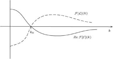
Figure 6: If $Re[\mathcal{F}\left[\mathcal{E}\right](k)]$ changes sign at $k_{0}$, then for the product $\mathcal{F}\left[\mathcal{L}\right](k)Re[\mathcal{F}\left[\mathcal{E}\right](k)]$ to be negative around $k_{0}$ we must have $\mathcal{F}\left[\mathcal{L}\right](k)$ also change sign at $k_{0}$, in the opposite sense to $Re[\mathcal{F}\left[\mathcal{E}\right]](k)$.

Similarly, if the imaginary part of the Fourier transform of $\mathcal{E}$ has a zero:

$$Im[\mathcal{F}\left[\mathcal{E}\right](k_{0})]=0,\quad\text{for some }k_{0}.$$ (37)

then generic antisymmetric learning rules are unstable.

Pure antisymmetric learning rules have another difficulty: since they satisfy $\int_{0}^{T}dx\,\mathcal{L}(x)=0$, near a negative image equilibrium the mean weight change per cycle due to an antisymmetric $\mathcal{L}$ is zero, to first order in $g$. The total mean weight change per cycle is therefore approximately $\alpha$. Hence negative image equilibria for pure antisymmetric learning rules are only possible if $\alpha=0$ (no nonassociative learning).

Cooperative Stability. It follows from Eq. (30) that the sum of stable learning rules is stable; but it is also clear that given a generic $\mathcal{E}$, there exist pairs of learning rules $\mathcal{L}_{1}$ and $\mathcal{L}_{2}$, each individually unstable, for which the sum $\mathcal{L}_{1}+\mathcal{L}_{2}$ is stable. This is most easily seen by direct computation in the slow learning, dense spacing, long period limit, via Eq. (34) (see the examples calculated below).

Duality Principle. Interchanging $\mathcal{L}$ and $\mathcal{E}$ in Eq. (25) transforms $Q_{ij}$ to $Q_{ji}$, hence $Q$ to $Q^{T}$, hence $Q+I$ to $(Q+I)^{T}$. The eigenvalues of a matrix are unchanged by transposition. The stability condition, that all eigenvalues of $Q+I$ have norm less than $1$, is thus invariant under interchange of $\mathcal{L}$ and $\mathcal{E}$. In other words, a PSP $\mathcal{E}$ and learning rule $\mathcal{L}$ are a stable pair if and only if the PSP $\mathcal{L}$ and learning rule $\mathcal{E}$ are a stable pair.

This has potential biological relevance if the functional forms of PSPs and associative learning rules overlap. The single-lobe exponential and alpha function learning rules treated in the examples, below, are also plausible PSPs, hence duality applies.

Inversion Principle. Replacing $\mathcal{E}$ by $-\mathcal{E}$ and $\mathcal{L}$ by $-\mathcal{L}$ in Eq. (25) leaves $Q_{ij}$ invariant, hence $Q+I$ invariant. The stability condition is therefore invariant under inversion of both $\mathcal{E}$ and $\mathcal{L}$. In other words, a PSP $\mathcal{E}$ and learning rule $\mathcal{L}$ are a stable pair if and only if the PSP $-\mathcal{E}$ and learning rule $-\mathcal{L}$ are a stable pair.

In particular, the stable learning rules for an inhibitory PSP are just minus the stable learning rules for the corresponding excitatory PSP. Plasticity at inhibitory synapses was explored in Roberts (2000c), and preliminary experimental evidence given in Han et al. (1999).

Independence of Normalization. In the slow learning and dense spacing limit, the stability conditions Eq. (33) or Eq. (34) are invariant under multiplication of $\mathcal{L}$ or $\mathcal{E}$ by positive constants. Hence, provided the magnitudes of $\mathcal{L}$ or $\mathcal{E}$ are not so large that the slow learning assumption is violated, stability does not depend on those magnitudes. In particular, in working with specific examples it is not necessary to give $\mathcal{L}$ or $\mathcal{E}$ any overall normalization.

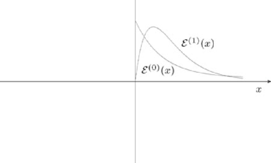
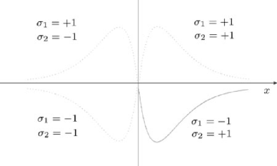
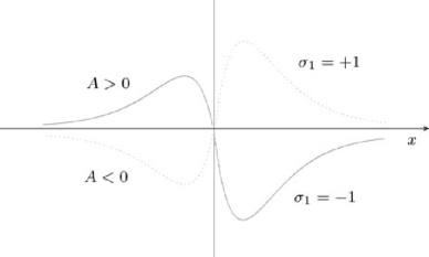
Figure 7: PSPs and learning rules used in the examples. (a) The PSP $\mathcal{E}^{(p_{E})}(x)$ is exponential for $p_{E}=0$ and an alpha function for $p_{E}=1$. (b) One-lobe learning rules of alpha function form, $\mathcal{L}_{I}^{(1)}(x)$, for the four possible combinations of $\sigma_{1}$ (potentiating or depressing) and $\sigma_{2}$ (pre-before-post or post-before-pre). (c) Two-lobe learning rules of alpha function form, $\mathcal{L}_{II}^{(1)}(x)$, for the four possible combinations of $\sigma_{1}$ (pre-before-post lobe potentiating or depressing) and the sign of $A$ (post-before-pre lobe potentiating or depressing). The area of the pre-before-post lobe is normalized to $\pm 1$, and the area of the post-before-pre lobe is $A$.

VII Examples

Working in the slow learning, dense spacing, long period limit, we now compute explicit criteria for stability when $\mathcal{E}$ and $\mathcal{L}$ have functional forms commonly used in the spike-timing dependent plasticity literature. The PSP $\mathcal{E}$ will be assumed excitatory and causal, and of exponential or alpha function form. The learning rule $\mathcal{L}$ will consist of one or two “lobes”: a “pre-before-post” lobe (presynaptic spike before postsynaptic spike) and/or a “post-before-pre” lobe (postsynaptic spike before presynaptic spike). Each lobe will be of exponential or alpha function form, and either potentiating (positive) or depressing (negative). Such $\mathcal{E}$ and $\mathcal{L}$ can be written as follows:

$$\mathcal{E}^{(p_{E})}(x) =x^{p_{E}}e^{-x/\tau_{E}}H(x)$$

$$\mathcal{L}_{I}^{(p_{L})}(x) =\sigma_{1}\,(\sigma_{2}x)^{p_{L}}e^{-\sigma_{2}x/\tau_{L}}H(\sigma_{2}x)$$ (one-lobe)

$$\mathcal{L}_{II}^{(p_{L})}(x) =\frac{\sigma_{1}}{\tau_{L_{1}}^{p_{L}+1}}\,x^{p_{L}}e^{-x/\tau_{L_{1}}}H(x)$$

$$\quad+\frac{A}{\tau_{L_{2}}^{p_{L}+1}}\,(-x)^{p_{L}}e^{x/\tau_{L_{2}}}H(-x)$$ (two-lobe)

where $H$ is the Heaviside function

$$H(x)=\begin{cases}1&x\geq 0,\\ 0&x<0.\end{cases}$$

The parameters (see Fig. 7) are as follows: $p_{E},p_{L}=0$ for an exponential or $1$ for an alpha function; $\tau_{E}$, $\tau_{L}$, $\tau_{L_{1}}$ and $\tau_{L_{2}}$ are positive time constants; $\sigma_{1}=+1$ for a potentiating lobe or $-1$ for a depressing lobe; $\sigma_{2}=+1$ for a pre-before-post lobe or $-1$ for a post-before-pre lobe; and for the two-lobe $\mathcal{L}$, $A$ is the area of the post-before-pre lobe, with the area of the pre-before-post lobe normalized to $\pm 1$ . We impose no overall normalization on $\mathcal{E}$ or $\mathcal{L}$, since this has no effect on stability.

We assume an excitatory PSP $\mathcal{E}$; to obtain the stable cases for the inhibitory PSP $-\mathcal{E}$, simply replace $\mathcal{L}$ by $-\mathcal{L}$ in the stable cases for $\mathcal{E}$ (i.e. replace $\sigma_{1}$ by $-\sigma_{1}$ and $A$ by $-A$).

For both the one-lobe and two-lobe $\mathcal{L}$, there are four possible combinations of $p_{E}$ and $p_{L}$: exponential or alpha function PSP with exponential or alpha function learning rule. We will refer to these four cases as ee, ea, ae, and aa, with the first letter in the pair indicating that the PSP is exponential or alpha function, and the second letter referring to the learning rule.

The Fourier transforms of these $\mathcal{E}$ and $\mathcal{L}$ are rational functions in $k$, and the stability condition will reduce to the requirement that a certain polynomial in $k^{2}$, whose coefficients are themselves polynomials in the parameters of $\mathcal{E}$ and $\mathcal{L}$, be negative for all $k$. Since the algebra in all cases is essentially the same, differing only in the size and coefficients of the resulting polynomial, we present only one case (aa, one-lobe) in full detail and for all other cases simply list the end results.

VII.1 Alpha Function PSP, One-Lobe Alpha Function Learning Rule

For

$$\mathcal{E}(x) = xe^{-x/\tau_{E}}H(x)$$

$$\mathcal{L}(x) = \sigma_{1}\sigma_{2}xe^{-\sigma_{2}x/\tau_{L}}H(\sigma_{2}x)$$

we have

$$\mathcal{F}\left[\mathcal{E}\right](k) = \frac{\tau_{E}^{2}}{(1-ikE)^{2}}$$

$$\mathcal{F}\left[\mathcal{L}\right](k) = \frac{\sigma_{1}\tau_{L}^{2}}{(1-\sigma_{2}ik\tau_{L})^{2}}$$

leading to

$$Re\Big{\{}\mathcal{F}\left[\mathcal{L}\right](k)\overline{\mathcal{F}\left[\mathcal{E}\right]}(k)\Big{\}}$$

$$= C\,Re[\sigma_{1}(1+i\sigma_{2}k\tau_{L})^{2}(1-ik\tau_{E})^{2}]$$

$$= C\sigma_{1}[\sigma_{2}^{2}\tau_{L}^{2}\tau_{E}^{2}k^{4}+(4\sigma_{2}\tau_{L}\tau_{E}-\sigma_{2}^{2}\tau_{L}^{2}-\tau_{E}^{2})k^{2}+1]$$

where $C=\tau_{L}^{2}\tau_{E}^{2}/[(1+\sigma_{2}^{2}\tau_{L}^{2}k^{2})^{2}(1+\tau_{E}^{2}k^{2})^{2}]$. Since $C>0$, the stability condition is then

$$\sigma_{1}[\sigma_{2}^{2}r^{2}k^{4}+(4\sigma_{2}r-\sigma_{2}^{2}r^{2}-1)k^{2}+1]<0$$

$$\quad\text{for all}\,\,k$$ (38)

where $r=\tau_{L}/\tau_{E}$. The expression on the left is a quadratic in $k^{2}$. The condition is impossible for $\sigma_{1}=+1$ (it fails at $k=0$) but for $\sigma_{1}=-1$ more work is required. The quadratic $ax^{2}+bx+c$ is negative for all $x\geq 0$ if and only if $a<0$ and ($b<0$ or $b^{2}-4ac<0$). Applying this condition to Eq. (VII.1) with $\sigma_{1}=-1$ yields

$$r^{2}-4\sigma_{2}r+1 < 0$$ (39)

$$\text{or}\quad(r-\sigma_{2})^{2}(r^{2}-6\sigma_{2}r+1) < 0$$ (40)

For $\sigma_{2}=-1$ these give $-2-\sqrt{3}<r<-2+\sqrt{3}$ or $-3-2\sqrt{2}<r<-3+2\sqrt{2}$, both of which are impossible because $r>0$. For $\sigma_{2}=+1$ we get $2-\sqrt{3}<r<2+\sqrt{3}$ or $3-2\sqrt{2}<r<3+2\sqrt{2}$; the former is contained in the latter, giving stability if and only if

$$\sigma_{1}=-1,\sigma_{2}=+1,$$

$$3-2\sqrt{2}<\frac{\tau_{L}}{\tau_{E}}<3+2\sqrt{2}.$$ (41)

The only stable case is depressive and pre-before-post, with $\tau_{L}/\tau_{E}$ constrained to lie in a finite interval (Fig. 8). Note that this interval contains $\tau_{L}/\tau_{E}=1$, where $\mathcal{L}=-\mathcal{E}$ (the canonically stable learning rule).

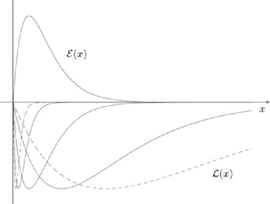
Figure 8: Range of stable one-lobe $\mathcal{L}$ for given $\mathcal{E}$, in case aa. The learning rule must be depressive and pre-before-post, with $3-2\sqrt{2}<\tau_{L}/\tau_{E}<3+2\sqrt{2}$. Stable examples are drawn with solid lines; endpoints of the stable interval are drawn with dashed lines.

Duality is also applicable here. Interchanging $\mathcal{E}$ and $\mathcal{L}$ in this example is equivalent to interchanging $\tau_{E}$ and $\tau_{L}$ and multiplying both $\mathcal{E}$ and $\mathcal{L}$ by $-1$. The multiplications offset and we are left with $r$ replaced by $1/r$. It follows that if the interval of stability for the pair $(\mathcal{E},\mathcal{L})$ is $s_{1}<r<s_{2}$, the corresponding interval for the pair $(\mathcal{L},\mathcal{E})$ is $s_{1}<1/r<s_{2}$. But by duality these intervals must coincide; hence we must have $s_{1}=1/s_{2}$. This is indeed the case for $s_{1}=3-2\sqrt{2}$ and $s_{2}=3+2\sqrt{2}$.

The instability of the $\sigma_{1}=+1$ case for any $\tau_{E}$ and $\tau_{L}$, by the failure of the stability condition at $k=0$, is just the Area Sign Condition.

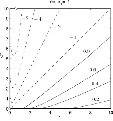
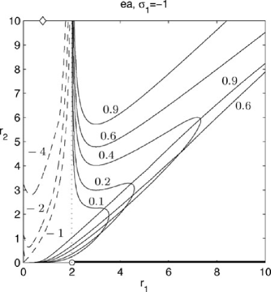
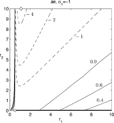
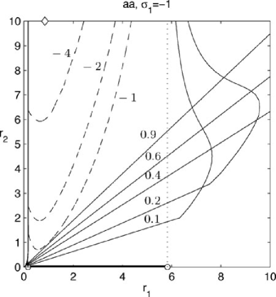
Figure 9: Boundary curves of the stable region in $(r_{1},r_{2})$ for various values of $A$, for two-lobe $\mathcal{L}$ with $\sigma_{1}=-1$. Curves are labelled by $A$. Curves with $A>0$ are drawn with solid lines, curves with $A<0$ with dashed lines. In all cases the region of stability is on the side of the curve containing the diamond ($\diamond$) in the upper left corner of the plot. The interval of stability for the corresponding one-lobe learning rules is the portion of the $r_{1}$-axis in bold.

VII.2 Summary of Results

For the one-lobe learning rules the stable parameter ranges are all easily calculated:

ee:

$\sigma_{1}=-1,\sigma_{2}=+1$:  all $\tau_{L}/\tau_{E}$

ea:

$\sigma_{1}=-1,\sigma_{2}=+1$:  $\tau_{L}/\tau_{E}<2$

ae:

$\sigma_{1}=-1,\sigma_{2}=+1$:  $\tau_{L}/\tau_{E}>1/2$

aa:

$\sigma_{1}=-1,\sigma_{2}=+1$: $2-\sqrt{3}<\tau_{L}/\tau_{E}<2+\sqrt{3}.$

Note that in all four cases we get instability, for all $\tau_{L}$ and $\tau_{E}$, if $\mathcal{L}$ is not depressive and pre-before-post. For $\mathcal{L}$ depressive and pre-before-post, all four cases have some range of $\tau_{L}/\tau_{E}$ in which $\mathcal{L}$ is stable. The extent of that range depends critically on the precise functional form of $\mathcal{E}$ and $\mathcal{L}$; but for $1/2<\tau_{L}/\tau_{E}<2$ we have stability independent of the functional form of $\mathcal{E}$ and $\mathcal{L}$.

For the two-lobe learning rules the polynomial arising out of the stability condition has coefficients depending on $\sigma_{1}$ and on three continuous parameters: $r_{1}$, $r_{2}$ and $A$, where $r_{1}=\tau_{L_{1}}/\tau_{E}$, $r_{2}=\tau_{L_{2}}/\tau_{E}$. The polynomials are given in the Appendix.

In all four cases, $\sigma_{1}=+1$ is always unstable. For $\sigma_{1}=-1$, the boundaries of the stable region in $(r_{1},r_{2})$ for various values of $A$ are plotted numerically in Fig. 9.

For one-lobe learning rules we found that only depressive and pre-before-post permits stability. For two-lobe learning rules, the pre-before-post lobe must be depressive for stability, and the post-before-pre lobe cannot have area $A$ greater than 1. This is just the Area Sign Condition: the area of the pre-before-post lobe is -1, and for stability when paired with an excitatory PSP $\mathcal{E}$ the total area under the learning rule $\mathcal{L}$ must be negative.

For $A<1$, the effect of the post-before-pre lobe shows the following general trends: in cases ee and ae, as the absolute area $\lvert A\rvert$ of the post-before-pre lobe increases, the stable region in the relative time constants $r_{1}$ and $r_{2}$ tends to shrink. Hence the post-before-pre lobe can be thought of as destabilizing in such cases. In cases ee and ae the situation is less clear. Increasingly negative $A$ (larger depressive post-before-pre) is uniformly destabilizing, but increasingly positive $A$ (larger potentiating post-before-pre) appears to be destabilizing for small $r_{2}$ but stabilizing for large $r_{2}$.

Cooperative stability, in which a two-lobe rule is stable while each of its lobes individually would be unstable, occurs in cases ea, ae, and aa: any point $(r_{1},r_{2})$ in a stable region, with $r_{1}$ outside the interval in which the corresponding one-lobe rule is stable is an example of cooperative stability.

Finally, the shape and extent of stable regions for two-lobe learning rules, or the extent of stable intervals for one-lobe learning rules, depend critically on whether $\mathcal{E}$ and $\mathcal{L}$ are exponential or alpha function in form. This suggests that in order to infer even such qualitative properties as stability or instability in a biological context, the learning rule must be known with considerable precision.

However, for particular values of some parameters the dependence on functional form may be such that useful conclusions can still be drawn in the absence of such precision; for example, the stability in one-lobe, depressive pre-before-post learning rules with $\tau_{L}/\tau_{E}\simeq 1$, independent of whether $\mathcal{E}$ or $\mathcal{L}$ are exponential or alpha function in form. This particular finding has direct relevance to the learning rule observed experimentally in mormyrid ELL Bell et al. (1997a). The experimental data is not precise enough to suggest a particular functional form, but does indicate a one-lobe, depressive, pre-before-post rule, with a width of the same order of magnitude as the width of a PSP. Stability of such a rule is consistent with the analytic results derived above.

VIII Appendix

For completeness we provide below the polynomial conditions for stability of the two-lobe learning rules treated in the examples.

ee:

$ak^{4}+bk^{2}+c<0\quad\text{for all}\,\,k$
 $a=\sigma_{1}r_{1}r_{2}^{2}-Ar_{1}^{2}r_{2}$
 $b=\sigma_{1}(r_{2}^{2}+r_{1})+A(r_{1}^{2}-r_{2})$
 $c=\sigma_{1}+A$

ea:

$ak^{6}+bk^{4}+ck^{2}+d<0\quad\text{for all}\,\,k$
 $a=\sigma_{1}r_{1}r_{2}^{3}(2r_{2}-1)-Ar_{1}^{3}r_{2}(2r_{1}+1)$
 $b=\sigma_{1}r_{2}(r_{2}^{3}-3r_{1}^{2}r_{2}+6r_{1}r_{2}+r_{1})+Ar_{1}(r_{1}^{3}-3r_{1}r_{2}^{2}-6r_{1}r_{2}+r_{2})$
 $c=\sigma_{1}(2r_{2}^{2}-r_{1}^{2}+2r_{1})+A(2r_{1}^{2}-r_{2}^{2}-2r_{2})$
 $d=\sigma_{1}+A$

ae:

$ak^{4}+bk^{2}+c<0\quad\text{for all}\,\,k$
 $a=\sigma_{1}r_{2}^{2}(2r_{1}-1)-Ar_{1}^{2}(2r_{2}+1)$
 $b=\sigma_{1}(r_{2}^{2}+2r_{1}-1)+A(r_{1}^{2}-2r_{2}-1)$
 $c=\sigma_{1}+A$

aa:

$ak^{8}+bk^{6}+ck^{4}+dk^{2}+e<0\quad\text{for all}\,\,k$
 $a=\sigma_{1}r_{1}^{2}r_{2}^{4}+Ar_{1}^{4}r_{2}^{2}$
 $b=\sigma_{1}(-r_{2}^{4}-2r_{1}^{2}r_{2}^{3}+4r_{1}r_{2}^{4}-r_{1}r_{2}^{3}+3r_{1}^{2}r_{2}^{2}+2r_{1}r_{2}^{2})\\ +Ar_{1}(-r_{1}^{4}+2r_{1}^{3}r_{2}^{2}-4r_{1}^{4}r_{2}-r_{1}^{3}r_{2}=2r_{1}^{2}r_{2}+3r_{1}^{2}r_{2}^{2})$
 $c=\sigma_{1}(-3r_{1}r_{2}+(r_{1}^{2}+r_{2}^{2})(r_{2}+1)^{2}+r_{2}^{2}(1+4r_{1}-4r_{1}r_{2}))\\ +A(-3r_{1}r_{2}+(r_{1}^{2}+r_{2}^{2})(r_{1}-1)^{2}+r_{1}^{2}(1-4r_{2}-4r_{1}r_{2}))$
 $d=\sigma_{1}(2r_{2}^{2}-r_{1}^{2}+4r_{1}-1)+A(2r_{1}^{2}-r_{2}^{2}-4r_{2}-1)$
 $e=\sigma_{1}+A$