Long-range Static Directional Stress Transfer
in a Cracked, Nonlinear Elastic Crust

Abstract

Seeing the Earth crust as crisscrossed by faults filled with fluid at close to lithostatic pressures, we develop a model in which its elastic modulii are different in net tension versus compression. In constrast with standard nonlinear effects, this “threshold nonlinearity” is non-perturbative and occurs for infinitesimal perturbations around the lithostatic pressure taken as the reference. For a given earthquake source, such nonlinear elasticity is shown to (i) rotate, widen or narrow the different lobes of stress transfer, (ii) to modify the $1/r^{2}$ 2D-decay of elastic stress Green functions into the generalized power law $1/r^{\gamma}$ where $\gamma$ depends on the azimuth and on the amplitude of the modulii asymmetry. Using reasonable estimates, this implies an enhancement of the range of interaction between earthquakes by a factor up to $5-10$ at distances of several tens of rupture length. This may explain certain long-range earthquake triggering and hydrological anomalies in wells and suggest to revisit the standard stress transfer calculations which use linear elasticity. We also show that the standard double-couple of forces representing an earthquake source leads to an opening of the corresponding fault plane, which suggests a mechanism for the non-zero isotropic component of the seismic moment tensor observed for some events.

1 Introduction

There are many evidences that faults and earthquakes interact, as suggested by calculations of stress redistribution [1], elastodynamic propagation of ruptures using laboratory-based friction law [2, 4], simplified models of multiple faults [5, 6], as well as general constraints of kinematic and geometric compatibility of the deformations [7]. Maybe the simplest mechanism for earthquake interaction involves stress re-distribution, both static [8, 1] and dynamical [9] associated with a given earthquake modeled as a set of dislocations or cracks. In this simple mechanical view, earthquakes cast stress shadows in lobes of stress unloading [10, 8] and increase the probability of rupture in zones of stress increase [11], according to the laws of linear elasticity. These elastic stress transfer models are useful for their conceptual simplicity and are increasingly used. Notwithstanding their extended use, the calculations of stress transfer have large uncertainties stemming from (i) the usually poorly known geometry of the rupture surfaces, (ii) the unconstrained homogeneity and amplitude of the stress drop and/or of the slip distribution on the fault plane, (iii) the use of simplified models of the crust (3D semi-infinite, or thin elastic plate, or plate coupled to a semi-infinite visco-elastic asthenosphere, etc.), and (iv) the unknown direction and amplitude of the absolute stress field that pre-existed before the event, including its possible spatial inhomogeneity.

Such elastic stress transfer models seem unable to account for a growing phenomenology of long-range earthquake interactions. For instance, many large earthquakes have been preceded by an increase in the number of intermediate sized events over very broad areas [12, 13]. The relation between these intermediate sized events and the subsequent main event has only recently been recognized on a large scale because the precursory events occur over such a large area that they do not fit prior definitions of foreshocks [14]. In particular, the $11$ earthquakes in California with magnitudes greater than $6.8$ in the last century are associated with an increase of precursory intermediate magnitude earthquakes measured in a running time window of five years [15]. What is strange about the result is that the precursory pattern occured with distances of the order of $300$ to $500~{}km$ from the futur epicenter, i.e. at distances up to ten times larger that the size of the futur earthquake rupture. Furthermore, the increased intermediate magnitude activity switched off rapidly after a big earthquake in about half of the cases. This implies that stress changes due to an earthquake of rupture dimension as small as $35~{}km$ can influence the stress distribution to distances more than ten times its size. These observations of earthquake-earthquake interactions over long times and large spatial separations have been strengthened by several other works on different catalogs using a variety of techniques [13, 16]. These results defy usual mechanical models of linear elasticity and one proposed explanation is that seismic cycles represent the approach to and retreat from a critical state of a fault network [16, 17]. Within the critical earthquake concept, the anomalous long-range interactions between earthquakes reflect the increasing stress-stress correlation length upon the approach of the critical earthquake. Another explanation involves dynamical stress triggering [18] (see however [19]). Additional seismic, geophysical, and hydrogeological observations [20] cannot be accounted for by using models derived from the elastic stress transfer mechanism. In particular, standard poro-elastic models underestimate grossly the observed amplitudes of hydrogeological anomalous rises and drops in wells at large distances from earthquakes.

2 Mechanical Model of the Earth’s Crust

Here, we investigate the hypothesis, and its implications for the above observations, that the crust is a nonlinear elastic medium characterized by an asymmetric response to compressive versus extensive perturbations around the lithostatic stress. We call this a “threshold nonlinearity.” This nonlinearity stems from a mechanically-justified argumentation based on the fact that the Earth’s crust at seismogenic depth is crisscrossed by joints, cracks or faults at many different scales filled with drained fluid in contact with delocalized reservoirs at pressures close to the lithostatic pressure. It has been argued that rock permeability and thus microcracking adjusts itself, so that fluid pressure is always close to rock pressure irrespective of the extend of hydration/dehydration [21, 23]. One possible mechanism for this involves a time-dependent process that relates fluid pressure, flow pathways and fluid volumes [24].

2.1 Presence and role of fluids

Indeed, a lot of data collectively support the existence of significant fluid circulation to crustal depths of at least $10-15km$. Much attention has been devoted to the role of overpressurized fluid [25, 26, 27, 28, 29, 30]. It is more and more recognized that fluids play an essential role in virtually all crustal processes. Ref.[31] reviews the historical development of the conciousness among researchers of the ubiquitous presence and importance of fluids within the crust. Numerous examples exist that demonstrate water as an active agent of the mechanical, chemical [32] and thermal processes that control many geologic processes that operate within the crust [21, 22]. The bulk of available information on the behavior of fluids comes from observations of exposed rocks that once resided at deeper crustal levels. In any case, present day surface exposed metamorphic rocks indicate that, at all crustal levels, fluids have been present in significant volume. Because the porosity of metamorphic rock is probably less than $1\%$, the high volume of calculated fluid necessary to produce observed chemical changes suggests that fluid must have been replenished thousands of times. It has also been proposed that gold-quartz vein fields in metamorphic terranes provide evidence for the involvement of large volumes of fluids during faulting and may be the product of seismic processes [33]. Water is also released from transformed minerals. For instance, Montmorillonite changes to illite with a release of free water from the clay structure at approximately the same depth as the first occurrence of the anomalous pore pressure [34]. This is the most commonly discussed example of hydration and dehydration of minerals changing the fluid mass and the pore pressure. Fluids have been directly sampled at about $11~{}km$ by the Soviets at the Kola Peninsula drillhole.

Many observations suggest that there are massive crustal fluid displacements correlated with seismic events. Among them, one can cite the fault-valve mechanism [35] or the migration and diffusion of aftershocks [36]. Several mechanisms have been proposed for the mechanical effect of fluids to decrease compressive lithostatic stresses: mantle-derived source of fluids can maintain overpressure within a leaky fault [27]; laboratory sliding experiments on granite show that the sliding resistance of shear planes can be significantly decreased by pore sealing and compaction which prevent the communication of fluids between the porous deforming shear zone and the surrounding material [28]. Physico-chemical processes such as mineral dehydration during metamorphism may provide large fluid abundance over large areas [37, 22]. Such fluid presence or migration implies that cracks may open and close even at seismogenic depth, justifying the relevance of asymetric nonlinear elasticity for such depths as we elaborate below.

2.2 Physical mechanism for the threshold nonlinearity

From a mechanical point of view, the threshold nonlinearity we invoke is different from the ubiquitous nonlinearity of rocks. In the later, nonlinearity becomes important only under large deformations. Such nonlinear elasticity of rocks is well-documented from its nonlinear wave signatures [39]. In contrast, the nonlinearity we invoke is revealed for almost arbitrary small perturbations by the difference between compressive versus extensive perturbations around a mean lithostatic stress field. Many crustal rocks have a Young’s modulus depending on confining pressure, in particular with a Young’s modulus in tension smaller than the Young’s modulus in compression in a ratio from $1/2$ to $1/10$ [38].

The highly damaged upper crust, as described above, would behave as a standard continuous elastic medium if almost all cracks are kept closed and are thus completely transparent to the applied tectonic stress. In a totally dry crust, this would occur at depths larger than about $1km$. Near the surface, cracks can open under sufficiently tensile stresses, so that the rock (if we neglect crack growth phenomena) will display low elastic modulii (what we will call later a soft state). Under compressive (or weakly tensile) stresses, those same cracks will close so that the rock will display elastic modulii close to those of uncracked material (the hard state). This simple compressive/tensile asymmetry changes strongly the behaviour of the rock: the rheology is still elastic (in the sense that it is reversible) but it is nonlinear (a change of sign of applied stress does not only changes the sign of strain, it also changes its modulus). In addition, if we now take account of the possible slow growth of cracks under tensile stress, the nature of the nonlinearity will not change, but its amplitude will.

Let us now consider the influence of fluids whose presence are pervasive in the crust, as summarized in section 2.1. Let us assume that the crust is saturated with fluids and that the network of cracks is sufficiently dense so that it behaves as a drained medium. For the sake of simplicity, we will also assume that the crust is characterized by a homogeneous spatial distribution of cracks, so that the permeability is uniform and isotropic. We will also suppose that there exists a horizontal interface at depth $z_{seal}$ where permeability is $0$. The last ingredient is that the part of the crust below $z_{\rm seal}$ is connected to a reservoir of fluid. Many indirect observations suggest indeed the presence of large sources of fluids [40, 41]. Then, above depth $z_{\rm seal}$, water will be at hydrostatic pressure $P_{h}$ (lower than lithostatic pressure $P_{l}$) so that cracks will be able to close if the tensile applied tectonic stress is smaller than $P_{l}-P_{h}$ in modulus (cracks remain closed if tectonic stress is compressive). Below $z_{\rm seal}$, the scenario is different. Water trapped in cracks is now at lithostatic pressure. If there is no applied tectonic stress, fluid pressure inside cracks compensates exactly the lithostatic pressure and the medium is exactly at the hard/soft boundary. The net stress acting on any crack’s lips is $0$, so that the crack doesn’t grow. If the applied tectonic stress is compressive, cracks will close and fluids are expelled towards the reservoir: the crust is in the hard phase. If the applied tectonic stress is tensile, cracks will open and the crust is in the soft phase. If a crack becomes unstable, pressure drops within it, so that it tends to close to re-establish initial fluid pressure. If a crack grows very slowly, pressure within the crack will stay constant with time. We will from now on neglect the possible slow crack growths and assume that fluid pressure is constant in each crack and that the crack network geometry does not show any evolution with time or applied stress. Thus, below $z_{\rm seal}$, the applied stress threshold to get from the hard to the soft state is $0$. This explains our terminology of a “threshold nonlinearity.”

The remaining of the paper will investigate stress redistributions associated with earthquakes occurring below $z_{\rm seal}$. The existence of $z_{\rm seal}$ is difficult to prove for the real crust. It would correspond, for instance, to a depth where the crack network geometry changes abruptly, for instance at the boundary between the sedimentary basin and cristalline rocks. We can also propose an alternate model in which the vertical permeability below $z_{\rm seal}$ is much lower than the horizontal one, and would obtain the same kind of soft/hard transition. Note that much more complicated scenarii involving the chemistry of both fluids and rock matrix could be taken into account [22], but we choosed to neglect them in this purely mechanical paper.

We then propose a simple central-force spring model in two dimensions to study the behaviour of such an asymmetric nonlinear medium when subjected to an infinitesimal internal source of stress or strain. We show that the spatial structure of the stress transfer associated with such a perturbation evolves with the strength of the nonlinearity (defined as the ratio of the springs’ stiffness in tensile and in compressive states). Those changes are quantified in terms of the symmetry of the resulting stress field and of the decay rate of the amplitude of the stress perturbation with distance from the source.

3 Numerical Model

Solving theoretical problems of nonlinear elasticity proves to be very tough, even for the simple asymmetry of our threshold nonlinearity. We thus choosed to solve a couple of simple problems related to seismology using numerical modelling. Stress, strain and material rigidity being $2^{nd}$ or $4{th}$ rank tensors, and as there is an obvious and complex feedback between strain and rigidity in our model, we choosed to use a simple spring model to illustrate the concept and major consequences of the threshold nonlinear elasticity.

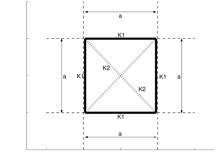
Figure 1: Mechanical structure of an elementary cell of the model. Each cell is defined by $4$ nodes linked by springs along edges and both diagonals. Springs on the edges are of stiffness $K_{1}$, while diagonal springs are of stiffness $K_{2}=K_{1}/2$ (see text).

A plate of size $L$ by $L$ is discretized onto a regular grid of mesh size $a$. In the following, we choose $L=2000km$ and $a=10km$. Each elementary cell is defined by $4$ nodes, each node being shared between $4$ different neighbouring cells (except on the boundary of the plate). Figure 1 shows the mechanical structure defined for each cell: each node is connected to its two nearest neighbours by springs of stiffness $K_{1}$ (those springs indeed define the $4$ edges of the cell). As those are central force springs, the shear modulus of such a cell is indeed $0$. To get shear elasticity [42], $2$ springs are added along the cell’s diagonals, such that each node is also connected to its next-nearest neighbours. The stiffness of those diagonal springs is $K_{2}$. Once the plate is discretized with such cells, it can be shown that the plate behaves as an isotropic elastic medium if and only if we have $K_{2}=K_{1}/2$ [44]. The two independent elastic modulii of the plate can then be shown to be $\lambda=\mu=K_{1}/2$ for the two Lamé coefficients, thus yielding $E=(4/3)K_{1}=(8/3)\mu$ for the Young modulus and $\nu=1/3$ for the Poisson coefficient (note that we are dealing with a pure $2D$ model). Of course, many other geometries of the elementary cell are possible, but we had to choose square cells which help to handle more easily with boundary conditions used in the problems we want to study.

The relationships we just defined are true only if the springs are symmetric, i.e., their stiffnesses is the same under tensile or compressive states. The next and last step to model our nonlinear threshold elastic rheology is to impose that the stiffness of each spring can vary with its length. Thus, if a spring is shortened, its stiffness will be, say, $K$. If a spring is lengthened, its stiffness is lower and taken equal to $\alpha K$, with $\alpha\leq 1$. Each spring represents an effective volume filled with a uniform and isotropic distribution of cracks with sizes smaller than the representative mesh size. Real damage in the crust is of course much more complex, with anisotropic, space and scale dependence. These complications are neglected in our first exploration. We can obtain an order of magnitude estimate of the density of fluid-filled faults associated with a given asymmetric coefficient $\alpha$, using the effective medium calculations in [43]. To simplify, let us assume $\lambda=\mu$. Then, $\alpha=\lambda_{d}/\lambda_{1}=1/(1+5d/2)$, where $\lambda_{d}$ is the Lamé coefficient of the damaged material and $d=N(\ell/L)^{3}$ is the density of faults (assumed identical) of radius $\ell$ in a cube of volume $L^{3}$. $N$ is the number of faults in that volume. For instance, we need about $11$ faults of size $L/3$ to get $\alpha=0.5$. Such estimate must however be taken with caution since the effective medium calculation $\alpha=1/(1+5d/2)$ is valid only for small crack densities, while any piece of rock and the real crust are crisscrossed by many faults at many length scales, most of them being healed at varying degrees. We think that values of $\alpha$ significantly smaller than $1$ should thus not be excluded. It is also probably that $\alpha$ is not uniform within the crust and can be expected to reflect the past history of deformations and ruptures.

The ratio $\alpha$ of the extensive over compressive elastic coefficient can also be seen as equivalent to $1-D_{m}$ in damage mechanics, where $D_{m}$ is the scalar damage variable. If the spring isn’t damaged, then $D=0$, so that $\alpha=1$ and the stiffness is the same under tensile and compressive states. If the spring is totally damaged (near failure), $D_{m}$ is close to $1$, so that $\alpha\simeq 0$ and the stiffness of the spring in tensile state vanishes, while it is still $K$ if the spring is compressed. Under arbitrary loading conditions, some springs in the plate will be in tensile state, while others will be in compressive state, so that it is difficult to analytically compute the stiffness tensor of the whole plate when $\alpha<1$. In addition, the stiffness tensor may feature more than $2$ independent modulii. This justifies the use of an iterative numerical method as described in the next section.

4 Numerical Method

The method we use belongs to the so-called iterative ‘type-writer’ methods. The first step consists in defining boundary conditions, i.e. to fix displacements and/or applied forces on set of nodes. As we are dealing with statics, such forces and displacements are held constants throughout the numerical process. We then consider, say, the node on the top left corner of the mesh and, according to the forces/displacements applied to this node and his nearest and next-nearest neighbours, we can compute the net force acting on that node. As we are dealing with a statics problem, the net force acting on that node at equilibrium should vanish. If the force vector we computed for that node is not $\overrightarrow{0}$, then we move it in the direction of the force vector to decrease the net force. We store the new position of this node and get to its right neighbour and follow the same scheme. We thus sweep the mesh line by line down to the node on the bottom right, and iterate the same operations again from the node on top left. As iterations accumulate, the net force acting on each node decreases, and we stop the process once all nodes are subjected to a force whose modulus is under a given threshold. This threshold is chosen such that the modulus of the incremental displacement necessary to decrease the net force modulus on each node is of the order of the accuracy of the computer, namely about $10^{-12}$. To avoid any spurious result due to the direction of type-writing, iterations alternatively begin on each of the four corners of the plate on either horizontal or vertical directions, right or left, up or down. Once the ‘type-writer’ is stopped, displacements of all nodes relative to their initial positions are stored. Those positions also allow to compute, for a given node, the forces exerted on it by each of its neighbours. Those last quantities allow to compute the full stress tensor at that node [44], which is also stored. Computations of forces transmitted by a spring from one node to another take account of the spring stiffness which, as described in the previous section, depends on the state (stretched or shortened) of the spring through the value of $\alpha$ which is kept constant throughout the network.

Starting from given boundary conditions, we solve a statics problem, which means that we do not take account of neither wave propagation nor fluid migration. We just compute the final equilibrium solution. This point will be discussed at the end of the paper when considering the application of this model to real Earth data.

5 Earthquake Modeling

In this paper, we want to examine the main differences between the stress field pattern generated by an earthquake in our nonlinear threshold elastic medium and in a standard linear elastic medium. The first step is thus to define mesh parameters representative of the real crust, the second one is to define what is an earthquake source in such a model.

5.1 Parametering the Earth’s crust

Our numerical model is strictly a $2D$ one, as dealing with the third dimension would lead to serious memory and computing time problems, and we would have to handle boundary problems such as the free surface and coupling with lower viscous layers. We can however choose mesh parameters such that, using relationships linking plane elasticity to $3D$ elasticity, we can model realistic crust properties (however neglecting boundary problems). The size of the plate as well of the cells has been previously given. We fixed the (virtual) thickness of the plate to be $10km$, so that it corresponds roughly to the thickness of the seismogenic zone within the crust. We then choosed $K_{c}=5\cdot 10^{14}~{}Nm^{-1}$ (where $K_{c}$ is the value of $K_{1}$ when springs are compressed), so that the $3D$ elastic modulii become $E=6.25\cdot 10^{10}~{}Pa$, $\lambda=\mu=2.5\cdot 10^{10}~{}Pa$, and $\nu=0.25$, which are close to usual modulii measured in rock mechanics experiments. The value of the assymmetry parameter $\alpha$ will be varied through several numerical experiments from $1$ (standard isotropic elasticity) down to $0.01$ (strong asymmetry of the elastic response under extension versus compression).

5.2 Earthquake Source modelling

Earthquake source theory has until now been theoretically studied within the framework of linear elasticity. This allows one to use very powerful tools such as the representation theorem and Green functions. An earthquake can then be viewed equivalently as a displacement discontinuity across a fault plane, or a distribution of double-couples and dipoles of forces along the same plane in a continuous medium [3, 45, 46].

In the case of a fault of finite dimensions, if we assume that the stress drop is uniform along the fault, then we deal with a crack problem. If we assume that the displacement discontinuity across the fault is uniform, then we deal with a dislocation problem. At distances from the fault much larger than its size, and in the case of linear elasticity, both models yield the same spatial patterns of stress and displacement fields, which are linked by Hooke’s law. This will be illustrated below in our diagrams obtained for the symmetric elasticity case $\alpha=0$.

In the nonlinear case, it is easy to show that the representation theorem fails to apply, and then so does the Green function concept. This stems from the fact that the principle of linear superposition fails in the presence of nonlinearity. It follows that even the most simple earthquake source problem has to be defined either as a crack or a dislocation problem, and both problems should give different stress and displacement patterns at long wavelengths. We will, in this preliminary work, study only pointwise sources, which will allow simple comparisons with elementary solutions obtained from linear elasticity.

We will thus study two cases:

• an initially stress-free medium within which a single cell (located at its center) is subjected to the following stress field tensor: $\sigma_{xx}=\sigma_{yy}=0$ while $\sigma_{xy}\not=0$ (and is hereafter called pointwise shear stress load or crack model) - this model is reminiscent of the standard dynamical model of an event in standard linear elasticity [3],

• an initially stress-free medium within which a single cell is subjected to a pure shear strain field: $\epsilon_{xx}=\epsilon_{yy}=0$ while $\epsilon_{xy}\not=0$ (hereafter called pointwise shear strain load or dislocation problem) - this model rather views the event as a shear displacement discontinuity.

In both cases, the corresponding infinitesimal planar defect (the source of the earthquake) suffers from undeterminacy and is oriented either along the $\vec{O}_{x}$ direction (plane $P_{x}$) or along the $\vec{O}_{y}$ direction (plane $P_{y}$). In the first case, the slip discontinuity is dextral, and it is sinistral in the second case.

5.3 Quantitative source parameters

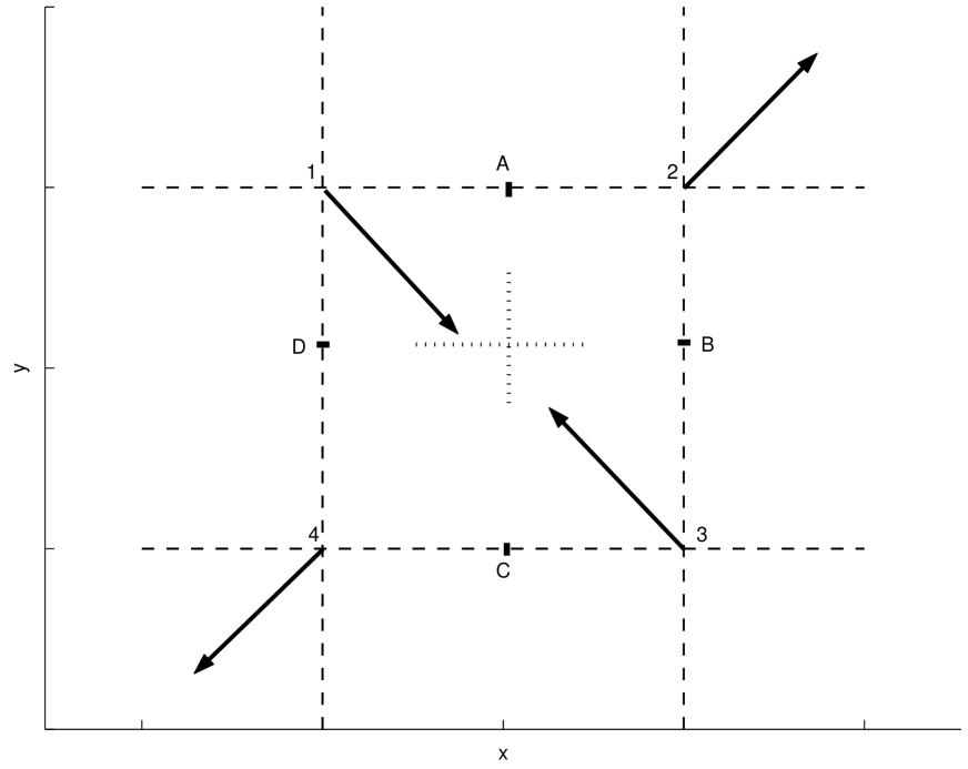
Figure 2: Representation of the elementary source in a unit cell. Vectors represent either forces of equal modulii (crack model) or displacement of same amplitude (dislocation model). Nodes of the cell are labelled $1,2,3,4$. Dotted lines represent the virtual plane defect along which force or displacement discontinuities are imposed to model an earthquake. Those discontinuities have to be computed at points labelled $A,B,C,D$ (see text).

The small scale of our mechanical model is that of a cell, and this is thus the smallest scale we have to deal with in order to model an earthquake source. Figure 2 shows the source cell and $4$ different vectors originating from each of its $4$ corners.

In the case of the pure shear stress load model, each vector represents a force applied to the corresponding node. All forces have the same modulus so that the stress tensor within the central cell indeed corresponds to the one we defined above. The same set of forces is applied whatever the value of $\alpha$.

In the case of the pure shear strain load model, each vector represents a displacement applied to the corresponding node. All displacements have the same modulus so that the strain tensor within the central cell indeed corresponds to the one we defined above. The same set of displacements is applied whatever the value of $\alpha$.

In order to ensure that we can compare results obtained from both types of boundary conditions, we have to fullfil a very simple condition: the stress and displacement fields must be identical in the classic linear case, i.e. when $\alpha=1$. In the pure shear stress load model, we imposed the modulus of each applied force equal to $F=7.1\cdot 10^{14}N$, so that is corresponds to an event of scalar moment $M_{0}=7.1\cdot 10^{18}~{}Nm$, i.e., of magnitude $\approx 6.5$. We computed the displacement field for $\alpha=1$, and observed that the magnitude of the displacement at each node of the source cell was $0.526640588m$. To be perfectly consistent, we thus impose this displacement amplitude at each source cell node in the case of the pure shear strain load model.

6 Displacement field at the source

In the pointwise dislocation case, displacements are held constant at the source whatever the value of $\alpha$. In the pointwise crack model, only forces are kept constant as $\alpha$ is changed, and displacements are expected to vary as the asymmetry increases (i.e. $\alpha$ decreases). We have already pointed out that both boundary conditions assume that the mechanical defect is either parallel to $P_{x}$ or to $P_{y}$. Indeed, we will show that the displacement (hereafter named $u_{n}$) normal to each of these conjugate defects is of the same type (opening) while the shear displacement (hereafter $u_{s}$) along each of them is of different type: dextral along $P_{x}$ and sinistral along $P_{y}$. That said, we will focus only on the modulii of those displacements.

How do we obtain $u_{n}$ and $u_{s}$? Indeed, according to the orientations of the conjugate plane defects, we have to compute displacements at points $A,B,C$ or $D$, whereas our model provides solutions at nodes $1,2,3$ and $4$ (see Figure 2). Displacements at points $A$ to $D$ are thus computed through bilinear interpolations within the cell. We then define $u_{n}=u_{x}(B)=-u_{x}(D)=-u_{y}(C)=u_{y}(A)$ and $u_{s}=u_{x}(A)=u_{y}(B)=-u_{x}(C)=-u_{y}(D)$ as a result of the symmetries of the system.

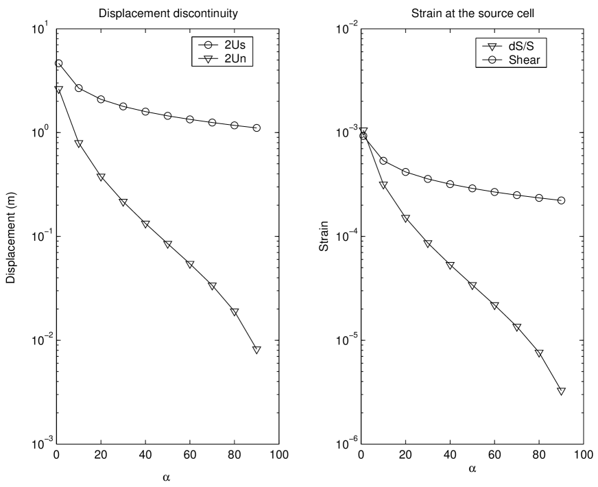
Figure 3: Left panel: shear (circles) and normal (triangles) displacements discontinuities along planar defects within the source cell as a function of $\alpha$ in semilogscale. Results for $\alpha=0$ are not shown as the normal discontinuity vanishes. Right panel: volumetric (circles) and shear (triangles) strains of the source cell as a function of $\alpha$ in semilogscale ($\alpha$ is the ratio of the elastic modulus in extension over the elastic modulus in compression). Results for $\alpha=0$ are not shown as the volumetric strain vanishes in this case. All results are obtained for the pure shear stress loading case.

Figure 3 shows the variations of both $u_{n}$ and $u_{s}$ with $\alpha$ (in fact, it shows the values of displacements discontinuities across the crack, i.e. $2u_{n}$ and $2u_{s}$). For $\alpha=1$, we find that $u_{n}$ is very close to $0$, so that the displacement along the pointwise crack lips is pure shear. As $\alpha$ decreases from $1$ to close to $0$, the shear displacements increase by a factor of about $4.5$. This is perfectly understandable, as some springs are sollicited in tension, leading to a decrease in their stiffness. This decrease, in the presence of constant forces, implies that displacements increase.

More surprising is the behaviour of normal displacements, which increase drastically as $\alpha$ decreases, tending to be about $2.7m$ when $\alpha$ tends to $0$ (i.e. about half the shear displacements). For $\alpha=0.1$ we have $u_{n}/u_{s}$ close to $1/3$. Moreover, $u_{n}$ and $u_{s}$ are both positive, which signifies that, under the shear stress load assumption, the defect opens when the medium is asymmetric. In seismological words, this means that the static moment tensor of the source has a non-vanishing trace and can thus be decomposed into an isotropic part and a deviatoric one. Despite the observation that most earthquake sources are thought to be well modelled by the deviatoric part alone, a few catalogues report isotropic components. Several mechanisms have been invoked to explain a non-vanishing isotropic component of the seismic moment. The standard explanation for non-double-couple components relies on the fault zone irregularity [47]. Some earthquakes with non-double-couple mechanisms have been claimed not to be explained solely by such a composite rupture [48, 22]. It is then important to note that the seismic moment tensor reported in catalogues is a variable that quantifies static displacements at the source. A static dilational strain at the source can occur even when the dynamic representation of the source is a pure double couple of forces (yielding a stress tensor with zero trace).

Figure 3 also reports the shear strain that can be measured at the source cell as well as the relative dilation of its surface $dS/S$. Both quantities of course corroborate the previous results on $u_{s}$ and $u_{n}$.

7 The stress field

We will now focus on the structure of the stress field generated by our pointwise earthquakes. The stress field will be studied at large wavelengths, i.e. at distances from the source cell of more than a few cell sizes. This gives the rate of stress decay with distance from the source and thus the range of interactions between events. We will in the following implicitly assume that the plate is affected by many other faults that are locked and oriented in the same direction (say, along direction $P_{x}$ with potential dextral displacement along the fault). The source cell is one of such fault producing an event. We then study the effect of this event on all other faults in the plate.

7.1 Spatial patterns

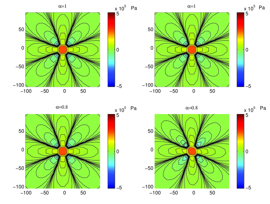
Figure 4: Map of the shear stress transfer $\sigma_{xy}$ for $\alpha=1$ and $\alpha=0.8$ in the pure shear stress load case (left panels) and in the pure shear strain loading case (right panels). The source is located at $(0,0)$ and all space units are kilometers.

Figures 4 to 6 show the variation of the shear stress component $\sigma_{xy}$ within the plate near the source cell. A positive variation signifies that this stress component increases. On each figure, the panels on the left represent patterns obtained with the pure shear stress load hypothesis, while the panels on the right represent patterns obtained with the pure shear strain load hypothesis. Each row corresponds to a different value of $\alpha$, i.e., to a different degree of elastic asymmetry between extensive and compressive deformation.

In the case $\alpha=1$, both boundary conditions yield exactly the same spatial pattern, as expected. This is in agreement with the fact that, in linear elasticity, both boundary conditions are equivalent. We obtain $8$ lobes of identical shapes within which stress amplitude alternates from positive to negative (red and blue lobes, repectively).

As $\alpha$ decreases, the symmetry of the patterns decreases: some lobes are rotating, some are widening while others are narrowing. We will study stress variation in those lobes in a subsequent section. The most striking observation is however that the spatial structure of the patterns is the same for both types of boundary conditions for a given value of $\alpha$, notwithstanding a significantly smaller stress amplitude in the pure shear strain load boundary condition.

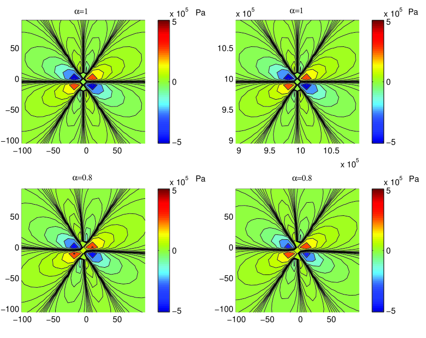
Figure 7: Map of the stress transfer $\sigma_{xx}$ for $\alpha=1$ and $\alpha=0.8$ in the pure shear stress load case (left panels) and in the pure shear strain loading case (right panels). The source is located in $(0,0)$ and all space units are kilometers.

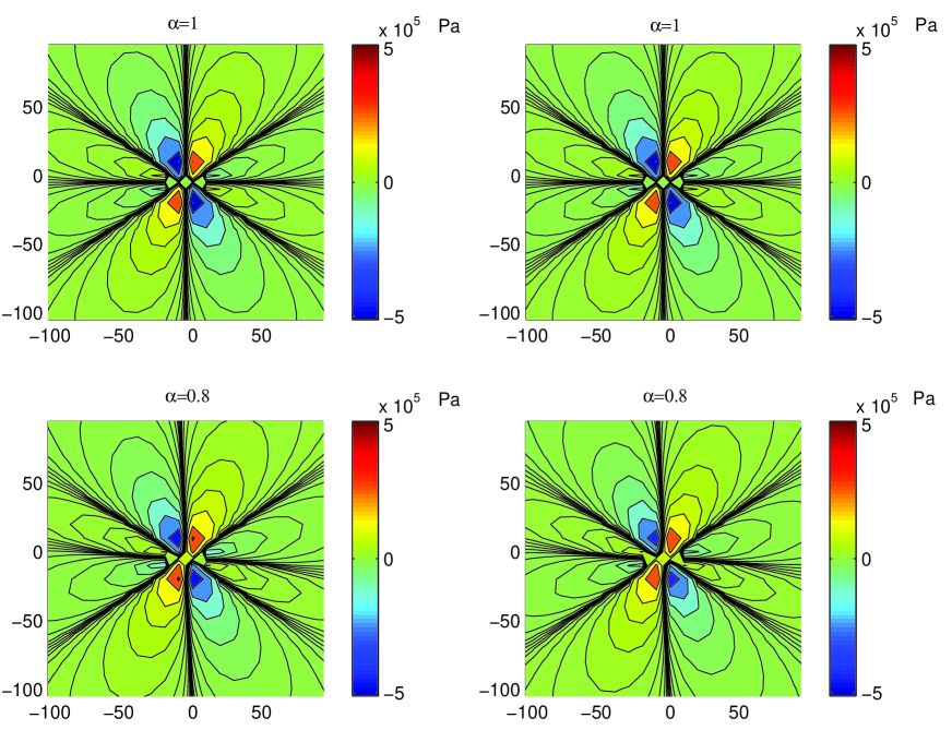
Figure 10: Map of the stress transfer $\sigma_{yy}$ for $\alpha=1$ and $\alpha=0.8$ in the pure shear stress load case (left panels) and in the pure shear strain loading case (right panels). The source is located in $(0,0)$ and all space units are kilometers.

Figures 7 to 9 show the variation of the stress component $\sigma_{xx}$ within the plate. The same kind of comments apply here as for $\sigma_{xy}$. This is also the case for component $\sigma_{yy}$ which is shown in Figures 10 to 12.

We have thus introduced a mechanical asymmetry at the microscopical level (i.e. at the spring scale), for all springs’orientations corresponding to an isotropic asymmetry, which translates into a loss of symmetry at the macroscopical scale. We shall quantify this loss of symmetry more precisely in the next section.

7.2 Decay of the stress amplitude away from the source

If we consider the center of the source cell as the origin of our frame, every point within the plate can be located using polar coordinates $(r,\theta)$, where $r$ is the distance to the origin (the source cell center), and $\theta$ is an azimuth measured clockwise from the $\vec{O}_{x}$ axis. We can then, for a fixed $\theta$, look at the decay rate with $r$ of the modulus of any of the stress tensor components. To avoid problems due to the finite size of the source and of the whole plate, we quantify the decay of the modulus of any stress component by a power-law of the type $r^{-\gamma}$, within a distance interval bracketed within a few cell to a few tens of cell sizes. We then repeat the same computation for different values of $\theta$. We then change the value of the asymmetry factor $\alpha$ and obtain the corresponding dependences $\gamma(\theta)$ for each value of $\alpha$.

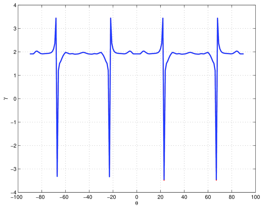
Figure 13: Variation of the decay exponent $\gamma$ with azimuth $\theta$ when $\alpha=1$ measured for the stress component $\sigma_{xy}$. The values of $\gamma$ obtained with pure shear stress loading and pure shear strain loading superimpose exactly. All values of $\gamma$ are close to the theoretical value $\gamma=2$ for symmetric elasticity, except at stress lobes borders where it is ill-defined numerically and exhibits spurious peak values.

Figures 13 to 15 show the variation of $\gamma$ with $\theta$, for different values of $\alpha$, quantifying the decay of the $\sigma_{xy}$ component. Each frame features two curves, one corresponding to the pure shear stress condition at the source (in red), the other one to the pure shear strain condition (in blue).

When $\alpha=1$, $\gamma$ is very close to $2$, which is the theoretical value predicted by planar elasticity. There are some small fluctuations around that value, the largest ones being obtained for values of the azimuth corresponding to a change of sign of the stress, i.e. where the stress itself almost vanishes. In those peculiar directions, the determination of the exponent is very unstable.

When $\alpha$ decreases, $\gamma$ values can reach values very different from $2$. Some of those values correspond to azimuths where stress vanishes (and are thus spurious), but others reflect genuine consequences of the nonlinearity of the medium. One can see that exponents can thus reach values larger than $2$ (reflecting a very rapid decay and thus short interaction range), but that they can also get down to values around or lower than $1$, leading to very large interaction ranges. When $\alpha=0.01$, one should not consider negative values of $\gamma$ too seriously as such negative values would imply that the stress increases with distance. The increase is occurring only over a finite distance range and gives way to a decrease at larger distance. The measured exponent is thus only valid at very short distances and is not an asymptotic value. We are unable for those cases to quantify accurately the value of the asymptotic $\gamma$ due to finite size effects. For that $\alpha$ values, one should thus consider that the asymptotic value of $\gamma$ varies en general between $0$ and $1$.

The found values of $\gamma$ as a function of $\theta$ also reveal that exponents do not vary significantly with the conditions imposed at the source, which constitutes another surprise. However, stresses obtained in the pure shear strain condition are lower than in the pure shear stress condition, as the prefactor of the power-law decay is found smaller than for the pure shear stress case.

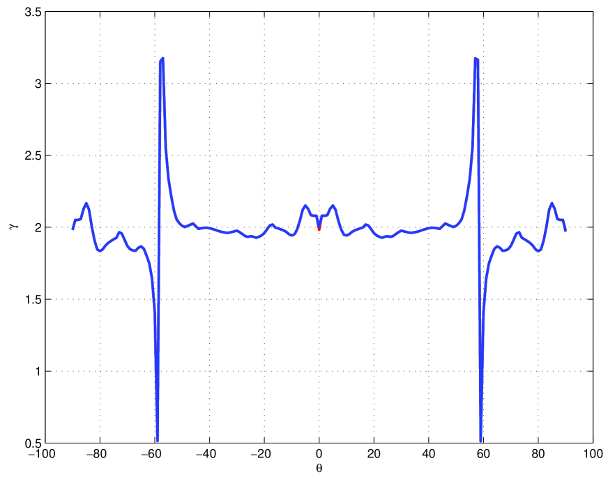
Figure 16: Variation of the decay exponent $\gamma$ with azimuth $\theta$ for $\alpha=1$ for the stress component $\sigma_{xx}$. The values of $\gamma$ obtained with pure shear stress and pure shear strain loading superimpose exactly. $\gamma$ is found close to the theoretical value $2$, except at stress lobe borders where it is ill-defined and exhibits spurious peak values.

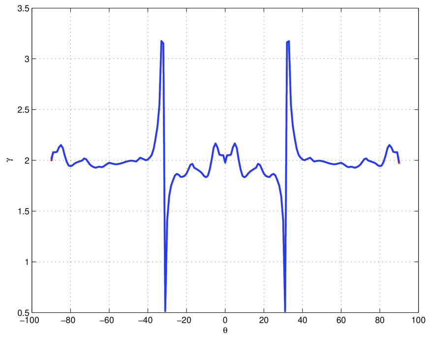
Figure 19: Variation of the decay exponent $\gamma$ with azimuth $\theta$ for $\alpha=1$ for the stress component $\sigma_{yy}$. The values of $\gamma$ obtained with pure shear stress and pure shear strain loading superimpose exactly. All values of $\gamma$ are close to the theoretical value $\gamma=2$, except at stress lobe borders where they are ill-defined and exhibit spurious peak values.

Figures 16 to 18, as well as Figures 19 to 21 show the same results for components $\sigma_{xx}$ and $\sigma_{yy}$. For both components, and for $\alpha=1$, we recover the theoretical value $\gamma=2$ for any $\theta$. As $\alpha$ decreases, the exponents can take very different values, including some which imply very long range decay. We observe again that the exponents do not vary with the type of loading at the source. We also checked that the explaination for negative values of exponents was the same as for $\sigma_{xy}$. Thus, for low $\alpha$ values, $\gamma$ decreases to values between $0$ and $1$.

8 Discussion

This idea of mechanical asymmetry, and/or of the feedback between local damage and stress decay from perturbative sources is not new but, to the best of our knowledge, it is the first time that it is implemented in a real $2D$ plane elastic problem applied to Earth mechanics and seismotectonics. For example, [51] gives the analytical solution for the stress field and for the dependence $\gamma(\alpha)$ in a nonlinear asymmetric elastic medium in the case of antiplane mode III loading, which is thus the scalar equivalent to the problem studied here. In the antiplane case, there is only one stress component and a single exponent $\gamma(\alpha)$. In this antiplane case, it can be shown analytically that the exponent $\gamma(\alpha)$ is indeed decreasing from the value $2$ for $\alpha=1$ to smaller values as $\alpha$ decreases. But there is not dependence on azimuth for this scalar case.

The existence of an asymmtry in the crust elasticity has been proposed on the basis of observations of the Manyi ($Mw=7.6$) earthquake [49]. Using SAR interferometry data, Peltzer et al. [49] interpreted the mismatch between the displacement across each side of the left-lateral strike-slip fault as due to a mechanical asymmetry between dilational and compressional quadrants. Using a first-order perturbative calculation, they estimated a coefficient $1/4\leq\alpha\leq 1/2$ to explain the observed displacement asymmetry. However, they did not consider the possibility the asymmetry could modify the long range decay rate of the stress field. This in turn can modify the future seismic history in the neighborhood of this event. Their computation showed that the asymmetric effect was probably confined in the very shallow part of the crust which, if true, implies that the stress transfer at seismogenic depths after this event obeys standard linear elastic solutions.

The fact that this model should be relevant for shallow crustal mechanics is rather obvious (as shown from the previous field example as well as from the short discussion at the beginning of this paper). The important question is to check if this model also holds (at least in limited spatial domains) at depth. In that case, stress transfer case-studies should take account of this asymmetry effect, which can greatly enhance the distance at which a given event can trigger another one. Testing this hypothesis is not simple, as the rheology we assumed is nonlinear, which means that the effect of successive events can not be simply added. Stress field evolutions with time may then have much sharper transitions in space and time than predicted by models involving linear elasticity, a behaviour reminiscent of the mechanics of granular media [50]. The consequence is that, to compare with the standard stress transfer mechanism [1], we need to know in details the state of stress within the crust prior to an event to map predicted stress transfer lobes onto aftershocks location catalogs.

Another possibility for testing our hypothesis would be to study the statistics of seismic moment tensors of events, as we saw that, if we assume that the source can be describe dynamically as a pure double couple of forces, this tensor should display a non-vanishing isotropic part. However, the seismic moment tensor is computed from seismic wave observations (i.e. of dynamical nature), and not from static displacements in situ at depth. Morover, the time at which the solutions we computed really hold depends on the diffusion properties of fluids in rock. This is why such a way of testing would indeed imply to compute the whole time-dependent dynamical asymmetric poro-elastic solution to really propose quantitative results allowing a reliable comparison.

Other data that could be used to test the model are the SAR data, in the spirit of the work of [49]. Interpretation of SAR data done after a large event could prove the pertinence of our model, provided that stress field evolution after the event is not modified by other events or by the far-field loading of the plate.

Proving or refuting this model is of prime importance for the understanding of the spatio-temporal patterns of earthquakes, including those preceeding a large and potentially destructive event. We already discussed the fact that it could improve the potential of prediction methods based on concepts such as stress transfer. But it has even deeper implications on the hope of predicting large events from the behavior of the statistics of populations of shocks preceeding that event. In another numerical work, Ref. [52] studied the progressive damage of a fault plane before its macroscopic rupture. Their model employs cellular automaton techniques to simulate tectonic loading, rupture events and strain redistribution. Note that in that case, strain is equivalent to stress. The elastodynamic Green function for stress/strain redistribution is taken to vary as $1/r^{p}$, where $p$ is a parameter which is varied. The systems displays two different regimes depending on the $p$ value. For $p\leq 2$, large events are preceeded by a clear power-law acceleration of energy release of the system, together with the growth of strain energy correlations. This is of course reminiscent of the critical earthquake hypothesis [13, 16, 17]. For $p$ larger than $2$, the trend of energy release before a large event is linear. This means that the lower $p$ is, the more predictable is the large event, using time series of precursory energy release. Their model does not map exactly to ours,, but we could expect that if $\alpha$ is under a certain threshold (still to be determined), then $\gamma$ would be low enough for the critical earthquake scenario to apply, making large events predictable from time series. In the other hand, if in some areas $\alpha$ is above that threshold, then the local tectonic domain would belong to the other regime, and large events would be unpredictable. If the predictability of large events relies, as suggested by [52], on the exponent of the Green function of stress transfer, then we have pointed out a very simple physical mechanism allowing to tune that exponent. Large scale fluctuations of fluid pressure from lithostatic to infra-lithostatic could then explain why in some cases large events are preceeded by strain energy release acceleration, while the opposite holds in other cases.

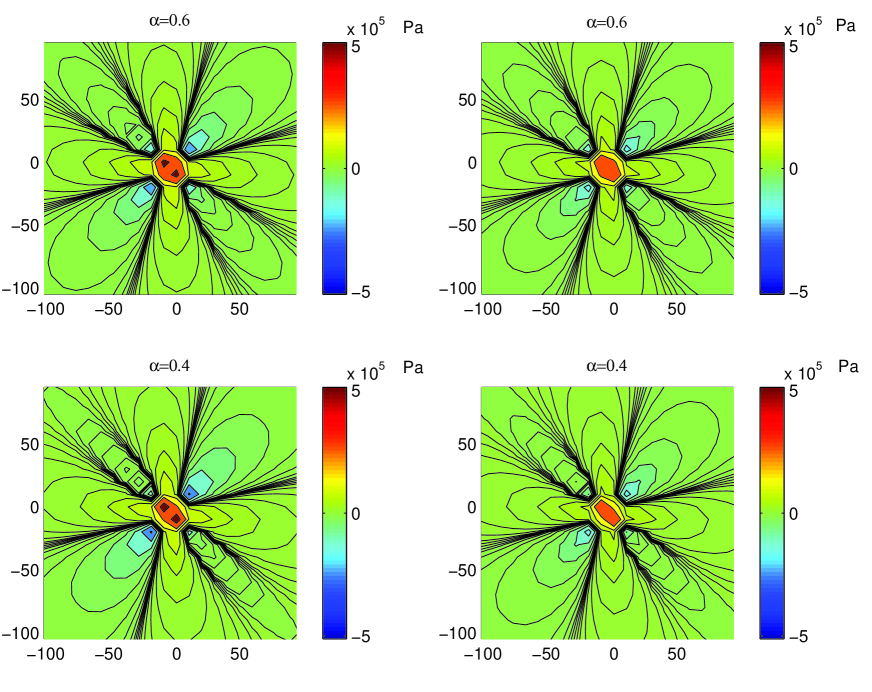
Figure 5: Same as Fig. 4 for $\alpha=0.6$ and $\alpha=0.4$.

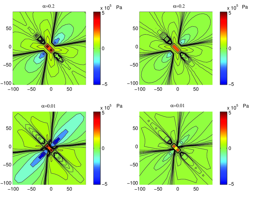
Figure 6: Same as Fig. 4 for $\alpha=0.2$ and $\alpha=0.01$.

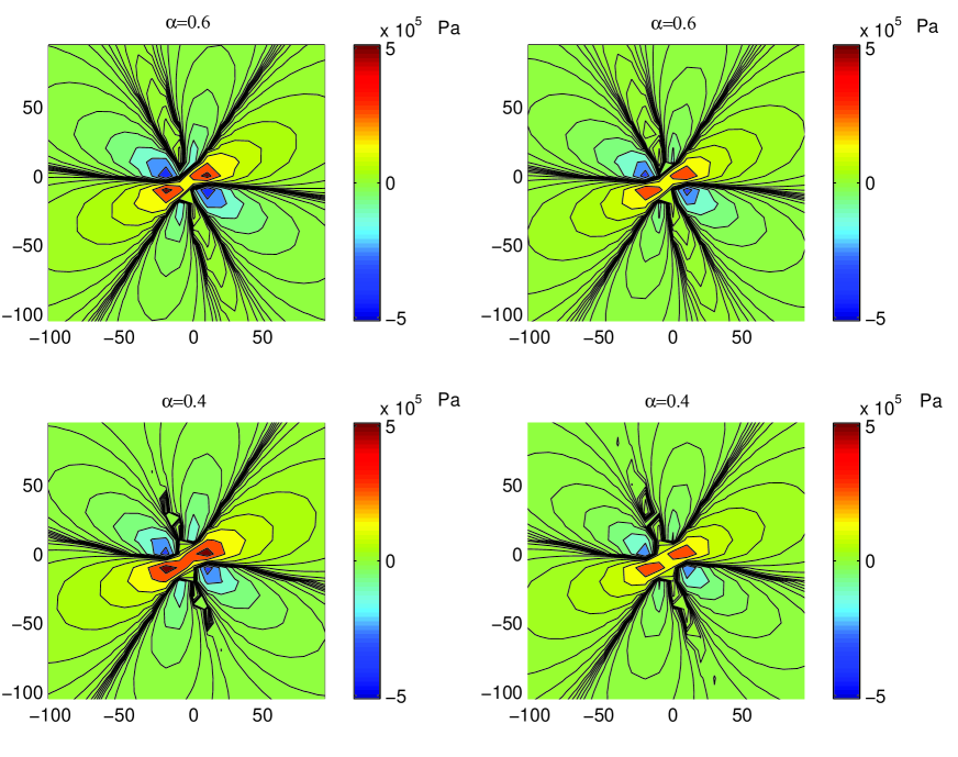
Figure 8: Same as Fig. 7 for $\alpha=0.6$ and $\alpha=0.4$.

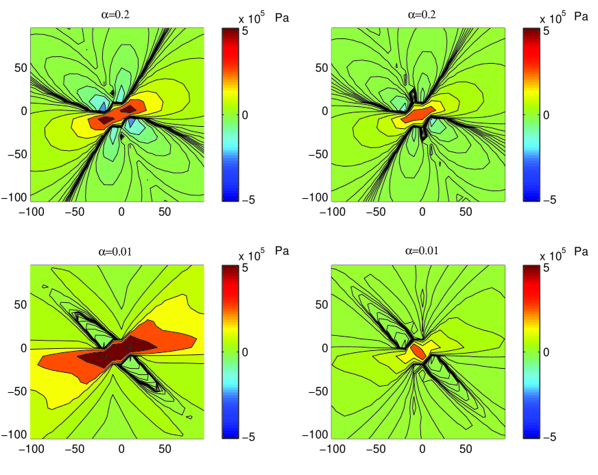
Figure 9: Same as Fig. 7 for $\alpha=0.2$ and $\alpha=0.01$.

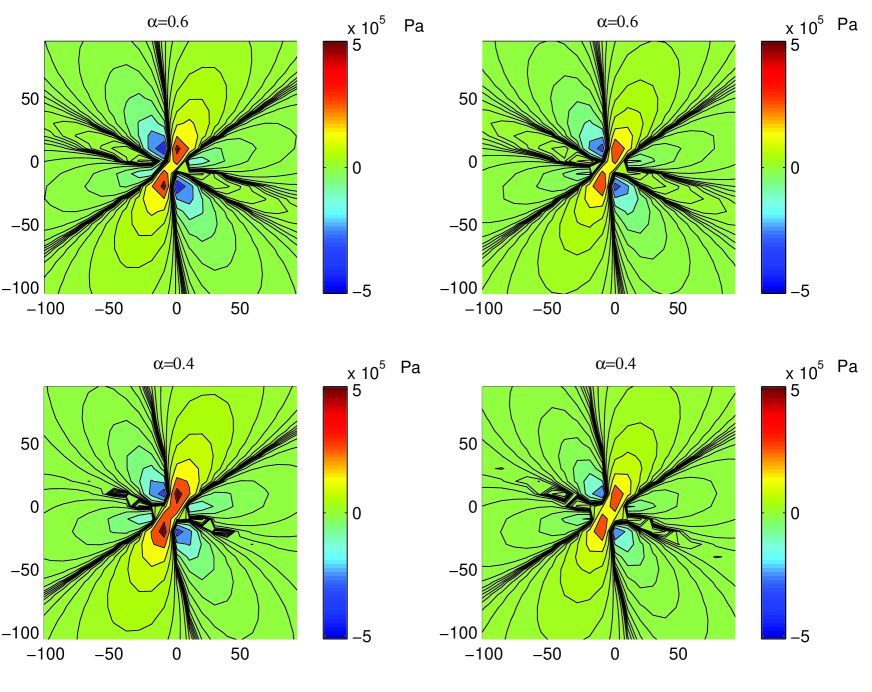
Figure 11: Same as Fig. 10 for $\alpha=0.6$ and $\alpha=0.4$.

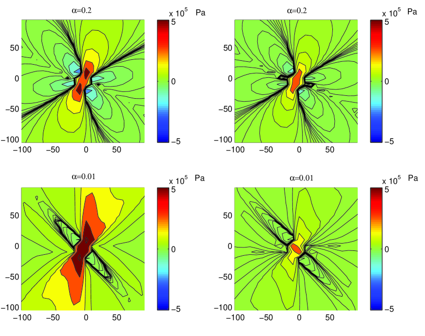
Figure 12: Same as Fig. 10 for $\alpha=0.2$ and $\alpha=0.01$.

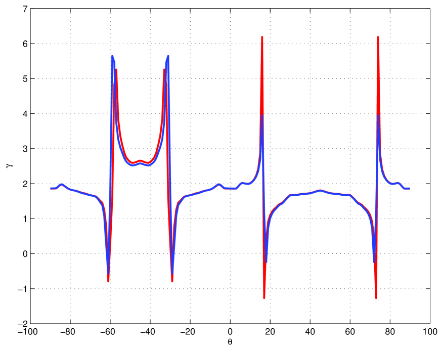
Figure 14: Variation of the decay exponent $\gamma$ with azimuth $\theta$ for $\alpha=0.5$ for the stress component $\sigma_{xy}$. The red (respectively blue) curve is for pure shear stress (respectively pure shear strain) loading. Peak values are spurious and correspond to lobes boundaries. The exponents are essentially identical for both types of loading conditions.

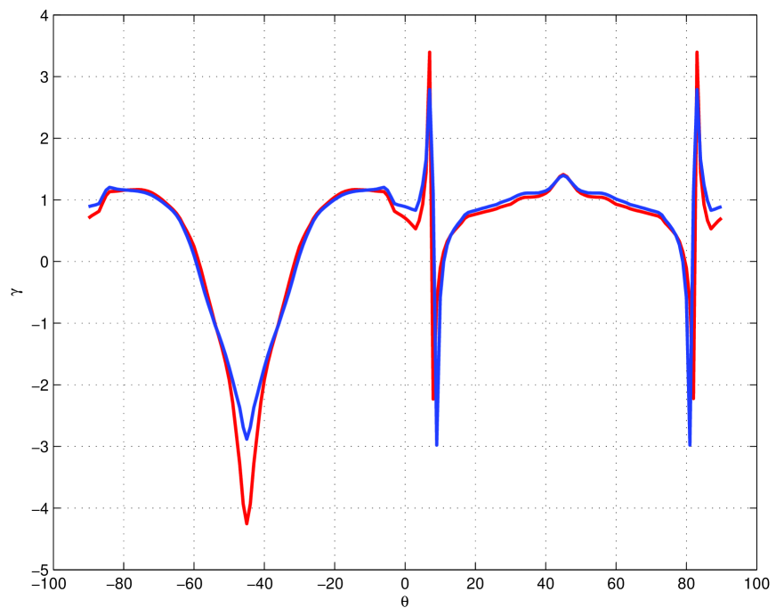
Figure 15: Same as Fig. 14 for $\alpha=0.01$.

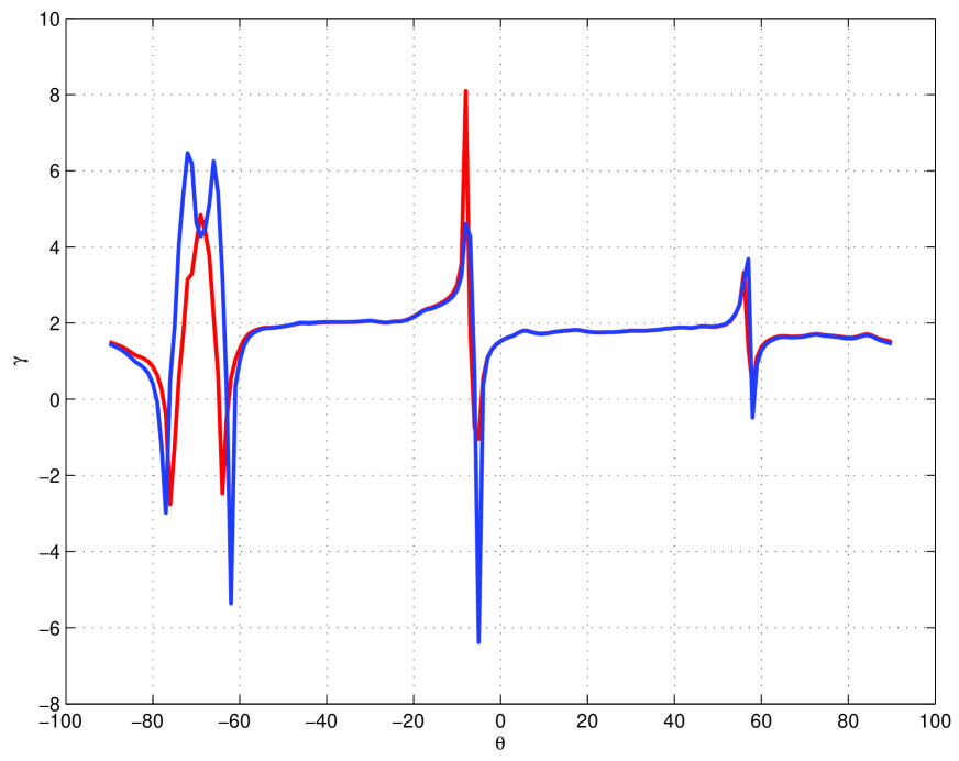
Figure 17: Same as Fig. 16 for $\alpha=0.5$. The red (respectively blue) curve is for pure shear stress (respectively strain) loading. Peak values are spurious and correspond to lobe boundaries. The exponents are very similar for both types of loading conditions.

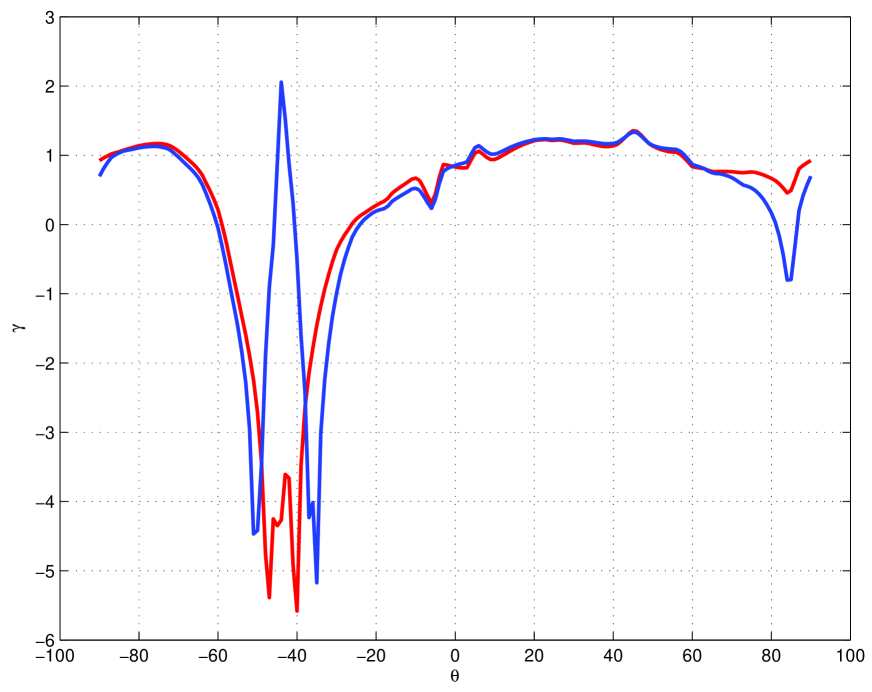
Figure 18: Same as Fig. 16 for $\alpha=0.01$.

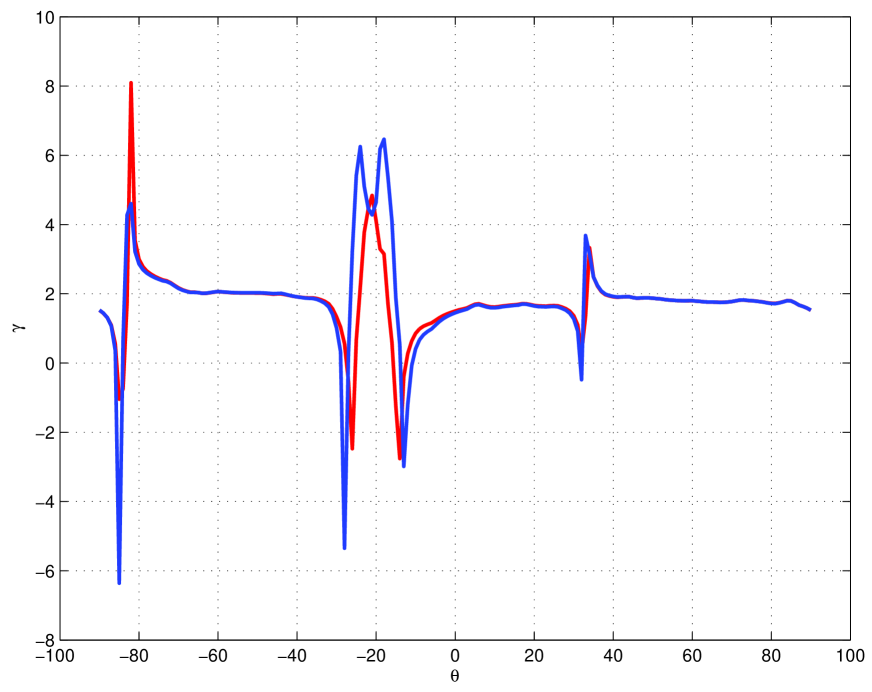
Figure 20: Same as Fig. 19 for $\alpha=0.5$. The red (respectively blue) curve is for pure shear stress (respectively strain) loading. Peak values are again spurious and correspond to lobe boundaries. The exponents are very similar for both types of loading conditions.

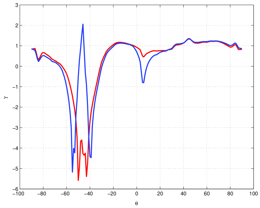
Figure 21: Same as Fig. 20 for $\alpha=0.01$.

References

- [1] R.S. Stein, Nature 402, 605 (1999).
- [2] A. Cochard and Madariaga R., Dynamic faulting Pure and Appl. Geophys 142, 419 (1994).
- [3] K. Aki and Richards P.G., Quantitative Seismology, University Science Books (2002)
- [4] N. Lapusta, Rice, J.R., Ben-Zion, Y. and Zheng, G.T., J. Geophys. Res. 105, 23765 (2000).
- [5] D. Sornette D., P. Miltenberger and C. Vanneste, Pure and Appl. Geophys., 142, 491 (1994).
- [6] Y. Ben-Zion,Dahmen, K., Lyakhovsky, V., Ertas, D. and D. Fisher, Earth and Planet. Sci. Lett. 172, 11 (1999).
- [7] A. Gabrielov, Keilis-Borok,V. and Jackson, D.D., Proc. Natl. Acad. Sci. USA 93, 3838 (1996).
- [8] R.A. Harris, Current Science 79, 1215 (2000).
- [9] Harris, R.A., Dolan, J.F., Hartleb, R. and Day, S.M., Bull. Seism. Soc. Am. 92, 245 (2002).
- [10] R.A. Harris and Simpson, R.W., J. Geophys. Res. 103, 24439 (1998).
- [11] R.A. Harris, Simpson, R.W. and Reasenberg, P.A., Nature 375, 221 (1995).
- [12] V.I. Keilis-Borok and L. N. Malinovskaya, J. Geophys. Res., 69, 3019 (1964).
- [13] D.D. Bowman, G. Ouillon, C.G. Sammis, A. Sornette and D. Sornette, J. Geophys. Res. 103 (NB10), 24359-24372 (1998).
- [14] L.M. Jones and P. Molnar, J. Geophys. Res., 84, 3596 (1979).
- [15] L. Knopoff, T. Levshina, V.I. Keilis-Borok and C. Mattoni, J. Geophys. Res., 101, 5779 (1996).
- [16] S.C. Jaumé and Sykes, L.R., Pure Appl. Geophys., 155, 279 (1999).
- [17] S.G. Sammis and D. Sornette, Proc. Nat. Acad. Sci. USA, 99, 2501 (2002).
- [18] D. Kilb, J. Gomberg, P. Bodin, J. Geophys. Research 107, doi10.1029/2001JB000202 (2002).
- [19] J. Gomberg, J. Geophys. Res. 106, 16253 (2001)
- [20] E. Roeloffs and E. Quilty, Pure Appl. Geophys. 149, 21 (1997).
- [21] National Research Council, The role of fluids in crustal processes, Studies in geophysics, Geophysics study committed, Commission on Geosciences, Environment and Ressources, National Academic Press, Washington D.C. (1990).
- [22] D. Sornette, Phys. Rep. 313, 238 (1999).
- [23] Walther, J.V., Fluid Dynamics During Progressive Regional Metamorphism, in [21], 64.
- [24] Nur, A., and J. Walder, Time-Dependent Hydraulics of the Earth’s Crust, in [21], 113.
- [25] Lachenbruch, A.H., J. Geophys. Res., 85, 6097 (1980).
- [26] Byerlee, J., Geophys. Res. Lett., 17, 2109 (1990).
- [27] Rice, J.R., in Fault mechanics and transport properties in rocks (the Brace volume), ed. Evans, B., and T.-F. Wong, Academic, London, 475 (1992).
- [28] M.L. Blanpied, D.A. Lockner and J.D. Byerlee, J. Geophys. Res., 100, 13045 (1995).
- [29] Sleep, N.H., and M.L. Blanpied, Nature, 359, 687 (1992).
- [30] Moore, D.E., et al., Geology, 24, 1041 (1996).
- [31] Hickman, S., R. Sibson and R. Bruhn, J. Geophys. Res., 100, 1283 (1995).
- [32] Wintsch, R.P., R. Christoffersen and A.K. Kronenberg, J. Geophys. Res., 100, 13021 (1995).
- [33] Robert, F., A.-M. Boullier and K. Firdaous, J. Geophys. Res., 100, 12861 (1995).
- [34] Burst, J.P., American Association of Petroleum Geologists Bulletin, 53, 73 (1969).
- [35] R.H. Sibson, in Earthquake prediction, an international review, Amer. Geophys. Union, D.W. Simpson and P.G. Richards, eds., Maurice Ewing Ser., 4, 593 (1982).
- [36] A. Nur and J.R. Booker, Science, 175, 885 (1972).
- [37] C.H. Scholz, The mechanics of earthquakes and faulting (Cambridge [England]; New York: Cambridge University Press, 1990).
- [38] J.C. Jaeger and N.G. Cook, Fundamentals of rocks Mechanics (Chapman & Hall, London, ed. 3, 1979).
- [39] R.A. Guyer and P.A. Johnson, Phys. Today, 52, 30 (1999) and other results at http://www.ees4.lanl.gov/nonlinear/
- [40] P. Wannamkaer, Resistivity images imply a zone of active fluid production from prograde metamorphism in the lower crust, and transport of fluids to shallower levels along major fore- and backthrusts, Collaborative Research: Magnetotelluric Transect of a Modern Continent-Continent Collisional Orogen: Southern Alps, New Zealand.
- [41] S. Kirby, A possible deep, long-term source of pressurized water for the San Andreas Fault system: A ghost of Cascadia subduction past? USGS, Menlo Park (2003).
- [42] A. Attila, Lattice dynamical foundations of continuum theories: elasticity, piezoelectricity, viscoelasticity, plasticity (Singapore: World Scientific and Taylor & Francis, 1986).
- [43] H.D. Garbin and L. Knopoff, Q. appl. Math. 33, 301 (1975).
- [44] L. Monette and M. P. Anderson, Modelling Simul. Mater. Sci. Eng. 2, 53 (1994).
- [45] R. Burridge and L. Knopoff, Bull. Seism. Soc. Am. 54 (1), 1875 (1964).
- [46] J. Pujol. Seismological Research Letters 74 (2), 163 (2003).
- [47] Kuge, K., and T. Lay, J. Geophys. Res. 99, 15457 (1994).
- [48] Frohlich, C., Science 264, 804 (1994).
- [49] G. Peltzer, F. Crampé and G. King, Science 286, 272 (1999).
- [50] M.E. Cates, Wittmer J.P., Bouchaud J.-P., Claudin P., Phys. Rev. Lett. 81, 1841 (1998).
- [51] S. Roux and F. Hild, Int. J. Fract. 116, 219 (2002).
- [52] D. Weatherley, Mora P. and Xia M. (2003).