[

Universal behavior of localization of residue fluctuations in globular proteins

Abstract

Localization properties of residue fluctuations in globular proteins are studied theoretically by using the Gaussian network model. Participation ratio for each residue fluctuation mode is calculated. It is found that the relationship between participation ratio and frequency is similar for all globular proteins, indicating a universal behavior in spite of their different size, shape, and architecture.

]

Proteins are important biological macromolecules that control almost all functions of living organisms. It was once believed that proteins are rather amorphous and without well-defined structures. After more and more structures have been determined by crystallographic and NMR methods, it has revealed that protein structures are far from random. They have well-defined secondary and tertiary structures which comprise essential information relating to their functions and mechanisms.

Proteins in the folded states are not static. Instead, the constituent residues fluctuate near their native positions owing to the finite temperature effects[2]. It has been now well accepted that the fluctuations are crucial for enzyme catalysis and for biological activity[3, 4]. Recently, there has been considerable interest in the correlations between protein functions and fluctuations[3]. Intensive theoretical studies on fluctuations of protein have been carried out based on either molecular dynamics simulations or normal mode analyses (NMA) by using all-atom empirical potentials[5]. It has been shown that the NMA is a very useful method to study protein fluctuations[6, 7]. The use of atomic approaches becomes computational demanding when dealing with large proteins. For proteins composed of more than thousand residues, it is difficult to investigate by using the conventional atomic models and potentials. On the other hand, coarse-grained protein models and simplified force fields have revealed a great success in description of the residue fluctuations of proteins[8, 9, 10, 11]. Although there have been intensive studies on residue fluctuations, to our knowledge, there is few study on localization properties of residue fluctuations.

In this paper, based on a coarse-grained protein model, we show theoretically that there is a similar behavior in the localization of residue fluctuations for globular proteins, even though their architectures and sizes are rather different. In our study of residue fluctuations, proteins are modeled as elastic networks. The nodes are residues linked by inter-residue potentials that stabilizes the folded conformation. This model has been usually referred as the Gaussian network model (GNM), which can give a satisfactory description of the fluctuation of folded proteins[9, 10, 12, 13, 14, 15, 16]. In this model, residues are assumed to undergo Gaussian-distributed fluctuations about their native positions. No distinction is made between different types of residues. A single generic harmonic force constant is used for the inter-residue interaction potential within a cutoff range. We consider residues as the minimal representative units and the $\alpha$-carbons are used as corresponding sites for residues. Considering all contacting residues, the internal Hamiltonian within the GNM is given by[9, 10]

$$H=\frac{1}{2}\gamma\left[\Delta{\bf R}^{\text{T}}\left({\bf\Gamma}\otimes{\bf E}\right)\Delta{\bf R}\right],$$ (1)

where $\gamma$ is the harmonic force constant; $\left\{\Delta{\bf R}\right\}$ represents the $3N$-dimensional column vectors of fluctuations $\Delta{\bf R}_{1},\ldots,\Delta{\bf R}_{N}$ of the $C^{\alpha}$ atoms, where $N$ is the number of residues; ${\bf E}$ is the third order identity matrix; the superscript T denotes the transpose; $\otimes$ stands for the direct product, and ${\bf\Gamma}$ is the $N\times N$ Kirchhoff matrix[17] with the elements given by

$$\Gamma_{ij}=\left\{\begin{array}[]{ll}-H\left(r_{\text{c}}-r_{ij}\right),&i\neq j,\\ -\sum\limits_{i(\neq j)}^{N}\Gamma_{ij},&i=j.\end{array}\right.$$ (2)

Here, $r_{ij}$ is the separation between the $i$-th and $j$-th $C^{\alpha}$ atoms; $H(x)$ is the Heaviside step function, and $r_{\text{c}}$ is the cutoff distance outside of which there is no inter-residue interaction. The $i$-th diagonal element of $\Gamma$ characterizes the local packing density or the coordination number of residue $i$. The inverse of the Kirchhoff matrix can be decomposed as

$$\Gamma^{-1}={\bf U}\Lambda^{-1}{\bf U}^{\text{T}},$$ (3)

where ${\bf U}$ is an orthogonal matrix whose columns ${\bf u}_{i}\left(1\leq i\leq N\right)$ are the eigenvectors of $\Gamma$, and $\Lambda$ is diagonal matrix of eigenvalue $\lambda_{i}$ of $\Gamma$. Cross-correlations of residue fluctuations between the $i$-th and $j$-th residues are found from

$$\left[\Delta{\bf R}_{i}\cdot\Delta{\bf R}_{j}\right]=\frac{3k_{B}T}{\gamma}\left[\Gamma^{-1}\right]_{ij}.$$ (4)

From Eqs. (3) and (4), the mean-square (ms) fluctuations (also called Debye-Waller or B-factors) of the $i$-th residue associated with the $\alpha$-th mode are given by

$$\left[\Delta{\bf R}_{i}\cdot\Delta{\bf R}_{i}\right]_{\alpha}=\frac{3k_{B}T}{\gamma}\lambda_{\alpha}^{-1}\left[u_{\alpha}\right]_{i}\left[u_{\alpha}\right]_{i}.$$ (5)

In our calculation, the cutoff distance $r_{\text{c}}=7$ Å is used, as adopted in previous studies[9, 10]. The harmonic force constant $\gamma$ is determined by fitting to the experimental ms fluctuations. From this model, one can obtain the fluctuation mode frequencies and eigenvectors for a given protein. The GNM can in general give results in good agreement with the observed B-factors [9, 10].

The spatial distribution of a given mode is characterized by its eigenvectors. To study the localization properties of protein fluctuations, we have to compute participation ratio (PR) for each mode, defined by[18]

$$P_{\alpha}=\frac{1}{N}\left(\sum\limits_{i}\left[u_{\alpha}\right]_{i}^{4}\right)^{-1}.$$ (6)

Values of PR range from $1/N$ to unity. PR takes the value of unity if all residues have equal fluctuation. If only one residue fluctuates PR is equal to $1/N$. From its definition, it is obvious that PR is a measure of the degree of localization. If the PR is small for a given mode, only a few residues have considerable fluctuations and the mode is a localized one. On the other hand, if the PR is large for a given mode, the mode is delocalized.

It is known that at the physiological temperatures, protein fluctuates among different conformations around its native one. Therefore, in principle, all contributions from these conformations should be considered in the calculation of PR. Unfortunately, only one conformation could be obtained from experiments. However, these conformations could be obtained approximately by the following way. For each residue, it is assumed that it can stay at any position inside the sphere with a radius of half the magnitude of fluctuation centered on the position obtained from experiments. A conformation can be derived by a random choice of the position for each residue while the inter-distance between two adjacent residues is kept unchanged within the framework of the SHAKE algorithm [19].

The calculated PR for several proteins is shown in Fig. 1. The Brookhaven Protein Databank (PDB) codes and references of the proteins studied are listed in Table I. The modes are numbered starting from the lowest frequency. In the calculations about 100 conformations are adopted. It is found that if more conformations are used, the curves will become smoother eventually.

Based on the Anderson localization theory[24, 25], Bahar et al. [10] suggested that modes with larger fluctuation frequencies would be more localized, indicating a monotonous decrease in PR with frequency. As suggested by Onuchic et al. [26] proteins are neither ordered nor random systems, the localization properties of protein fluctuations should show some intrinsic features from those in ordered or random systems.

It can be seen from Fig. 1 that starting from lowest frequency, PR first decreases with frequency, then increase, and finally decreases with frequency. A large number of globular proteins which have diversified topology, secondary structure arrangement and size are calculated. This behavior of PR seems to be universal, holding for all globular proteins. Other molecular systems such as tRNA are also calculated. But the behavior of PR is qualitatively different from proteins (data not shown). So it is reasonable to conjecture that the different behavior of PR in globular proteins from other systems reflects the intrinsic difference of certain properties. Recently, Micheletti et al. [28] studied the localization properties of HIV-1 protease. A similar behavior of PR in HIV-1 protease was found.

To study the origin of the behavior of PR in globular proteins, the fluctuation patterns of the protein myoglobin at different frequency regions are given in Fig. 2. The different frequency regions in the figure are labeled by different letters (see Fig. 1). In the low frequency region A, the fluctuations represent a collective motion, characterized by large values of PR. In the region B, the PR is small, implying localized fluctuations. It is interesting to note that in this region the fluctuations occur dominantly at the loops. In the highest frequency region D, the fluctuations are found to be confined to the secondary structures, resulting small PR. In the region C, one can find that motions of both loops and secondary structures are involved. The degree of localization is, however, smaller than that in regions B and D, but it is larger than that in region A. Therefore, it can be concluded from the fluctuation patterns that the dip of PR occurred at lower frequency side (region B) originates from the localized fluctuations at loops that connect the secondary structures. For conventional disordered solids or random coils, there are nearly no well-defined secondary structures and consequently no loops. The resulting PR will show a different behavior. It is obvious that the different behavior of PR in globular proteins from that of conventional random solids or coils originates from the different nature of structures.

To get a deeper insight into how the localization properties are affected by the topology, a lattice model[27] with different length of the loop is adopted. In this model, a protein is represented by a self-avoiding chain of beads placed on a two-dimensional discrete lattice. In construction of this model protein, one must consider the fact that the secondary structure has higher packing density while the loop has lower packing density. A core region is introduced by making two helices contacted each other since cores, with higher packing density, are important to stabilize the whole structure. Our model protein shown in Fig. 3(a) consists of two helices, a connective loop, and a core. All residues (beads) are treated identically. In our calculations only the nearest neighbor interaction is considered.

Advantages of the lattice model are that we can change the structure as desired to get insight into how the residue fluctuations are affected by the changes in structures, which is difficult to do in real proteins. In Fig. 3(b) the calculated PR by the GNM for the model protein with different loop length is shown. The loop length is changed by moving the loop horizontally to the left or right. The curves are smoothed simply by adjacent averaging using 10 points. It is obvious that the PR of fluctuations in the simple model protein shows a similar behavior to that of real globular proteins. With increase in the loop length, the PR values of both the dip (region B in Fig. 1) and the peak (region C in Fig. 1) decrease. It can be seen from Fig. 3(c) that at the dip the fluctuations are dominant in the loop region. Again, the origin of the dip is the cause of the loop. For the highest frequency mode, the fluctuations dominantly occur at the helices, especially at the core region. The broad peak comprises modes which are more delocalized and worse defined. These peaks are relevant to the coupling motions among secondary structures.

In summary, localization properties of fluctuations in globular proteins were studied by using the Gaussian network model. It was found that the participation ratio of fluctuations in globular proteins shows a universal behavior, confirmed by theoretical calculations in both real globular and model proteins. The loops connecting the secondary structures are responsible for this feature.

This work was supported by the NSFC. Partial support from Shanghai Science and Technology Commission, China is acknowledged. Interesting discussions with Dr. Y. Q. Zhou, Dr. C. Tang, and Dr. J. Z. Y. Chen are acknowledged.

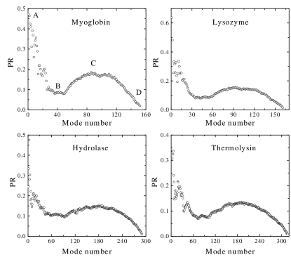
FIG. 1.: Calculated participation ratio of residue fluctuations for proteins listed in Table I.

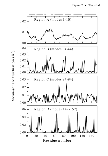
FIG. 2.: Calculated projected residue ms fluctuations in different frequency regions for myoglobin. The secondary structures of myoglobin are represented by the horizontal segment heavy lines at the top of the figure. The remaining are loops.

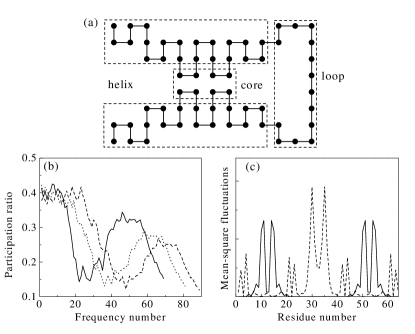
FIG. 3.: (a) Lattice model protein consists of two helices, a loop and a core region. The loop length can be changed by moving the loop horizontally to the right. (b) Participation ratio for model proteins with different loop length. Solid line is for the model protein shown in (a) with loop length of 13$a$, where $a$ is the lattice constant. Dotted and dashed lines are for model proteins with loop length of 23$a$ and 33$a$, respectively. (c) Projected residue ms fluctuations in arb. units for the modes with smallest PR in the dip region (dashed line) and with largest frequency (solid line).

TABLE I.: The PDB code and reference of proteins studied in the present work.

Protein	PDB code	Reference
Myoglobin Lysozyme Hydrolase Thermolysin	1bvc 166l 1amp 5tln	[20] [21] [22] [23]

REFERENCES

- [1] To whom all correspondence should be addressed. Electronic address: jzi@fudan.edu.cn
- [2] H. Frauenfelder, S. G. Sligar, and P. G. Wolynes, Science 254, 1598 (1991).
- [3] A. Stock, Nature 400, 221 (1999).
- [4] G. Zaccai, Science 288, 1604 (2000).
- [5] A. Kitao and N. Go, Curr. Opin. Struct. Biol. 9, 164 (1999) and references therein.
- [6] M. Levitt, C. Sander, and P. S. Stern, J. Mol. Biol. 181, 423 (1985).
- [7] S. Hayward, A. Kitao, and H. J. C. Berendsen, Proteins 27, 425 (1997).
- [8] M. M. Tirion, Phys. Rev. Lett. 77, 1905 (1996).
- [9] T. Haliloglu, I. Bahar, and B. Erman, Phys. Rev. Lett. 79, 3090 (1997).
- [10] I. Bahar et al., Phys. Rev. Lett. 80, 2733 (1998).
- [11] K. Hinsen and G. R. Kneller, J. Chem. Phys. 111, 10766 (1999).
- [12] I. Bahar and R. L. Jernigan, J. Mol. Biol. 266, 195 (1997); I. Bahar, A. R. Atilgan, and B. Erman, Fold. Des. 2, 173 (1997); I. Bahar and R. L. Jernigan, J. Mol. Biol. 281, 871 (1998); I. Bahar et al., Biochem. 37, 1067 (1998); I. Bahar et al., J. Mol. Biol. 285, 1023 (1999); I. Bahar and R. L. Jernigan, Biochem. 38, 3478 (1999).
- [13] M. C. Demirel et al., Protein Sci. 7, 2522 (1998).
- [14] R. L. Jernigan, M. C. Demirel, and I. Bahar, Int. J. Quant. Chem. 75, 301 (1999).
- [15] O. Keskin, I. Bahar, and R. L. Jernigan, Biophys. J. 78, 2093 (2000).
- [16] A. R. Atilgan et al., Biophys. J. 80, 505 (2001).
- [17] F. Harry, Graph Theory (Addison-Wesley, Reading, MA, 1971).
- [18] R. J. Bell, Rep. Prog. Phys. 35, 1315 (1972).
- [19] J. P. Ryckaert, G. Ciccotti G, H. J. C. Berendsen, J. Comput. Phys. 23, 327 (1977).
- [20] U. G. Wagner et al., J. Mol. Biol. 247, 326 (1995).
- [21] L. H. Weaver and B. W. Matthews, J. Mol. Biol. 193, 189 (1987).
- [22] C. Schalk et al., Arch. Biochem. Biophys. 294, 91 (1992).
- [23] M. A. Holmes and B. W. Matthews, Biochem. 20, 6912 (1981).
- [24] P. W. Anderson, Phys. Rev. 109, 1492 (1958).
- [25] P. W. Anderson, Rev. Mod. Phys. 50, 191 (1978).
- [26] J. N. Onuchic et al., Adv. Protein Chem. 53, 87 (2000).
- [27] K. A. Dill et al., Protein Sci. 4, 561 (1995).
- [28] C. Micheletti, G. Lattanzi, and A. Maritan, J. Mol. Biol. 321, 909 (2002).