Random walk with shrinking steps

Abstract

We outline the properties of a symmetric random walk in one dimension in which the length of the $n$th step equals $\lambda^{n}$, with $\lambda<1$. As the number of steps $N\to\infty$, the probability that the endpoint is at $x$ approaches a limiting distribution $P_{\lambda}(x)$ with many beautiful features. For $\lambda<1/2$, the support of $P_{\lambda}(x)$ is a Cantor set. For $1/2\leq\lambda<1$, there is a countably infinite set of $\lambda$ values for which $P_{\lambda}(x)$ is singular, while $P_{\lambda}(x)$ is smooth for almost all other $\lambda$ values. In the most interesting case of $\lambda=g\equiv(\sqrt{5}-1)/2$, $P_{g}(x)$ is riddled with singularities and is strikingly self-similar. The self-similarity is exploited to derive a simple form for the probability measure $M(a,b)\equiv\!\int_{a}^{b}P_{g}(x)\,dx$.

I INTRODUCTION

This article discusses the properties of random walks in one dimension in which the length of the $n$ step changes systematically with $n$. That is, at the $n$th step, a particle hops either to the right or to the left with equal probability by a distance $f(n)$, where $f(n)$ is a monotonic but otherwise arbitrary function. The usual nearest-neighbor random walk is recovered when $f(n)=1$ for all $n$.

Why should we care about random walks with variable step lengths? There are several reasons. First, for the geometric random walk, where $f(n)=\lambda^{n}$ with $\lambda<1$, a variety of beautiful and unanticipated features arise,W ; E ; G ; Kac as illustrated in Fig. 1. A very surprising feature is that the character of the probability distribution of the walk changes dramatically as $\lambda$ is changed by a small amount. Most of our discussion will focus on this intriguing aspect. We will emphasize the case $\lambda=g\equiv(\sqrt{5}-1)/2$, the inverse of the golden ratio, where the probability distribution has a beautiful self-similar appearance. We will show how many important features of this distribution can be obtained by exploiting the self-similarity, as well as the unique numerical properties of $g$.

There also are a variety of unexpected applications of random walks with variable step lengths. One example is spectral line broadening in single-molecule spectroscopy.BS Here the energy of a chromophore in a disordered solid reflects the interactions between the chromophore and the molecules of the host solid. For a dipolar interaction potential and for two-state host molecules with intrinsic energies $\pm\epsilon$, the energy of the chromophore is proportional to $\sum_{j}\pm\epsilon r_{j}^{-3}$, where $r_{j}$ is the separation between the chromophore and the $j$th molecule. This energy is equivalent to the displacement of a geometric random walk with $f(n)=n^{-3}$.

Another example is the motion of a Brownian particle in a fluid with a linear shear flow, that is, the velocity field is $v_{x}(y)=Ay$. As a Brownian particle makes progressively longer excursions in the $\pm y$ directions (proportional to $t^{1/2}$), the particle experiences correspondingly larger velocities in the $x$-direction (also proportional to $t^{1/2}$). This gives rise to an effective random walk process in the longitudinal direction in which the mean length of the $n$th step grows linearly with $n$, that is, $f(n)=n$.BRA

Historically, the geometric random walk has been discussed, mostly in the mathematics literature, starting in the 1930’s.W ; E Interest in such random walks has recently revived because of connections with dynamical systems.A ; L Recent reviews of the geometric random walk can be found in Ref. PSS, ; see also Ref. DF, for a review of more general iterated random maps. In contrast, there appears to be no mention of the geometric random walk in the physics literature, aside from Ref. junk .

Finally, the geometric random walk provides an instructive set of examples that can be analyzed by classical probability theory and statistical physics tools.reif ; weiss These examples can serve as a useful pedagogical supplement to a student’s introduction to the theory of random walks. As we shall discuss, there are specific values of $\lambda$ for which the probability distribution can be calculated by elementary methods, while for other $\lambda$ values, there is meager progress toward an exact solution, even though many tantalizing clues exist.

II Picture Gallery

The displacement of a one-dimensional random walk after $N+1$ steps has the form $x_{N}=\sum_{n=0}^{N}\epsilon_{n}f(n)$, where each $\epsilon_{n}$ takes on the values $\pm 1$ with equal probability. Consequently, the mean-square displacement $\langle x_{N}^{2}\rangle$ can be expressed as $\sum_{n}f(n)^{2}$. If this sum is finite, then there is a finite mean-square displacement as $N\to\infty$. In such a case, the endpoint probability distribution therefore approaches a fixed limit.bazant Henceforth, we will focus on the case of geometrically shrinking step lengths, that is, $f(n)=\lambda^{n}$ with $\lambda<1$. We denote the endpoint probability distribution after $N$ steps by $P_{\lambda}(x,N)$ and limiting form $\lim_{N\to\infty}P_{\lambda}(x,N)$ by $P_{\lambda}(x)$. We will show that $P_{\lambda}(x)$ exhibits rich behavior as $\lambda$ is varied.

Figure 1: Simulated probability distribution $P_{\lambda}(x)$ for $\lambda=0.53,0.58,0.61,0.64,0.67$, and 0.74 ((a) – (f)). The data for each $\lambda$ is based on $10^{8}$ realizations of 40 steps at spatial resolution $10^{-3}$.

To obtain a qualitative impression of $P_{\lambda}(x)$, a small picture gallery of $P_{\lambda}(x)$ for representative values of $\lambda>1/2$ is given in Fig. 1. As we shall discuss, when $\lambda=1/2$, $P_{1/2}(x)=1/4$ for $|x|\leq 2$ and $P_{1/2}(x)=0$ otherwise. For $\lambda<1/2$, the support of the distribution is fractal (see below). As $\lambda$ increases from 1/2 to approximately 0.61, $P_{\lambda}(x)$ develops a spiky appearance that changes qualitatively from multiple local maxima to multiple local minima (see Fig. 1). In spite of this singular appearance, it has been proven by SolomyakS that the cumulative distribution is absolutely continuous for almost all $\lambda>1/2$. On the other hand, ErdősE showed that there is a countably infinite set of $\lambda$ values, given by the reciprocal of the Pisot numbers in the range $(1,2)$, for which $P_{\lambda}(x)$ is singular. A Pisot number is an algebraic number (a root of a polynomial with integer coefficients) all of whose conjugates (the other roots of the polynomial) are less than one in modulus (more details about Pisot numbers can be found in Ref.pisot ). It is still unknown, however, if these Pisot numbers constitute all of the possible $\lambda$ values for which $P_{\lambda}(x)$ is singular. For $\lambda>0.61$, $P_{\lambda}(x)$ rapidly smooths out and beyond $\lambda\gtrsim 0.7$, there is little visual evidence of spikiness in the distribution at the $10^{-3}$ resolution scale of Fig. 1.

There is a simple subset of $\lambda$ values for which singular behavior can be expected on intuitive grounds. In particular, consider the situations where $\lambda$ satisfies

$$1-\sum_{n=1}^{N}\lambda^{n}=0.$$

This condition can be viewed geometrically as a walk whose first step (of length 1) is to the right and $N$ subsequent steps are to the left such that the walker returns exactly to the origin after $N+1$ steps. This positional degeneracy, in which points are reached by different walks with the same number of steps, appears to underlie the singularities in $P_{\lambda}(x)$. The roots of Eq. (II) give the solution $\lambda=g\equiv(\sqrt{5}-1)/2\approx 0.618$, 0.5437, 0.5188, 0.5087, 0.5041 …for $N=2,3,\ldots$ As we shall discuss, the largest in this sequence, $\lambda=g$ (the inverse of the golden ratio), leads to especially appealing behavior and the distribution $P_{g}(x)$ has a beautiful self-similarity as well as an infinite set of singularities.E ; G ; A ; LP ; SV

III General Features of the Probability Distribution

For $\lambda<1/2$, the support of $P_{\lambda}(x)$, namely the subset of the real line where the distribution is non-zero, is a Cantor set. To understand how this phenomenon arises, suppose that the first step is to the right. The maximum displacement of the subsequent walk is $\lambda/(1-\lambda)$. Consequently, the endpoint of the random walk necessarily lies within the region $\big{[}1-\frac{\lambda}{1-\lambda},1+\frac{\lambda}{1-\lambda}\big{]}$. Thus the support of $P_{\lambda}(x)$ divides into two non-overlapping regions after one step (see Fig. 2). This same type of bifurcation occurs at each step, but at a progressively finer distance scale so that the support of $P_{\lambda}(x)$ breaks up into a Cantor set.

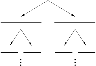
Figure 2: Fragmentation of the support of the probability distribution during the first two steps of the shrinking random walk when $\lambda<1/2$. After $k$ steps, the support fragments into $2^{k}$ intervals each of length $2\lambda^{k}/(1-\lambda)$.

The evolution of the support of the probability distribution can be determined in a precise way by recasting the geometric random walk into the random map,

$$x^{\prime}=\pm 1+\lambda x,$$ (1)

which describes how the position of a particle changes in a single step. We can see that this map is equivalent to the original random walk process by substituting $x^{\prime}$ for $x$ on the right-hand side of Eq. (1) and iterating. Therefore the map is equivalent to the random sum $x=\sum_{n}^{\infty}\epsilon_{n}\lambda^{n}$.

Similarly, the equation for the probability distribution at the $N$th step satisfies the recursion relationreif ; weiss

$$P_{\lambda}(x,N)=\frac{1}{2}\Big{[}P_{\lambda}\big{(}\frac{x-1}{\lambda},N-1\big{)}+P_{\lambda}\big{(}\frac{x+1}{\lambda},N-1\big{)}\Big{]}.$$ (2)

Equation (2) states that for a particle to be at $x$ at the $N$th step, the particle must either have been either at $(x+1)/\lambda$ or at $(x-1)/\lambda$ at the previous step; the particle then hops to $x$ with probability 1/2. For any $\lambda<1$, the probability distribution necessarily approaches a fixed limit $P_{\lambda}(x)$ for $N\to\infty$. Consequently, $P_{\lambda}(x)$ remains invariant under the mapping given by Eq. (1) and thus satisfies the invariance condition

$$P_{\lambda}(x)=\frac{1}{2}\Big{[}P_{\lambda}\big{(}\frac{x-1}{\lambda}\big{)}+P_{\lambda}\big{(}\frac{x+1}{\lambda}\big{)}\Big{]}.$$ (3)

Because $P_{\lambda}(x)$ can have a singular appearance, it often is more useful to characterize this distribution by the probability measure $M_{\lambda}(a,b)$ defined by

$$M_{\lambda}(a,b)=\!\int_{a}^{b}\!dx\,P_{\lambda}(x).$$ (4)

The integral in Eq. (4) smooths out singularities in $P_{\lambda}$ itself, and we shall see that it is more amenable to theoretical analysis. The invariance condition of Eq. (3) can be rewritten in terms of this measure as

$$2M_{\lambda}(a,b)=M_{\lambda}\Big{(}\frac{a-1}{\lambda},\frac{b-1}{\lambda}\Big{)}+M_{\lambda}\Big{(}\frac{a+1}{\lambda},\frac{b+1}{\lambda}\Big{)}.$$ (5)

Equation (5) can now be used to determine the support of $M_{\lambda}$. Clearly, the support of $M_{\lambda}$ lies within the interval $J_{\lambda}=[-x_{\max},x_{\max}]$, with $x_{\max}=1/(1-\lambda)$. For $\lambda<1/2$, the map (1) transforms the interval $J_{\lambda}$ into the union of the two non-overlapping subintervals (see Fig. 2),

$$\Big{[}-\frac{1}{(1-\lambda)},-\frac{(1-2\lambda)}{(1-\lambda)}\Big{]},\ \Big{[}\frac{(1-2\lambda)}{(1-\lambda)},\frac{1}{(1-\lambda)}\Big{]}.$$ (6)

By restricting the map (1) to these two subintervals, we find that they are transformed into four non-overlapping subintervals after another iteration. If we continue these iterations ad infinitum, we obtain a support for $M_{\lambda}$ that consists of a collection of disjoint sets that ultimately comprise a Cantor set.W

On the other hand, for $\lambda\geq 1/2$, the map again transforms $J_{\lambda}$ into the two subintervals given in Eq. (6), but now these subintervals are overlapping. Thus the support of $P_{\lambda}$ fills the entire range $[-x_{\max},x_{\max}]$.

IV Exact Distribution for $\lambda=2^{-1/m}$

In this section, we derive $P_{\lambda}$ by Fourier transform methods for $\lambda=2^{-1/m}$. We will illustrate that the different values of $m$ turn out to be exactly soluble because of a set of fortuitous cancellations in the product form for the Fourier transform of the probability distribution.

For a general random walk process, the probability $P(x,N)$ that the endpoint of the walk is at $x$ at the $(N+1)$ step obeys the fundamental convolution equationreif ; weiss

$$P(x,N)=\sum_{x^{\prime}}P(x-x^{\prime},N-1)\,p_{N}(x^{\prime}),$$ (7)

where $p_{N}(x)$ is the probability of hopping a distance $x$ at the $N^{\rm th}$ step. Equation (7) expresses the fact that to reach $x$ after $(N+1)$ steps the walk must first reach a neighboring point $x-x^{\prime}$ after $N$ steps and then hop from $x-x^{\prime}$ to $x$ at step $(N+1)$. The convolution structure of Eq. (7) cries out for employing Fourier transforms. Thus we introduce

$$p_{N}(k) = \!\int_{-\infty}^{\infty}\!p_{N}(x)\,e^{ikx}\,dx$$

$$P(k,N) = \!\int_{-\infty}^{\infty}\!P(x,N)\,e^{ikx}\,dx,$$ (8)

and substitute these forms into Eq. (7). If the random walk is restricted to integer-valued lattice points, these integrals become discrete sums. The Fourier transform turns the convolution in $x$ into a product in $k$-space,arfken and therefore Eq. (7) becomes the recursion relation

$$P(k,N)=P(k,N-1)\,p_{N}(k).$$ (9)

We now iterate Eq. (9) to obtain the formal solution

$$P(k,N)=P(k,0)\,\prod_{n=0}^{N}p_{n}(k).$$ (10)

Generally, we consider the situation where the random walk begins at the origin. Thus $P(x,0)=\delta_{x,0}$ and correspondingly from the second of Eq. (IV), $P(k,0)=1$. To calculate $P(x,N)$, we evaluate the product in Eq. (10) and then invert the Fourier transform.reif To simplify the notation for the examples of this section, we define $\Pi_{m}(x)=P_{2^{-1/m}}(x)$. We explicitly consider the cases $m=1$, 2, and 3. From these results, the qualitative behavior for general $m$ is then easy to understand.

The single-step probability distribution at the $n$th step is

$$p_{n}(x)=\frac{1}{2}[\delta(x-\lambda^{n})+\delta(x+\lambda^{n})],$$

and the corresponding Fourier transform is

$$p_{n}(k) = \!\int_{-\infty}^{\infty}p_{n}(x)e^{ikx}\,dx=\cos(k\lambda^{n}).$$ (11)

The Fourier transform of the probability distribution after $N+1$ steps is the product of the Fourier transforms of the single-step probabilities.reif ; weiss Thus from Eqs. (10) and (11) we have

$$P_{\lambda}(k,N)=\prod_{n=0}^{N}\cos(k\lambda^{n}).$$ (12)

We now apply this exact solution to the illustrative cases of $\lambda=2^{1/m}$. For the simplest case of $\lambda=2^{-1}$, the step length systematically decreases by a factor of 2. By enumerating all walks of a small number of steps, it is easy to see that the probability distribution is uniformly distributed on a periodic lattice whose spacing shrinks by a factor of two at each step. This is a precursor of the uniform nature of $\Pi_{1}(x)$ in the $N\to\infty$ limit. Algebraically, the product in Eq. (12) can be simplified by using the trigonometric half-angle formula to yield

$$\Pi_{1}(k,N) = \cos k\,\,\cos(k/2)\,\ldots\,\cos(k/2^{N})$$ (13)

$$= \frac{\sin(2k)}{2\sin k}\,\,\frac{\sin k}{2\sin(k/2)}\ldots\frac{\sin(k/2^{N-1})}{2\sin(k/2^{N})}$$

$$= \frac{\sin(2k)}{2^{N+1}\sin(k/2^{N})}$$

$$\to \frac{\sin(2k)}{2k}\ \mbox{as}\ N\to\infty.$$

Thus the inverse Fourier transform gives an amazingly simple result. The probability distribution is merely a square-wave pulse, with $\Pi_{1}=1/4$ on the interval $[-2,2]$ and $\Pi_{1}=0$ otherwise.

The distribution for $\lambda=2^{-1/2}$ can be calculated similarly. The successive cancellation of adjacent numerators and denominators as in Eq. (13) still occurs. These cancellations become more apparent by separating the factors that involve $\sin(k/2^{j})$ and $\sin(k/2^{j+1/2})$. Then by following exactly the same steps as those leading to Eq. (13), we obtain the Fourier transform

$$\Pi_{2}(k)=\frac{\sin(2k)}{2k}\frac{\sin(\sqrt{2}k)}{\sqrt{2}k}.$$ (14)

This product form has a simple interpretation in real space. If we partition the walk into odd steps $(1,3,5,\ldots)$ and even steps $(2,4,6,\ldots)$, then both the odd and even steps are separately geometrical random walks with $\lambda=2^{-1}$, but with the initial step length of the odd walk equal to $1$ and that of the even walk equal to $1/\sqrt{2}$. In real space, the full probability distribution for $\lambda=2^{-1/2}$ is just the convolutions of the constituent distributions for these odd and even walks. Thus in Fourier space, the full distribution is just the product of the constituent distributions, as given in Eq. (14).

Figure 3: Probability distributions for the GW for $\lambda=2^{-1/m}$ for $m=1$, 2, and 3 (dotted, dashed, and solid, respectively).

To invert the Fourier transform in Eq. (14) by a direct approach is straightforward but unwieldy, and the details are given in Appendix A. Another approach is to use the fact that the probability distribution is the convolution of two rectangular-shaped distributions – one in the range $[-2,2]$ for the odd-step walks and the other in $[-\sqrt{2},\sqrt{2}]$ for the even-step walks. Thus

$$\Pi_{2}(x)=\!\int_{-\infty}^{\infty}\!dx^{\prime}\,\Pi_{1}(x^{\prime})\times\sqrt{2}\Pi_{1}\Big{(}\frac{x-x^{\prime}}{\sqrt{2}}\Big{)}.$$ (15)

Either by this direct approach or by straightforward Fourier inversion as given in the Appendix, the final result is (Fig. 3)

$$\Pi_{2}(x)=\begin{cases}\frac{1}{4}&\text{($|x|<2-\sqrt{2}$)}\\ \frac{1}{4}\big{(}1-\frac{|x|}{{2+\sqrt{2}}}\big{)}&\text{$(2-\sqrt{2}<|x|<2+\sqrt{2})$}\\ 0&\text{$(|x|>2+\sqrt{2})$}\end{cases}$$ (16)

Thus the distribution is continuous, but its first derivative is discontinuous at the four points $x=\pm 2\pm\sqrt{2}$.

Continuing this same train of logic, the solution for general $\lambda=2^{-1/m}$ is

$$\Pi_{m}(k)=\frac{\prod_{j=1}^{m}\sin(2^{j/m}k)}{2^{(m+1)/2}k^{m}}.$$ (17)

For example, for $\lambda=2^{-1/3}$, the resulting probability distribution in real space is

$$\Pi_{3}(x)=\begin{cases}\frac{1}{64}(x_{4}^{2}-x_{3}^{2}-x_{2}^{2}-x_{1}^{2}-x^{2})&(|x|<x_{1})\\ \frac{1}{64}(x_{4}^{2}-x_{3}^{2}-x_{2}^{2}-x^{2}-2xx_{1})&(x_{1}<|x|<x_{2})\\ \frac{1}{64}(x_{4}^{2}-x_{3}^{2}-2x(x_{1}+x_{2}))&(x_{2}<|x|<x_{3})\\ \frac{1}{64}(x-x_{4})^{2}&(x_{3}<|x|<x_{4})\\ 0&(|x|>x_{4})\end{cases}$$

where

$$x_{1} = -2+2^{2/3}+2^{1/3}\approx 0.08473$$

$$x_{2} = +2-2^{2/3}+2^{1/3}\approx 1.6725$$

$$x_{3} = +2+2^{2/3}-2^{1/3}\approx 2.3275$$

$$x_{4} = +2+2^{2/3}+2^{1/3}\approx 4.8473$$

This distribution contains both linear and quadratic segments such that the first two derivatives of $\Pi_{3}$ are continuous, but the second derivative is discontinuous at the joining points $x_{j}$, for $j=1$, 2, 3, 4 (Fig. 3). Generally, for $\lambda=2^{-1/m}$, the distribution has continuous derivatives up to order $m-1$, while the $m$th derivative is discontinuous at $2m$ points. As $m\to\infty$, the distribution progressively becomes smoother and ultimately approaches the Gaussian of the nearest-neighbor random walk.

A final note about the Fourier transform method is that it provides a convenient way to calculate the moments,

$$\langle x^{2k}\rangle=\!\int x^{2k}P_{\lambda}(x)\,dx,$$ (19)

for all values of $\lambda$.vanK By expanding $P_{\lambda}(k)$ is a power series for small $k$, we have

$$P_{\lambda}(k) = \!\int\!dx\,P_{\lambda}(x)\,e^{ikx}$$ (20)

$$= \!\int\!dx\,P_{\lambda}(x)\,(1+ikx-k^{2}x^{2}/2!+\ldots)$$

$$= 1-\frac{k^{2}\langle x^{2}\rangle}{2!}+\frac{k^{4}\langle x^{4}\rangle}{4!}+\ldots.$$

That is, the Fourier transform contains all the moments of the distribution. For this reason, the Fourier transform is often termed the moment generating function.

We take the Fourier transform of the probability distribution of the geometric random walk and expand this expression in a power series in $k$ to give

$$P_{\lambda}(k) = \cos k\,\cos(\lambda k)\,\cos(\lambda^{2}k)\ldots$$

$$= \big{[}1\!-\!\frac{k^{2}}{2!}\!+\!\ldots\big{]}\big{[}1\!-\!\frac{(\lambda k)^{2}}{2!}\!+\!\ldots\big{]}\big{[}1\!-\!\frac{(\lambda^{2}k)^{2}}{2!}\!+\!\ldots\big{]}\!\ldots\!$$

$$= 1-\frac{k^{2}}{2}(1+\lambda^{2}+\lambda^{4}+\ldots)+{\cal O}(k^{4}).$$

If we equate the two power series (20) and (IV) term by term, we obtain

$$\langle{x^{2}}\rangle = \frac{1}{1-\lambda^{2}}$$ (21a)

$$\langle{x^{4}}\rangle = \frac{1}{1-\lambda^{4}}\Big{(}1+\frac{6\lambda^{2}}{1-\lambda^{2}}\Big{)}.$$ (21b)

Moments of any order can be obtained by this approach.

V Golden walk

Particularly beautiful behavior of $P_{\lambda}(x)$ occurs when $\lambda=g$ (see Fig. 1(d)). Unfortunately, a straightforward simulation of the geometric random walk is not a practical way to visualize fine-scale details of this probability distribution accurately because the resolution is necessarily limited by the width of the bin used to store the distribution. We now describe an enumeration approach that is exact up to the number of steps in the walk.

V.1 Enumeration

It is simple to specify all walks of a given number of steps. Each walk can be represented as a string of binary digits with 0 representing a step to the left and 1 representing a step to the right. Thus we merely need to list all possible binary numbers with a given number of digits $N$ to enumerate all $N$-step walks. However, we need a method that provides the endpoint location without any loss of accuracy to resolve the fine details of the probability distribution.

Figure 4: First 5 steps of the golden walk enumeration tree. Notice that the distance between adjacent endpoints can only be either $2g^{n}$ or $2g^{n-1}$.

The basic problem of determining the endpoint locations may be illustrated by enumerating the first few steps of the walk and representing them as the branches of a tree as shown in Fig. 4. For $\lambda=g$, neighboring branches of the tree may rejoin because of the existence of 3-step walks (one step right followed by two steps left or vice versa) that form closed loops. For large $N$, the accuracy in the position of a walk is necessarily lost by roundoff errors if we attempt to evaluate the sum for the endpoint location, $X_{N}=\sum_{n}^{N}\epsilon_{n}g^{n}$, directly. Thus the recombination of branches in the tree will eventually be missed, leading to fine-scale inaccuracy in the probability distribution.

However, we may take advantage of the algebra of the golden ratio to reduce the $N$th-order polynomial in $X_{N}$ to a first-order polynomial. To this end, we successively use the defining equation $g^{2}=1-g$ to reduce all powers of $g$ to first order. When we apply this reduction to $g^{n}$, we obtain the remarkably simple formula $g^{n}=(-1)^{n}(F_{n-1}-gF_{n})$, where $F_{n}$ is the $n$th Fibonacci number (defined by $F_{n}=F_{n-1}+F_{n-2}$ for $n>2$, with $F_{1}=F_{2}=1$). For the golden walk, we now use this construction to reduce the location of each endpoint, which is of the form $\sum_{n}^{N}\epsilon_{n}g^{n}$, to the much simpler form $A+Bg$, where $A$ and $B$ are integers whose values depend on the walk. By this approach, each endpoint location is obtained with perfect accuracy. The resulting distribution, based on enumerating the exact probability distribution for $N\leq 29$, is shown in Fig. 5 at various spatial resolutions. At $N=29$ this distribution is exact to a resolution of $10^{-7}$.

V.2 Self-Similarity

Perhaps the most striking feature of the endpoint distribution is its self-similarity, as sketched in Fig. 6. Notice, for example, that the portion of the distribution within the zeroth subinterval $J^{0}=[-g,g]$ is a microcosm of the complete distribution in the entire interval $J=[-g^{-2},g^{-2}]$. In fact, we shall see that the distribution within $J^{0}$ reproduces the full distribution after rescaling the length by a factor $g^{-3}$ and the probability by a factor of 3. Similarly, the distribution in the first subinterval $J^{1}=[g,1+g^{2}]$ reproduces the full distribution after translation to the left by 1, rescaling the length by $g^{-4}$, and rescaling the probability by 6. A similar construction applies for general subintervals.

To develop this self-similarity, it is instructive to construct the symmetries of the probability distribution. Obviously, $P_{g}(x)$ is an even function of $x$. That is,

$$P_{g}(x)=P_{g}(-x).$$ (22)

In fact, there is an infinite sequence of higher-order symmetries that arise from the evenness of $P_{g}(x)$ about the endpoints after 1 step, 2 steps, 3 steps, etc.

For example, the first higher-order symmetry is

$$P_{g}(1+x)=P_{g}(1-x)$$ (23)

for $|x|<g^{2}$. Equation (23) expresses the symmetry of $P_{g}(x)$ about $x=1$ for the subset of walks whose first step is to the right. We can ignore walks whose first step is to the left because the rightmost position of such walks is $-1+g+g^{2}+\ldots=g=1-g^{2}$. Thus within a distance of $g^{2}$ from $x=1$, only walks with the first step to the right contribute to the distribution within this restricted range. The probability distribution must therefore be symmetric about $x=1$ within this same range.

Figure 5: Probability distribution of the golden walk for a 29-step enumeration at spatial resolution $10^{-2}$, $10^{-3}$ and $10^{-4}$ (a) – (c), respectively. In (c), the line joining successive points is not shown so that details of the distribution remain visible.

Continuing this construction, there are infinitely many symmetries of the form

$$P_{g}\big{(}\sum_{n=0}^{k}g^{n}+x\big{)}=P_{g}\big{(}\sum_{n=0}^{k}g^{n}-x\big{)},$$ (24)

with $k=1,2,\ldots$ that represent reflection symmetry about the point that is reached when the first $k$ steps are all in one direction. The $k$th symmetry applies within the range $|x|<g^{k+1}$.

We now exploit these symmetries to obtain a simple picture for the measure of the probability distribution, $M_{g}$. We start by decomposing the full support $J$ into the contiguous subintervals that span the successive lobes of the distribution, as shown in Fig. 6. We label these subintervals as $J^{0}=(-g,g)$, $J^{1}=(1-g^{2},1+g^{2})$, $J^{2}=(1+g-g^{3},1+g+g^{3})$, etc.; there are also mirror image intervals to the left of the origin, $J^{-k}=-J^{k}$.

We now use the invariance condition of Eq. (5) to determine the measures of these fundamental intervals $J^{k}$. For $J^{0}=(-g,g)$, this invariance condition yields

$$M_{g}(-g,g) = \frac{1}{2}[M_{g}(-(2+g),-g)+M_{g}(g,2+g)]$$ (25)

$$= \frac{1}{2}[1-M_{g}(-g,g)],$$

where the second line follows because of left-right symmetry and because the intervals $(-(2+g),-g)$, $(g,2+g)$, and $(-g,g)$ comprise the entire support of a normalized distribution. We therefore obtain the remarkably simple result that the measure of the central interval is $M_{g}(-g,g)=1/3$. If we apply the same invariance condition to $J^{1}$, we find $M_{g}(J^{1})=\frac{1}{2}M_{g}(J^{0})$. By continuing this same reasoning to higher-order intervals $J^{K}$, we find, in general, that the measure of the $k$th interval is one-half that of the previous interval (see Fig. 6). Thus we obtain the striking result

$$M_{g}(J^{k})=\frac{1}{3\cdot 2^{|k|}}.$$ (26)

Figure 6: Sketch to illustrate the symmetry and self-similarity of $P_{g}(x)$. The dashed curve is the probability distribution when the first step is to the right. The full probability distribution is the sum of the dashed curve and an identical (but shifted) curve that stems from the distribution when the first step is to the left. The measures associated with each lobe of $P_{\lambda}(x)$ (top) and the spatial extent of each lobe (bottom) are indicated. Notice that the left extreme of the restricted distribution coincides with the first minimum of the full distribution.

V.3 Singularities

Another intriguing feature of $P_{g}(x)$ is the existence of a series of deep minima in the distribution. Consider, for example, the most prominent minima at $x=\pm g$ (see Fig. 5). The mechanism for these minima is essentially the same reason that $g$ is sometimes termed the “most irrational” real number – that is, most difficult to approximate by a rational number.numbers In fact, there is only a single trajectory of the random walk in which the endpoint of the walk reaches $g$, namely, the trajectory that consists of alternating the steps, $1-g+g^{2}-g^{3}+g^{4}-\ldots$. If there is any deviation from this alternating pattern, the endpoint of the walk will necessarily be a finite distance away from $x=g$. This dearth of trajectories with endpoints close to $x=g$ is responsible for the sharp minimum in the probability distribution.

More generally, this same mechanism underlies each of the minima in the distribution, including the singularity as $x\to x_{\max}$. For each local minimum in the distribution, the first $n$ steps of the walk must be prescribed for the endpoint to be within a distance of the order of $g^{n}$ to the singularity. However, specifying the first $n$ steps means that the probability for such walks can be no greater than $2^{-n}$. It is this reduction factor that leads to all the minima in the distribution.

For simplicity, we focus on the extreme point in the following; the argument for all the singularities is similar. If the first $n$ steps are to the right, then the maximum distance $\Delta$ between the endpoint of the walk and $x_{\max}$ arises if the remaining steps are all to the left. Therefore

$$\Delta=x_{\max}-(1+g+\ldots+g^{n})+g^{n+1}+g^{n+2}+\ldots=2g^{n-1}.$$

Correspondingly, the total probability to have a random walk whose endpoint is within this range is simply $2^{-n}$.

For $x$ near $x_{\max}$, we make the fundamental assumption that $P_{\lambda}(x)\sim(x_{\max}-x)^{\mu}$. Although this hypothesis appears difficult to justify rigorously for general values of $\lambda$, such a power law behavior arises for $\lambda=2^{-1/m}$, as discussed in Sec. III. We assume that power-law behavior continues to hold for general $\lambda$ values. With this assumption, the measure for a random walk to be within the range $\Delta=x_{\max}-x$ of $x_{\max}$ is $M(\Delta)\sim\Delta^{1+\mu}$. However, because such walks have the first $n$ steps to the right, $M(\Delta)$ also equals $2^{-n}$. If we write $\ln M=-n\ln 2$, $\ln\Delta=+(n-1)\ln g+\ln 2$, and eliminate $n$ from these relations, we obtain $M(\Delta)\sim\Delta^{\ln 2/\ln(1/g)}$ or, finally,

$$P_{g}(\Delta)\sim\Delta^{-1+\ln 2/\ln(1/g)}.$$ (27)

This power law also occurs at each of the singular points of the distribution because the underlying mechanism is the same as that for the extreme points.

The same reasoning applies mutatis mutandis near the extreme points for general $\lambda$, leading to the asymptotic behavior $P_{\lambda}(\Delta)\sim\Delta^{-1+\ln 2/\ln(1/\lambda)}$. In particular, this reason gives, for the tail of $\Pi_{m}$, the limiting behavior $\Delta^{m-1}$, in agreement with the exact calculation in Sec. III.

VI Discussion

We have outlined a number of appealing properties of random walks with geometrically shrinking steps, in which the length of the $n$th step equals $\lambda^{n}$ with $\lambda<1$. A very striking feature is that the probability distribution of this walk depends sensitively on the shrinkage factor $\lambda$ and much effort has been devoted to quantifying the probability distribution. We worked out the probability distribution for the special cases $\lambda=2^{-1/m}$ where a solution is possible by elementary means. We also highlighted the beautiful self-similarity of the probability distribution when $\lambda=(\sqrt{5}-1)/2$. Here, the unique features of this number facilitate a numerically exact enumeration method and also lead to very simple results for the probability measure.

We close with some suggestions for future work. What is the effect of a bias on the limiting probability distribution of the walk? For example, suppose that steps to the left and right occur independently and with probabilities $p$ and $1-p$ respectively. It has been provenPS98 that the probability distribution is singular for $\lambda<p^{p}(1-p)^{1-p}$ and is continuous for almost all larger values of $\lambda$. This is the analog of the transition at $\lambda=1/2$ for the isotropic case. What other mysteries lurk within the anisotropic system?

Are there interesting first-passage characteristics? For example, what is the probability that a walk, whose first step is to the right, never enters the region $x<0$ by the $n$th step? Such questions are of fundamental importance in the classical theory of random walks,weiss and it may prove fruitful to extend these considerations to geometric walks. Clearly, for $\lambda<1$, this survival probability will approach a non-zero value as the number of steps $N\to\infty$. How does the survival probability converge to this limiting behavior as a function of the number of steps? Are there qualitative changes in behavior as $\lambda$ is varied?

What happens in higher spatial dimensions? This extension was suggested to us by M. Bazant.bazant1 There are two natural alternatives that appear to be unexplored. One natural way to construct the geometric random walk in higher dimensions is to allow the direction of each step to be isotropically distributed, but with the length of the $n$th step again equal to $\lambda^{n}$. Clearly, if $\lambda\ll 1$, the probability distribution is concentrated within a spherical shell of radius 1 and thickness of the order of $\lambda/(1-\lambda)$. As $\lambda$ is increased, the probability distribution eventually develops a peak near the origin.bazant What is the nature of this qualitative change in the probability distribution? Another possibilitybrad is to require that the steps are always aligned along the coordinate axes. Then for sufficiently small $\lambda$ the support of the walk would consist of a disconnected set, while as $\lambda$ increases beyond 1/2, a sequence of transitions similar to those found in one dimension may arise.

Appendix A Fourier Inversion of the Probability Distribution for $\lambda=2^{-1/2}$

For $\lambda=2^{-1/2}$, we write $P_{\lambda}(k)$ in the form

$$\Pi_{2}(k) = \frac{\sin(2k)\sin(\sqrt{2}k)}{2^{3/2}k^{2}}$$ (28)

$$= -\frac{(e^{2ik}-e^{-2ik})(e^{\sqrt{2}ik}-e^{-\sqrt{2}2ik})}{2^{7/2}k^{2}}$$

$$\equiv -\frac{[e^{ikx_{2}}+e^{-ikx_{2}}-e^{ikx_{1}}-e^{-ikx_{1}}]}{{2^{7/2}k^{2}}},$$

where $x_{1}=2-\sqrt{2}$ and $x_{2}=2+\sqrt{2}$. The inverse Fourier transform is

$$\Pi_{2}(x)=\frac{1}{2\pi}\!\int_{-\infty}^{\infty}\!\Pi_{2}(k)\,e^{-ikx}\,dk.$$ (29)

To evaluate the integral, we extend it into the complex plane by including a semi-circle at infinity. The outcome of this inverse transform depends on the relation between $x$ and $x_{1}$, $x_{2}$.

For $x>x_{2}$, we must close the contour in the lower half-plane for each term, so that the semi-circle contribution is zero. We must also indent the contour around an infinitesimal semi-circle about the origin to avoid the singularity at $k=0$. If $x>x_{2}$, the residues associated with each term in the integrand cancel, and we obtain $\Pi_{2}(x)=0$.

For $0<x<x_{1}$, we must close the contours in the upper half-plane for the first and third terms, and in the lower-half plane for the complementary terms. The contribution of the first integral is proportional to

$$\oint\frac{e^{ik(x_{2}-x)}}{k^{2}}\,dk=i\pi\mbox{Res}\Big{[}\frac{e^{ik(x_{2}-x)}}{k^{2}}\Big{]}\Bigg{|}_{k=0}=-\pi(x_{2}-x).$$

Similarly, the contributions of the remaining three integrals are $-\pi(x_{2}+x)$, $-\pi(x_{1}-x)$,and $-\pi(x_{1}+x)$, respectively. As a result, we find, for $0<x<x_{1}$,

$$\Pi_{2}(x)=\frac{(x_{2}-x)+(x_{2}+x)-(x_{1}-x)-(x_{1}+x)}{2^{9/2}}=\frac{1}{4}.$$

Finally, for $x_{1}<x<x_{2}$, we must close the contour in the upper half-plane for the first two terms in Eq. (29) and in the lower-half plane for the latter two terms. Evaluating each of the residues, we now obtain, for $x_{1}<x<x_{2}$

$$\Pi_{2}(x)=\frac{1}{4}\big{(}1-\frac{x}{x_{2}}\big{)}.$$

References

- (1) B. Jessen and A. Wintner, “Distribution functions and the Riemann zeta function”, Trans. Amer. Math. Soc. 38, 48-88 (1935); B. Kershner and A. Wintner, “On symmetric Bernoulli convolutions”, Amer. J. Math. 57, 541-548 (1935); A. Wintner, “On convergent Poisson convolutions”, ibid. 57, 827-838 (1935).
- (2) P. Erdős, “On a family of symmetric Bernoulli convolutions”, Amer. J. Math. 61, 974-976 (1939); P. Erdős, “On smoothness properties of a family of Bernoulli convolutions”, ibid. 62, 180-186 (1940).
- (3) A. M. Garsia, “Arithmetic properties of Bernoulli convolutions”, Trans. Amer. Math. Soc. 102, 409-432 (1962); A. M. Garsia, “Entropy and singularity of infinite convolutions”, Pacific J. Math. 13, 1159-1169 (1963).
- (4) M. Kac, Statistical Independence in Probability, Analysis and Number Theory (Mathematical Association of America; distributed by Wiley, New York, 1959).
- (5) E. Barkai and R. Silbey, “Distribution of single-molecule line widths”, Chem. Phys. Lett. 310, 287-295 (1999).
- (6) E. Ben-Naim, S. Redner, and D. ben-Avraham, “Bimodal diffusion in power-law shear flows,” Phys. Rev. A 45, 7207-7213 (1992).
- (7) J. C. Alexander and J. A. Yorke, “Fat baker’s transformations”, Ergodic Th. Dynam. Syst. 4, 1-23 (1984); J. C. Alexander and D. Zagier, “The entropy of a certain infinitely convolved Bernoulli measure”, J. London Math. Soc. 44, 121-134 (1991).
- (8) F. Ledrappier, “On the dimension of some graphs”, Contemp. Math. 135, 285-293 (1992).
- (9) Y. Peres, W. Schlag, and B. Solomyak, “Sixty years of Bernoulli convolutions”, in Fractals and Stochastics II, edited by C. Bandt, S. Graf, and M. Zähle (Progress in Probability, Birkhauser, 2000), Vol. 46, pp. 39-65.
- (10) P. Diaconis and D. Freedman, “Iterated Random Functions”, SIAM Rev. 41, 45-76 (1999).
- (11) A. C. de la Torre, A. Maltz, H. O. Mártin, P. Catuogno, and I. Garciá-Mata, Phys. Rev. E 62, 7748-7754 (2000).
- (12) F. Reif, Fundamentals of Statistical and Thermal Physics (McGraw Hill, New York, 1965).
- (13) G. H. Weiss, Aspects and Applications of the Random Walk (North-Holland, Amsterdam 1994); S. Redner, A Guide to First-Passage Processes (Cambridge University Press, New York, 2001).
- (14) See, for example, lecture notes by M. Bazant for MIT course 18.366. The URL is <http://www-math.mit.edu/18.366/>.
- (15) B. Solomyak, “On the random series (an Erdős problem)”, Ann. Math. 142, 611-625 (1995).
- (16) M. J. Bertin, A. Decomps-Guilloux, M. Grandet-Hugot, M. Pathiaux-Delefosse, Pisot and Salem numbers (Birkhäuser, Boston, 1992).
- (17) F. Ledrappier and A. Porzio, “A dimension formula for Bernoulli convolutions”, J. Stat. Phys. 76, 1307-1327 (1994).
- (18) N. Sidorov and A. Vershik, “Ergodic properties of Erd s measure, the entropy of the goldenshift, and related problems”, Monatsh. Math. 126, 215-261 (1998).
- (19) G. B. Arfken, Mathematical Methods for Physicists (Academic Press, San Diego, 1995).
- (20) See for example, N. G. van Kampen, Stochastic Processes in Physics and Chemistry (North-Holland, Amsterdam, 1992).
- (21) J. H. Conway and R. K. Guy, The Book of Numbers (Springer, New York, 1996).
- (22) Y. Peres and B. Solomyak, “Self-similar measures and intersections of Cantor sets”, Trans. Am. Math. Soc. 350, 4065-4087 (1998).
- (23) M. Bazant, B. Bradley, and J. Choi, unpublished.
- (24) B. Bradley, private communication.